Research Collection
Journal Article
High-resolution high-speed void fraction measurements in helically coiled tubes using X-ray radiography
Author(s):
Breitenmoser, David; Manera, Annalisa; Prasser, Horst-Michael; Adams, Robert; Petrov, Victor Publication Date:
2021-05
Permanent Link:
https://doi.org/10.3929/ethz-b-000467071
Originally published in:
Nuclear Engineering and Design 373, http://doi.org/10.1016/j.nucengdes.2020.110888
Rights / License:
Creative Commons Attribution-NonCommercial-NoDerivatives 4.0 International
This page was generated automatically upon download from the ETH Zurich Research Collection. For more
information please consult the Terms of use.
Nuclear Engineering and Design 373 (2021) 110888
Available online 26 January 2021
0029-5493/© 2020 The Authors. Published by Elsevier B.V. This is an open access article under the CC BY-NC-ND license
(http://creativecommons.org/licenses/by-nc-nd/4.0/).
High-resolution high-speed void fraction measurements in helically coiled tubes using X-ray radiography
David Breitenmoser
a,b,*, Annalisa Manera
a, Horst-Michael Prasser
b, Robert Adams
b, Victor Petrov
aaExperimental and Computational Multiphase Flow Laboratory, Department of Nuclear Engineering and Radiological Sciences, University of Michigan, 2355 Bonisteel Blvd, Ann Arbor, MI 48109-2104, USA
bLaboratory of Nuclear Energy Systems, Institute of Energy Technology, Department of Mechanical and Process Engineering, Swiss Federal Institute of Technology, Sonneggstrasse 3, Zurich, 8092, Switzerland
A R T I C L E I N F O Keywords:
Flow regime Helically coiled tube Two-phase flow Void fraction X-ray radiography
A B S T R A C T
Helical coil heat exchangers are known for their superior heat transfer, compactness and robustness against thermal expansion compared to systems with straight pipes. Due to all these benefits, they became quite popular in the last few decades in various industries such as pharmaceutical, chemical or nuclear. Generally, they are used in a single-phase environment or with evaporation taking place on the shell side. However, in most of the steam generator designs adopted in advanced nuclear reactors, the two-phase mixture flows upward within the vertically oriented helical coils. In addition, physical two-phase phenomena taking place inside helical tubes differ significantly from those in straight pipes due to inherent centrifugal and torsion effects. To improve the computational models used to predict the thermal hydraulic performance of such steam generators, experimental characterization and identification of different two-phase flow patterns in helical coils are essential. In the present paper, high-resolution measurements of the void fraction distribution for an adiabatic upward air–water two-phase flow were conducted in a transparent helically coiled acrylic pipe by means of high-speed X-ray radiography at ambient conditions. Various void fraction based features such as probability density function estimates, profiles over the height of the pipe cross-section and temporal evolutions were used to identify and characterize flow regimes. A total of 13 measurements are presented in this paper, classified into six flow re- gimes, namely: bubbly, plug, wavy, slug, slug-annular and annular flow. The obtained flow regimes are in accordance with flow regime characterizations and transition criteria already reported in literature.
1. Introduction
Helically coiled tubes or helical coils for short are often used today as basic heat transfer elements in boilers, evaporators or refrigerating systems due to their excellent heat transfer performance, compactness and robustness against thermal stresses (Zhu et al., 2017). In the nuclear engineering field, helically coiled steam generators are part of a variety of innovative Generation-IV nuclear power plant designs such as the sodium-cooled fast reactors (SFR) (Chetaland and Vaidyanathan, 1997), the lead-cooled fast reactors (LFR) (Dragunov et al., 2012) or the high- temperature gas cooled reactors (HTGR) (B¨aumer et al., 1990; Quade et al., 1974; Wu et al., 2002; Zhang et al., 2016). Especially since this type of steam generators can be designed and built very compactly, they are also considered for advanced small modular reactors (SMR), e.g. the
International Reactor Innovative Secure (IRIS) project (Carelli et al., 2004), the System-Integrated Modular Advanced Reactor (SMART) (Kim et al., 2013), the CAREM-25 reactor (Marcel et al., 2013) or the NuScale power module (Ingersoll et al., 2014), among others.
The thermal hydraulic performance of helically coiled steam gener- ators differs significantly from those of commercial nuclear reactors. In contrast to most of the Generation-II and Generation-III reactors, the evaporating working fluid of the turbine circuit, i.e. a gas–liquid two- phase mixture, is forced upward through the vertically oriented coils whereas the primary coolant flows downward at the shell side (Kim et al., 2013). Depending on the operational conditions, different inter- facial topologies may develop within the helical coils. The identification and prediction of these flow patterns or flow regimes are of great importance for the design and operation of helically coiled steam gen- erators since all fundamental thermal hydraulic processes such as heat,
* Corresponding author.
E-mail address: david.breitenmoser@alumni.ethz.ch (D. Breitenmoser).
Contents lists available at ScienceDirect
Nuclear Engineering and Design
journal homepage: www.elsevier.com/locate/nucengdes
https://doi.org/10.1016/j.nucengdes.2020.110888
Received 19 March 2020; Received in revised form 9 September 2020; Accepted 2 October 2020
mass and momentum transfer are intrinsically linked to the established flow regimes. In the past 50 years, the majority of the studies examining flow regimes focused on straight pipes (Cheng et al., 2008). There is still some controversy in the pertinent literature regarding the impact of the helical coil geometrical configuration on the frictional pressure drop for two phase flows (Fsadni et al., 2016). Nevertheless, various experi- mental studies have shown that the heat and mass transfer are signifi- cantly enhanced for helically coiled tubes compared to straight pipes due to inherent centrifugal and torsion forces (Fsadni and Whitty, 2016;
Hameed and Muhammed, 2003). Therefore, thermal hydraulic correla- tions developed for straight pipes have very limited use and become impractical for coils with high curvature and pitch. To improve the predictive capabilities of two-phase flow models for helical coils, it is essential to have accurate experimental data of the void fraction dis- tribution in helical coil geometries.
So far, only a limited amount of experimental studies was performed to investigate the flow patterns in helical coil configurations relevant for the nuclear application, i.e. an upward gas–liquid two-phase flow within the vertically oriented helically coiled tubes. One of the first experi- mental studies about flow patterns in helical coils was published by Banerjee et al. (1969). They analyzed flow patterns inside helical coils for different curvature ratios and pitches by means of high-speed im- aging, differential pressure and hold-up measurements. Further, they used different fluids for the liquid phase, i.e. water and oil. Slug, wavy, slug-annular and annular flow patterns were observed. Their results indicate a fundamental similarity between flow regimes in horizontal straight tubes and flow regimes in helical coils with small helix angles.
The same conclusion was drawn by Akagawa et al. (1971) based on their experimental study. They analyzed bubbly, plug, slug and slug-annular flow regimes by visual inspection, conductivity probes and hold-up measurements. Whalley (1980) examined the transition between the stratified and annular flow regime. In addition, liquid film thickness and liquid film flowrate measurements were conducted. Chen and Zhou
(1981) investigated air–water two-phase flow patterns in a helical coil with a comparatively small helix angle by visual observations. They detected dispersed bubbly, elongated bubbly, slug, stratified, wavy and annular flow regimes. Kaji et al. (1983) applied also visual observations to examine air–water two-phase flow patterns in helically coiled tubes.
In addition, they measured liquid film thicknesses by needle probes and compared their classified flow measurements with Mandhane’s flow map for horizontal straight pipes (Mandhane et al., 1974) and Barnea’s flow map for inclined straight pipes (Barnea et al., 1980). Two inter- esting conclusions can be drawn from their results. First, no smooth stratified flow was observed. This is in line with observations for in- clined straight pipes (Barnea et al., 1980). Second, the other flow re- gimes are fundamentally similar to those observed for inclined straight tubes. Similar results were obtained by Saxena et al. (1990). Murai et al.
(2005, 2006) investigated air–water two-phase flow patterns in helical coils by means of an innovative high-speed image tomography tech- nique and synchronized differential pressure fluctuation measurements.
They observed three different flow regimes, i.e. bubbly, plug and slug.
The tomographic results revealed a significant distortion of local flow pattern features caused by the centrifugal force. Cui et al. (2008) examined flow patterns for a refrigerant R134a boiling flow in micro- finned helical coils by high-speed imaging and differential pressure measurements. They detected stratified-wavy, intermittent and annular flows. It is worth noting that Cui et al. included the bubbly, plug and slug flow in the intermittent flow regime and the annular and slug-annular flow in the annular flow regime. Thandlam et al. (2015) performed an extensive study of flow patterns for different helical coil configurations as well as for Newtonian and non-Newtonian liquids together with air.
They discovered three different flow regimes, i.e. plug, slug and strati- fied flow. An increase of the non-Newtonian liquid concentration induced a significant change of the transitions between the different flow regimes. They explained this by the change of viscosity and consequently a change of the momentum transfer between the phases.
Nomenclature Latin Symbols
D Coil diameter [m]
d Inner tube diameter [m]
E Normalized intensity for air flow [-]
F Normalized intensity for water flow [-]
H Pitch [m]
I Normalization constant [-]
j Superficial velocity [ms−1] k Helical curvature [m−1] L Coil length [m]
Lchord Chord length [m]
L1 Source-to-sample distance [m]
L2 Sample-to-detector distance [m]
N Number of frames [-]
PDF Probability density function [-]
p Two-phase pressure [Pa]
T Temperature [◦C]
TP Normalized intensity for two-phase flow [-]
t Wall thickness [m]
W Void fraction window [-]
Wnorm Normalization window [-]
wchord Chordal weighting factor [-]
x Longitudinal variable y Radial variable Greek Symbols
α Void fraction [-]
β Helix angle [◦]
γ Inclination angle of the beam line [◦] λ Curvature ratio [-]
σ Sample standard deviation [-]
τ Torsion [m−1] Subscripts
a Air
i Radial index j Longitudinal index
k Temporal index
w Water
Acronyms
ADU Analog-to-digital unit
ECMFL Experimental and computational multiphase flow laboratory
FPGA Field programmable gate array HTGR High-temperature gas-cooled reactor
IAPWS International association for the properties of water and steam
IRIS International reactor innovative secure LFR Lead-cooled fast reactor
MAHICan Michigan adiabatic helical coil
NEAMS Nuclear energy advanced modeling and simulation NIST National institute of standards and technology SFR Sodium-cooled fast reactor
SMART System-integrated modular advanced reactor SMR Small modular reactor
So far, all discussed studies used helically coiled pipes with circular cross-sections. Liu et al. (2015) analyzed air–water two-phase flow patterns in rectangular helically coiled channels with a comparatively large helix angle by high-speed imaging and digital image post- processing. Bubbly, intermittent and annular flow patterns were observed. They compared their results with Taitel’s flow map for ver- tical straight tubes (Taitel et al., 1980). Considering the large helix angle, they stated that there are significant similarities between the flow patterns in vertical straight pipes and helical coils with steep in- clinations. Zhu et al. (2017) published one of the most recent papers on flow patterns for air–water two-phase flows in helically coiled pipes.
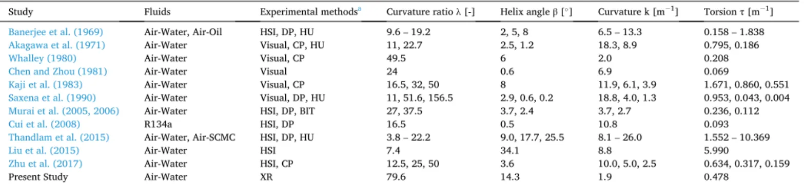
They used high-speed imaging and conductivity needle probes to examine the flow patterns in helical coils for three different configura- tions. With the help of the conductivity needle probes, they measured the bubble chord length, the slug length and the local void fraction. They encountered in total six different flow regimes: bubbly, plug, slug, wavy, slug-annular and annular flow regimes and defined these regimes by linguistic and quantitative descriptions. Zhu et al. provided also new transition criteria based on local time averaged void fractions together with bubble, plug and slug lengths. The detailed helical coil configura- tions together with the applied experimental techniques for the dis- cussed studies are summarized in Table 1. The listed geometrical parameters are discussed in more detail in the following section.
To the best of the authors’ knowledge, flow regime identification in helically coiled tubes has so far only been performed by optical imaging techniques, hold-up measurements by the quick-closing valve method, differential pressure measurements and conductivity probes (cf.
Table 1). Most of the optical methods are entirely qualitative and require optical access to the test section. Global energetic parameters such as differential pressure fluctuations (Matsui, 1984), temperature fluctua- tions (Kozma et al., 1996) or pipe vibrations (Miwa et al., 2015) provide only temporally resolved data, not spatially resolved. In contrast, void fraction based techniques allow reconstruction of some structures of the local two-phase flow topology spatially as well as temporally. In general, there is a variety of techniques for void fraction measurement in two- phase flows, including conductivity probes (Neal and Bankoff, 1963), hot wire anemometers (Toral, 1981), wire-mesh sensors (Prasser et al., 1998), ultrasonic transmission (Xu and Xu, 1997) or radiation attenua- tion based techniques, e.g. gamma-ray densitometry (Abouelwafa and Kendall, 1980) or X-ray radiography (Jones and Zuber, 1975), among others. Radiation based techniques have the advantages that they are non-intrusive as well as non-invasive and that the calibration is simple compared to other methods (Kendoush, 1992).
In the present study, a high-resolution high-speed X-ray radiography system is used to characterize adiabatic upward air–water two-phase flows in a helical coil test section by means of quantitative void frac- tion measurements and to classify each flow measurement into six flow regimes according to the methodology introduced by Zhu et al. (2017), namely: bubbly, plug, wavy, slug, slug-annular and annular flow. X-ray
radiography is a well-established and validated experimental technique to analyze multiphase flows and to extract quantitative volume fraction data of the individual phases (Heindel, 2011). Based on early applica- tions to examine fluidized beds (Grohse, 1955), Pike et al. (1965) pre- sented a standard methodology to analyze two-phase gas–liquid flows by means of X-ray radiography. Using this methodology, Jones and Zuber (1975) as well as Vince and Lahey (1982) proved the suitability of the X-ray radiography technique for classifying flow regimes of gas–liquid flows in simple straight pipe systems.
This study is a continuation of the work performed by Zhuang et al.
(2018). Three main modifications were implemented. First, improved post-processing is applied to the X-ray raw images. Second, the data acquisition system has been modified utilizing the capabilities of Field Programmable Gate Array (FPGA) modules which allow a higher sensor sampling rate. And third, the exposure time per frame of the X-ray system was reduced by a factor of 20, which helped to reduce the motion blurring of the images, and in parallel the frame rate has been increased by 18% while maintaining the same order of contrast-to-noise ratio as in the previous study.
2. Experimental setup
2.1. Air-Water Two-Phase flow loop
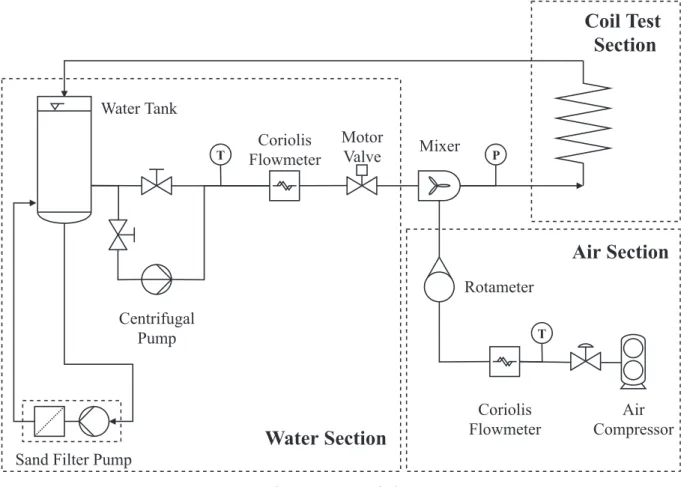
All experiments were performed in the Michigan Adiabatic Helical Coil (MAHICan) test facility, which is located in the Experimental and Computational Multiphase Flow Laboratory (ECMFL) at the University of Michigan. The facility is designed to perform adiabatic upward air–water two-phase flow experiments in helically coiled pipes at ambient conditions and consists of three main sections: the water supply system, the air supply system and the helical coil test section (cf. Fig. 1).
The water supply system consists of a GOULDS GT 203 centrifugal pump controlled by an ABB® 3-phase frequency control drive, a water tank, a thermocouple from McMaster-Carr®, T type, to measure the water temperature and a Coriolis flow meter from Endress +Hauser, Promass 63MT08, to measure the water mass flow rate. A separate filtering loop with a sand filter pump from INTEX®, type 10SF671, cleans the water automatically once a day. On the air side, an in-house air compressor provides ambient air. The air temperature is measured by the same type of thermocouple from McMaster-Carr® as for the water section. A Coriolis flow meter from Endress +Hauser, Promass 83E08, is used to measure the air mass flow rate. The air flow rate is controlled manually by a KING® rotameter, type 7530, with an embedded needle valve. The water and air are mixed in a mixing chamber (cf. Fig. 2). The water is forced through a honeycomb-structured grid whereas the air is injected into the water through a replaceable air sparger. The absolute pressure of this two-phase mixture is measured right after the mixing chamber by means of a pressure gauge Omega PX409-050GI-XL. The air–water two-phase flow is then feed into the helical coil test section.
Table 1
Experimental studies on upward gas–liquid two-phase flow regimes in vertically oriented helically coiled tubes.
Study Fluids Experimental methodsa Curvature ratio λ [-] Helix angle β [◦] Curvature k [m−1] Torsion τ [m−1] Banerjee et al. (1969) Air-Water, Air-Oil HSI, DP, HU 9.6 – 19.2 2, 5, 8 6.5 – 13.3 0.158 – 1.838
Akagawa et al. (1971) Air-Water Visual, CP, HU 11, 22.7 2.5, 1.2 18.3, 8.9 0.795, 0.186
Whalley (1980) Air-Water Visual, CP 49.5 6 2.0 0.208
Chen and Zhou (1981) Air-Water Visual 24 0.6 6.9 0.069
Kaji et al. (1983) Air-Water Visual, CP 16.5, 32, 50 8 11.9, 6.1, 3.9 1.671, 0.860, 0.551
Saxena et al. (1990) Air-Water Visual, DP, HU 11, 51.6, 156.5 2.9, 0.6, 0.2 18.8, 4.0, 1.3 0.953, 0.043, 0.004
Murai et al. (2005, 2006) Air-Water HSI, DP, BIT 27, 37.5 3.7, 2.4 3.7, 2.7 0.236, 0.112
Cui et al. (2008) R134a HSI, DP 16.5 0.5 10.8 0.093
Thandlam et al. (2015) Air-Water, Air-SCMC HSI, DP, HU 3.8 – 22.2 9.0, 17.7, 25.5 8.1 – 26.0 1.552 – 10.369
Liu et al. (2015) Air-Water HSI 7.4 34.1 8.8 5.990
Zhu et al. (2017) Air-Water HSI, CP 12.5, 25, 50 3.6 10.0, 5.0, 2.5 0.634, 0.317, 0.159
Present Study Air-Water XR 79.6 14.3 1.9 0.478
aOnly methods are listed which were involved in the flow pattern analysis. HSI: High-Speed Imaging, CP: Conductivity Probe, BIT: Backlight Image Tomography, DP: Differential Pressure Measurement, HU: Hold-Up measurement with quick-closing valve method, XR: X-Ray Radiography.
After passing through the test section, the two-phase mixture flows back to the water tank, where the air is separated by gravity and released to the environment. The accuracy and range of each measuring instrument used for the experiments is listed in Table 2.
The helically coiled tube, as shown schematically in Fig. 3, is made of transparent cast acrylic with an inner pipe diameter (d) of 12.57 mm, a coil diameter (D) of 1 m and a pitch (H) of 0.8 m. It has a helix angle (β) of 14.3◦ and a curvature ratio (λ) of about 79.6. The dimensionless curvature ratio is defined as the ratio between the coil and the inner tube diameter:
λ=D/d (1)
The helical curvature (k) and torsion (τ) parameters characterize the geometrical contribution to the centrifugal and torsion forces present in the helical coil and can be calculated as follows:
k= 2
D[1+tan2(β)] (2)
Fig. 1. MAHICan test facility.
Fig. 2.Two-phase flow mixing chamber.
Table 2
Measuring instruments.
Instrument Parameter Model Range Accuracy
Coriolis flowmeter Water flow rate Endress +Hauser, Promass 63MT08 0 ~ 30 kg/min ±0.5%
Coriolis flowmeter Air flow rate Endress +Hauser, Promass 83E08 0 ~ 15 kg/min ±0.5%
Pressure transducer Gauge pressure Omega PX409-050GI-XL 0 ~ 100 psi ±1%
Thermocouple Temperature McMaster-Carr®, T type −198 ~ 371 ◦C ±0.75%
Fig. 3. Schematic of the helical coil test section.
τ= 2tan(β)
D[1+tan2(β)] (3)
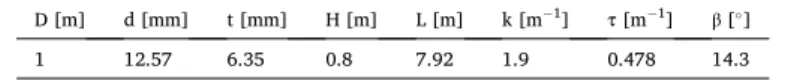
The MAHICan facility is characterized by a helical curvature of 1.9 m−1 and a torsion of 0.478 m−1. All geometrical parameters of the helically coiled pipe used for the experiments are summarized in Table 3. To prevent strong vibrations of the helical coils, the pipes in the helical coil section are mounted with shock-absorbing and vibration- damping clamps. To examine the efficiency of these vibration damp- ing measures, a vibration analysis of the helical coils was performed by means of high-speed imaging. A Phantom Miro LAB 340 (4MP) high- speed camera with a pixel resolution of 1216 ×952 and a frame rate of 2.5 kHz was used. The maximum vibration amplitude obtained from the camera recordings was determined to be 0.1 mm for the range of operational conditions used in the experiments.
2.2. X-Ray radiography
The X-ray radiography system consists of an X-ray tube HF100H with a maximum voltage of 100 kV and a fixed current of 20 mA. The X-ray tube is combined with an image intensifier from Siemens®, model HIDEQ 23–3 ISX, with a fast response phosphor screen and coupled to a high-speed low-noise sCMOS camera PCO.EDGE-5.5. A technical scheme of the setup is shown in Fig. 4. The distances between the X-ray tube and the helical coil (L1) and between the helical coil and the image intensifier (L2) were set to 0.52 ±0.01 m and 0.17 ±0.01 m, respec- tively. The beam axis is inclined by 11.5 ± 0.2◦ (γ). To reduce the exposure time per frame, all experiments were performed at an X-ray tube voltage of 100 kV. A sampling frequency of 68.72 Hz with an exposure time of 0.1 ms was used. The spatial resolution cutoff was determined to be 3.1 lp/mm by means of line pair gauges. The pixel resolution of the camera was set to 1696 ×1351. The X-ray measure- ments were performed 5.42 m downstream of the helical coil pipe entrance, which corresponds to a coil length to inner pipe diameter ratio (L/d) of 431, to minimize entrance effects.
3. Methodology
In this section, the post-processing procedure of the X-ray images and the calculation approach for the void fraction are presented and dis- cussed. The MATLAB® 2019b code was used on a LENOVO® Think- Centre® E73 personal computer, model 10DR001EM2, for all numerical calculations and data processing steps.
3.1. Image post-processing
Before computing the void fraction, the raw images are post- processed in six steps. First, the raw images are filtered by a two- dimensional median filter with a local filter size of 5 by 5 pixel to reduce salt-and-pepper noise. Second, to account for the spatial over- sampling by the X-ray acquisition system, a pixel binning algorithm is applied to the raw images. With a pixel-to-length ratio of 12 pixel/mm, the system is oversampling by a factor of 2. The raw images are binned by a static accumulative binning algorithm, which collapses a fixed cell size of 4 by 4 pixel into a single pixel cell using a summation function.
The resulting spatial resolution of the X-ray radiography system at the test section is equal to 0.121 ±0.001 mm/pixel. In the next step, the images are rotated by an angle of 13.8◦to align the tube with the image frame. The rotation was performed by a nearest-neighbor interpolation scheme. In the fourth step, the image size is cropped to exclude
unimportant background and to increase the image processing speed. To account for the readout noise of the high-speed camera, a temporal averaged background image (“dark”) is subtracted from all processed raw images. The background frames were recorded and processed with the same settings as for the other images, including filtering and binning to avoid additional noise introduction. In the sixth step, the processed images are normalized by a frame characteristic normalization constant.
This is necessary due to the fact that the operational parameters of the X- ray tube, i.e. current and voltage, are drifting during operation. One possible approach to account for these deviations of the operational settings is to normalize each frame by an averaged intensity constant measured in the same frame in a selected part of the image which is not covered by the pipe test section. Such a reference region of interest should not change due to the imaging sample itself, but should rather represent only the source output fluctuations and drifts, and can there- fore be used to correct them. The normalization window (Wnorm) was selected symmetrically to the vertical image axis with a width of 50 pixels and a height of 12 pixels. The normalization constant (Ik) is received by calculating the two-dimensional median over the whole normalization window for each frame. The exact positioning of the normalization window did not have an effect on its value, as the detector response changed uniformly outside the pipe test section proportional to the overall source output fluctuation.
During the X-ray calibration measurements, it was recognized that the X-ray tube has a significant intensity drop during the first 120 frames associated with transient processes taking place in the high-voltage power supply. This effect can be compensated only to a certain degree by the normalization procedure, i.e. the normalized intensities for these frames showed still a significant drop. Therefore, those frames are excluded from further analysis steps. This frame reduction leads to the final measurement time of 2.18 s. A beam stability analysis revealed that, after frame reduction, the normalized intensity in the void fraction window for an empty pipe deviates up to 0.3% from the mean intensity estimated by the normal distribution based two-sided confidence in- terval with a confidence level of 95%.
3.2. Void fraction calculation
The void fraction calculation is based on the relative intensity attenuation of the X-ray beam in the liquid and the gas phase. The spatially and temporally resolved local void fraction is calculated as the ratio of the chord length of the gas to the chord length of the tube. The calibration of the void fraction data is easily performed by two addi- tional measurements with a “full” and an “empty” tube, i.e. measure- ments with pure water and pure air present in the helical coil (Pike et al., 1965). The chord void fraction per frame k for a total number of N frames at a pixel location (i,j), where the index i indicates the radial and the index j the longitudinal axis of the pipe, in a still to be defined void fraction window W in the X-ray image plane is calculated as follows (Pike et al., 1965):
Table 3
Geometric parameters of the MAHICan test facility.
D [m] d [mm] t [mm] H [m] L [m] k [m−1] τ [m−1] β [◦]
1 12.57 6.35 0.8 7.92 1.9 0.478 14.3
Fig. 4. X-ray measurement system.
αi,j,k= ln
(
TPi,j,k Fi,j
)
ln (
Ei,j Fi,j
),k∈ {1,⋯,N},(i,j) ∈W (4)
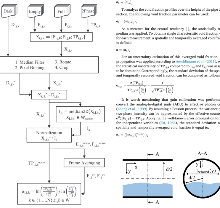
where TPi,j,k, Fi,j and Ei,j are the normalized intensities measured for the two-phase, the pure water (“Full”) and the pure air (“Empty”) opera- tional conditions, respectively. For the full and empty conditions, the intensities are already averaged over all frames whereas the two-phase flow intensity is still frame dependent. The void fraction window W is defined symmetrically to the longitudinal pipe axis with a width, i.e. an extension in the direction of the pipe axis, of 6 mm and a height matching the inner pipe cross-section. A sensitivity study for the void fraction window width was performed. The window width was increased by 60% and reduced by 40%. The resulting absolute deviation of the spatially and temporally averaged void fraction α (cf. equation (9)) from the value obtained at the chosen window size is guaranteed to be smaller than 0.005 for the whole range of operational conditions used in this study. A schematic for the image post-processing and extraction
of the spatially and temporally resolved void fraction αi,j,k is shown in Fig. 5.
For the qualitative analysis of the different flow regimes, averaged void fraction parameters can be deduced from αi,j,k. To examine the global void fraction distribution as a characteristic measure for flow patterns, a spatially weighted average of αi,j,k across the pipe cross- section is calculated in the following way (Pike et al., 1965):
αj,k=∑
i
αi,j,kwchord,i (5)
The chordal weights wchord,i are based on the chord lengths Lchord,i across the tube cross-section as shown schematically in Fig. 6. The chordal weights can be calculated as function of the discrete radial pixel position yi and the inner pipe diameter d:
wchord,i=∑Lchord,i i
Lchord,i
=
̅̅̅̅̅̅̅̅̅̅̅̅̅̅̅̅̅̅̅̅
(d− yi)yi
√
∑
i
̅̅̅̅̅̅̅̅̅̅̅̅̅̅̅̅̅̅̅̅
(d− yi)yi
√ (6)
By averaging over the void fraction window width, i.e. the spatial index j, the temporal dynamics of the flow patterns can be characterized:
αk= 〈αj,k〉j (7)
To analyze the void fraction profiles over the height of the pipe cross- section, the following void fraction parameter can be used:
αi= 〈〈αi,j,k〉j〉k (8)
As a measure for the central tendency 〈⋅〉, the statistically robust median was applied. To obtain a single characteristic void fraction value for each measurement, a spatially and temporally averaged void fraction is defined:
α= 〈αk〉k (9)
For an uncertainty estimation of this averaged void fraction, error propagation was applied according to Aeschlimann et al. (2011), where the statistical uncertainty of TPi,j,k compared to Fi,j and Ei,j was assumed to be dominant. Correspondingly, the standard deviation of the spatially and temporally resolved void fraction can be computed as follows:
σαi,j,k= σ(TPi,j,k
)
TPi,j,kln (
Ei,j Fi,j
)= 1
̅̅̅̅̅̅̅̅̅̅̅
TPi,j,k
√ ln
(
Ei,j Fi,j
) (10)
It is worth mentioning that gain calibration was performed to convert the analog-to-digital units (ADU) to effective photon counts (Zhang et al., 1999). By assuming a Poisson process, the variance of the two-phase intensity can be approximated by the effective counts, i.e.
σ2(TPi,j,k) =TPi,j,k. Applying the well-known error propagation formula for independent variables (Ku, 1966), the standard deviation of the spatially and temporally averaged void fraction is equal to:
σα= 〈〈〈σαi,j,k〉wichord,i〉j〉k (11)
Fig. 5. Schematic of the X-ray post-processing algorithm. Fig. 6. Chord length.
where the chordal weights wchord,i are used for the weighted median with respect to the radial index i. The resulting standard deviation is in the order of 0.05. This is in agreement with previous studies using similar measurement setups (Kendoush and Sarkis, 2002; Pike et al., 1965). The pronounced increase of the statistical uncertainty with a decrease of the void fraction was thoroughly analyzed and discussed by Kendoush and Sarkis (2002). Intuitively, as the void fraction approaches zero, the relative standard deviation of the spatially and temporally resolved void fraction diverges to infinity:
αlimi,j,k→0
σαi,j,k
αi,j,k
= lim
TPi,j,k→Fi,j
1
̅̅̅̅̅̅̅̅̅̅̅
TPi,j,k
√ ln
(
TPi,j,k Fi,j
)=∞ (12)
In addition to the statistical uncertainty, the systematic error due to beam hardening was analyzed using the methodology introduced by Fournier and Jeandey (1984). For the deterministic modelling, the X-ray source spectrum was estimated by the SpekCalc program by Polud- niowski et al. (2009). The mass attenuation coefficients were extracted from the National Institute of Standards and Technology (NIST) stan- dard reference database 126 (Hubbell and Seltzer, 2004). Considering the results from the conducted deterministic simulation, the systematic absolute error induced by beam hardening with respect to the spatially and temporally resolved void fraction αi,j,k is guaranteed to be smaller than 0.007.
4. Results and discussion 4.1. Measurements
In total 13 experiments were performed for an adiabatic upward air–water two-phase flow in the helical coil experimental facility described in section 2. It is assumed that the observed flow process is clearly determined by a finite set of independent operational parame- ters. In case that the geometric boundary conditions and the thermo- dynamic properties are constant, the two-phase flow in a pipe is defined solely by the superficial air and water velocities. This working hypoth- esis assumes further that after a finite entrance length a reproducible flow pattern is developed, which is independent on the flow boundary conditions upstream of the pipe entrance (Saffari et al., 2014). This hydrodynamic developing length is assumed to be shorter than the actual entrance length between the inlet and the measuring position in the experimental facility, which is 5.42 m or a coil length to inner pipe diameter ratio (L/d) of 431. The superficial air and water velocities are calculated by the measured air and water mass flow rates, which were recorded in parallel, but not synchronized, to the X-ray radiography measurements with a total amount of over 100,000 sampling points and a sampling frequency of 1 kHz. The air density was calculated as a function of the measured air temperature (Ta) and two-phase pressure (p) using the ideal gas law. The water density as a function of the measured water temperature (Tw) was obtained by empirical
correlations based on the International Association for the Properties of Water and Steam (IAPWS) IF-97 standard (Wagner et al., 2000). The operational conditions, i.e. the two-phase pressure, the air and water temperatures and the superficial air and water velocities (ja, jw) are summarized in Table 4. The superficial air and water velocities range from 0.18 m/s to 19.5 m/s and from 0.49 m/s to 1.83 m/s, respectively.
The investigated two-phase flows are dominated by inherently sto- chastic turbulent processes. Definition of an appropriate sample size to ensure statistical convergence is therefore essential. A bootstrap based convergence study was carried out. The sample standard deviation of the absolute spatially and temporally averaged void fraction for the number of samples set to 80% of the available sample size is guaranteed to be smaller than 0.004. However, measurement 4 (cf. Table 4) shows a significantly larger standard deviation of 0.015. It may be anticipated that this might be explained by the transitional character of the corre- sponding flow state. The bootstrap samples for representative mea- surements are shown in Fig. 7. In addition, the convergence for sampling continuously, i.e. by maintaining the temporal order of the void fraction array, are presented in Fig. 7 as well. The measurements 1, 3, 7, 9 and 11 were selected randomly as representatives for the individual flow re- gimes and will also be used for the discussion in the succeeding sections.
4.2. Flow regime characterization
According to Zhu et al. (2017), the flow regimes have been classified into six groups, i.e. bubbly, plug, slug, wavy, slug-annular and annular flow. The flow regime assignments for the individual measurements together with the spatially and temporally averaged void fraction values are listed in Table 4 as well. The flow regime identification is based on the X-ray radiography measurements and the resulting void fraction data in form of radiographic void fraction images αi,j,k, histograms to estimate the probability density function (PDF), the void fraction pro- files αi, the void fraction time signals αk and the spatially and temporally averaged void fraction values α. For the histogram, the spatially weighted average of αi,j,k across the pipe cross-section, i.e. αj,k, was used.
A fixed void fraction bin width of 0.01 was applied to ensure compa- rability between the different measurements.
In the following subsections, representative measurement results for the different identified flow regimes are presented and discussed.
4.2.1. Bubbly flow
The measurements 1 and 2 correspond to the bubbly flow regime.
The bubbly flow regime is characterized by small discrete air bubbles within a continuous water phase. The bubbles possess slightly distorted spherical shapes. It is a well know regime and was observed by various helical coil studies presented in the introduction section (Akagawa et al., 1971; Chen and Zhou, 1981; Kaji et al., 1983; Murai et al., 2006; Zhu et al., 2017). The radiographic void fraction image in Fig. 8(a) clearly shows discrete air bubbles, which are predominantly located at the top of the tube. The accumulation of bubbles at the top of the helically coiled Table 4
Experimental measurement results.
Test no. p⋅105 [Pa] Tw [◦C] Ta [◦C] jw [ms−1] ja [ms−1] α ±σα [-] Flow regime
1 1.46 24.4 24.9 1.83 0.18 (1 ±50) ⋅ 10−3 Bubble
2 1.45 24.5 24.8 1.83 0.19 (2 ±50) ⋅ 10−3 Bubble
3 1.55 24.2 25.0 1.77 0.34 (6 ±50) ⋅ 10−3 Plug
4 1.63 23.6 25.1 1.72 0.77 (8.0 ±4.8) ⋅ 10−2 Plug
5 1.76 23.4 25.2 1.64 1.53 (6.18 ±0.46) ⋅ 10−1 Slug
6 1.92 23.2 25.2 1.55 2.46 (7.32 ±0.46) ⋅ 10−1 Slug
7 1.98 23.0 25.2 1.50 2.85 (7.52 ±0.46) ⋅ 10−1 Slug
8 2.39 22.7 25.1 1.20 6.56 (8.13 ±0.46) ⋅ 10−1 Slug
9 2.74 22.5 24.8 0.85 12.2 (8.30 ±0.46) ⋅ 10−1 Slug-Annular
10 2.86 22.4 24.7 0.71 15.2 (8.55 ±0.46) ⋅ 10−1 Slug-Annular
11 2.93 22.2 24.4 0.60 17.5 (8.63 ±0.46) ⋅ 10−1 Annular
12 2.95 22.2 24.3 0.55 18.4 (8.76 ±0.46) ⋅ 10−1 Annular
13 2.99 22.1 24.3 0.49 19.5 (8.83 ±0.46) ⋅ 10−1 Annular
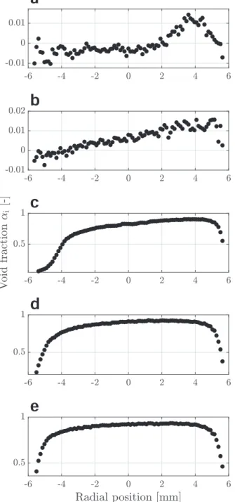
tube due to buoyancy forces was also reported by Zhu et al. (2017). The void fraction profiles over the height of the pipe cross-section charac- terized by αi are shown in Fig. 9 representatively for the six different flow regimes. The radial axis is oriented in upward direction, i.e. the radial position –6 mm indicating the bottom and +6 mm the top of the helical pipe. For the bubbly flow regime, the void fraction close to the top of the pipe is increased due to the accumulation of bigger bubbles as
indicated by the radiographic void fraction image. However, in the middle and lower section of the pipe, the void fraction is close to zero or even negative. As already discussed in section 3.2, this can be explained by the high statistical uncertainty induced by the low void fraction level of this regime compared to the others (Kendoush and Sarkis, 2002). The histograms approximating the probability density functions, i.e. the global void fraction distribution, are presented in Fig. 10 for each flow regime. The bubbly flow in Fig. 10(a) shows a unimodal slightly right skewed distribution peaked at the very low end of the void fraction spectrum caused by the dominant continuous liquid phase present in this regime. The same qualitative results were obtained by Jones and Zuber for vertically oriented straight rectangular channels (Jones and Zuber, 1975). The temporal void fraction dynamics shown in Fig. 11(a) in- dicates a symmetric oscillation. There are a few peaks caused by bigger bubble transits through the void fraction window. It is worth noting that some of the bubbles tend to form clusters, i.e. they flow together in close proximity but without coalescence (cf. Fig. 8(a)). The same was Fig. 7. Statistical convergence. (a) Bubbly flow. (b) Plug flow. (c) Slug flow. (d)
Slug-annular flow. (e) Annular flow.
Fig. 8.Radiographic void fraction images. (a) Bubbly flow. (b) Plug flow. (c) Slug flow. (d) Slug-annular flow. (e) Annular flow.
observed by Zhu et al. (2017). The spatially and temporally averaged void fraction α is smaller than 0.005 for both measurements 1 and 2 (cf.
Table 4).
4.2.2. Plug flow
By increasing the superficial air velocity, the bubbles tend to agglomerate and form elongated Taylor bubbles or plugs, as it can be seen in Fig. 8(b). These plugs are separated by regions of continuous liquid phase with entrained bubbles, which are also known as slugs. The resulting flow regime is defined as plug flow and was detected in the measurements 3 and 4. According to the definition of Zhu et al. (2017), the plug flow is characterized by a spatially and temporally averaged void fraction smaller than 0.5 and a plug length larger than the inner tube diameter. Like for the bubbly flow regime, various studies
investigated the plug flow regime in helical coils (Akagawa et al., 1971;
Liu et al., 2015; Murai et al., 2006; Thandlam et al., 2015; Zhu et al., 2017). As shown in Fig. 9(b), the void fraction profile over the height of the pipe cross-section shows an almost linear increase from the bottom to the top of the tube caused by the varying plug diameters and the staircase shaped tails of the plugs (Conte et al., 2017; Ruder and Han- ratty, 1990). The maximum void fraction is still low due to the domi- nance of the liquid phase, i.e. the plugs are on average much shorter than the slugs. The void fraction based histogram in Fig. 10(b) can be char- acterized by a bimodal distribution with one pronounced peak at the very low end of the void fraction spectrum and one broad peak between 0.2 and 0.6. The lower peak is caused by the slugs whereas the higher peak indicates the plugs. A distinct nearly periodic oscillation between a low and a high void fraction level can be seen in the temporal void Fig. 9. Void fraction profiles over the height of the pipe cross-section. (a)
Bubbly flow. (b) Plug flow. (c) Slug flow. (d) Slug-annular flow. (e) Annular flow.
Fig. 10. Probability density function estimates. (a) Bubbly flow. (b) Plug flow.
(c) Slug flow. (d) Slug-annular flow. (e) Annular flow.
fraction plot in Fig. 11(b). This pattern can be explained by the char- acteristic alternation between plugs and slugs, i.e. the low void fraction level corresponds to the slugs and the high void fraction level to the plugs.
4.2.3. Slug flow
By increasing the superficial air velocity even further, the plugs start to dominate the flow, i.e. the spatially and temporally averaged void fraction gets significantly bigger than 0.5. The slug flow regime shares some similarities with the plug flow regime. The same alternation be- tween the slugs and the plugs characterizes the temporal dynamics of this regime (cf. Fig. 11(c)). In addition, the histogram shows again a bimodal distribution in Fig. 10(c). However, both, the lower and the higher peak are located at slightly higher void fractions and the higher peak now clearly dominates the distribution. This dominance of the gas
phase is also reflected by the void fraction profile over the height of the pipe cross-section in Fig. 9(c). At the bottom of the pipe, a characteristic sigmoid-shaped curve indicates a thick water film, which is present during plug transits. The void fraction profile for the center and the top of the pipe is significantly bigger than 0.5. A sharp drop at the top of the tube indicates a thin water film, which covers the upper wall during plug transits. Additionally, slug flows contain always a high amount of entrained bubbles within the slug. This aeration of the slugs together with potentially enhanced motion blurring due to the higher velocities causes a fuzzy gas–liquid interface at the plug tails as it can be seen in the radiographic void fraction image in Fig. 8(c). In contrast to the plug flow regime, the plug tails are now determined by a hydraulic jump spanning the entire cross-section of the pipe (Conte et al., 2017; Ruder and Hanratty, 1990). Like for the other regimes, this flow regime was observed in various studies performed in helical coils (Akagawa et al., 1971; Banerjee et al., 1969; Chen and Zhou, 1981; Cui et al., 2008; Liu et al., 2015; Murai et al., 2006; Saxena et al., 1990; Thandlam et al., 2015; Zhu et al., 2017).
4.2.4. Slug-Annular flow
The slug-annular flow was reported by only three studies investi- gating flow patterns in vertically oriented helical coils (Akagawa et al., 1971; Banerjee et al., 1969; Zhu et al., 2017). This flow regime is characterized by features from both, slug and annular flows. Similar to the slug flow regime, there is an alternation between plugs and slugs.
During the plug transits in the slug flow regime, there is a thick liquid film at the bottom of the pipe. In the slug-annular flow however, this film is very thin and covers the entire pipe cross-section like in the annular flow regime. The radiographic void fraction image in Fig. 8(d) shows again the tail of a plug. The significantly reduced water phase at the bottom of the tube is clearly visible. The reduced water phase during plug transits is also indicated in Fig. 9(d) by the disappearance of the sigmoid-shaped void fraction profile at the bottom of the tube. The slug transits can be identified in the temporal void fraction evolution plot in Fig. 11(d). The frequency of the slugs is reduced significantly compared to the slug flow regime. Consequently, the low void fraction peak in the probability density function based histogram is even smaller than for the slug flow regime (cf. Fig. 10(d)). In addition, compared to the slug flow regime, the slugs possess a higher characteristic void fraction between 0.4 and 0.5. This increase might be caused by a higher fraction of entrained bubbles in the slugs.
4.2.5. Annular flow
The main characteristic for the transition between slug-annular and annular flow is the disappearance of the slugs. Consequently, as it can be seen in Fig. 8(e), a steady gas core together with a thin water film covering the entire cross-section of the pipe are the dominant flow patterns defining this flow regime. The annular flow was observed in many studies investigating flow patterns in helical coils (Banerjee et al., 1969; Chen and Zhou, 1981; Cui et al., 2008; Kaji et al., 1983; Liu et al., 2015; Whalley, 1980). The void fraction profile over the height of the pipe cross-section shown in Fig. 9(e) is almost symmetrical with respect to the pipe center. Close to the lower and upper pipe walls, the void fraction shows a steep gradient indicating the thin water film present at the walls. Due to the disappearance of the slugs, the temporal void fraction dynamics shows a symmetrical oscillation around the spatially and temporally averaged void fraction (cf. Fig. 11(e)). In addition, the void fraction distribution approximated by the histogram presented in Fig. 10(e) is again unimodal and slightly left skewed with a single peak between 0.8 and 0.9. The unimodality can be explained by the disap- pearance of the slugs, i.e. the liquid phase is only present in form of a thin liquid film at the pipe wall and as entrained droplets in the gas core.
Zhu et al. defined a spatially and temporally averaged threshold void fraction of 0.9 for the transition between the slug-annular and the annular flow regime (Zhu et al., 2017). The experimental results in this study indicate a slightly smaller void fraction threshold between 0.85 Fig. 11. Temporal void fraction dynamics. (a) Bubbly flow. (b) Plug flow. (c)
Slug flow. (d) Slug-annular flow. (e) Annular flow.
and 0.86 (cf. Table 4). This difference could be caused by the different helical coil geometries, especially the significantly larger helix angle of the coil used in this study (cf. Table 1).
5. Conclusions
In this study, high-resolution void fraction measurements were per- formed by means of high-speed X-ray radiography to analyze adiabatic upward air–water two-phase flow patterns in a vertically oriented he- lically coiled tube. The improved post-processing, the decreased expo- sure time and the increased sampling rate of the X-ray radiography system compared to the work of Zhuang et al. (2018) allowed an analysis of various flow pattern details. By using the high-resolution high-speed radiographic void fraction images and several void fraction based fea- tures such as PDF based histograms, void fraction profiles and temporal evolutions, all 13 measurements were classified into five different flow pattern groups, i.e. bubbly, plug, slug, slug-annular and annular flow.
There was no wavy flow observed. According to the results of Zhu et al.
(2017), the wavy regime is expected at significant lower superficial water velocities. The obtained flow regimes are in accordance with flow regime characterizations and transition criteria for helical coils intro- duced by Zhu et al. (2017). Correspondingly, this study supports the findings of earlier studies presented in the introduction section that the intrinsic centrifugal and torsion forces significantly alter the two-phase flow regime transition dynamics in helical coils.
In general, X-ray radiography has proven to be a promising experi- mental technique to investigate flow regimes in helically coiled tubes.
This method provides unique advantages. It is non-invasive as well as non-intrusive. Moreover, no optical access is required, the calibration procedure is simple and the radiographic approach provides global two- dimensional void fraction data in a selected measurement volume. Other techniques such as high-speed imaging or local conductivity probes used in earlier studies are limited to optically accessible features or spatially localized points. Consequently, X-ray radiography is also an ideal experimental technique to validate and improve the predictive capa- bilities of current computational two-phase models (Che et al., 2020).
However, only a limited amount of measurements was carried out in the present study. Further investigations are necessary to analyze the tran- sitions between the flow regimes in more detail, especially at low su- perficial water velocities, and to assess the impact of the helical coil geometry on these transitions. The presented study focuses on adiabatic air–water two-phase flows at ambient conditions. In helically coiled steam generators for advanced nuclear reactors such as the HTGR or NuScale’s SMR design, a water-steam mixture at high pressures and temperatures is used as a coolant within the coils. For such applications, an extension of the operational parameter range towards higher tem- peratures and pressures is recommended. Considering the vast amount of raw data in form of void fraction recordings and the various extractable features, a machine learning approach might be beneficial by providing an objective way to derive flow regime transition criteria and by processing multiple features consistently.
Declaration of Competing Interest
The authors declare that they have no known competing financial interests or personal relationships that could have appeared to influence the work reported in this paper.
Acknowledgments
The work presented herein was supported by the US Department of Energy’s Nuclear Energy Advanced Modeling and Simulation (NEAMS) program as part of the Steam Generator Flow Induced Vibration High Impact Problem.
References
Abouelwafa, M.S.A., Kendall, E.J.M., 1980. The measurement of component ratios in multiphase systems using alpha -ray attenuation. J. Phys. E. 13, 341. https://doi.
org/10.1088/0022-3735/13/3/022.
Aeschlimann, V., Barre, S., Legoupil, S., 2011. X-ray attenuation measurements in a cavitating mixing layer for instantaneous two-dimensional void ratio determination.
Phys. Fluids 23, 1–13. https://doi.org/10.1063/1.3586801.
Akagawa, K., Sakaguchi, T., Minoru, U., 1971. Study on a gas-liquid two-phase flow in helically coiled tubes. Bull. JSME 14, 564–571. https://doi.org/10.1299/
jsme1958.14.564.
Banerjee, S., Rhodes, E., Scott, D.S., 1969. Studies on cocurrent gas-liquid flow in helically coiled tubes. I. Flow patterns, pressure drop and holdup. Can. J. Chem. Eng.
47, 445–453. https://doi.org/10.1002/cjce.5450470509.
Barnea, D., Shoham, O., Taitel, Y., Dukler, A.E., 1980. Flow pattern transition for gas- liquid flow in horizontal and inclined pipes. Comparison of experimental data with theory. Int. J. Multiph. Flow 6, 217–225. https://doi.org/10.1016/0301-9322(80) 90012-9.
B¨aumer, R., Kalinowski, I., R¨ohler, E., Schoning, J., Wachholz, W., 1990. Construction ¨ and operating experience with the 300-MW THTR nuclear power plant. Nucl. Eng.
Des. 121, 155–166. https://doi.org/10.1016/0029-5493(90)90100-C.
Carelli, M.D., Conway, L.E., Oriani, L., Petrovi´c, B., Lombardi, C. V., Ricotti, M.E., Barroso, A.C.O., Collado, J.M., Cinotti, L., Todreas, N.E., Grgi´c, D., Moraes, M.M., Boroughs, R.D., Ninokata, H., Ingersoll, D.T., Oriolo, F., 2004. The design and safety features of the IRIS reactor, in: Nuclear Engineering and Design. North-Holland, pp.
151–167. https://doi.org/10.1016/j.nucengdes.2003.11.022.
Che, S., Breitenmoser, D., Infimovskiy, Y.Y., Manera, A., Petrov, V., 2020. CFD simulation of two-phase flows in helical coils. Front. Energy Res. 8, 65. https://doi.
org/10.3389/fenrg.2020.00065.
Chen, X.-J., Zhou, F.-T., 1981. An investigation on flow pattern transitions for gas-liquid two-phase flow in helical coils, in: 4th International Conference on Alternative Energy Sources. Miami Beach, pp. 69–84.
Cheng, L., Ribatski, G., Thome, J.R., 2008. Two-phase flow patterns and flow-pattern maps: Fundamentals and applications. Appl. Mech. Rev. 61, 050802 https://doi.org/
10.1115/1.2955990.
Chetaland, S.C., Vaidyanathan, G., 1997. Evolution of Design of Steam Generator for Sodium Cooled Reactors, in: 3rd International Conference on Heat Exchangers, Boilers and Pressure Vessels. Alexandria, pp. 41–57.
Conte, M.G., Hegde, G.A., da Silva, M.J., Sum, A.K., Morales, R.E.M., 2017.
Characterization of slug initiation for horizontal air-water two-phase flow. Exp.
Therm. Fluid Sci. 87, 80–92. https://doi.org/10.1016/J.
EXPTHERMFLUSCI.2017.04.023.
Cui, W., Li, L., Xin, M., Jen, T.-C., Liao, Q., Chen, Q., 2008. An experimental study of flow pattern and pressure drop for flow boiling inside microfinned helically coiled tube.
Int. J. Heat Mass Transf. 51, 169–175. https://doi.org/10.1016/J.
IJHEATMASSTRANSFER.2007.04.014.
Dragunov, Y.G., Lemekhov, V.V., Smirnov, V.S., Chernetsov, N.G., 2012. Technical solutions and development stages for the BREST-OD-300 reactor unit. At. Energy 113, 70–77. https://doi.org/10.1007/s10512-012-9597-3.
Fournier, T., Jeandey, C., 1984. Optimization of an experimental setup for void fraction determination by the X-Ray attenuation technique, in: Measuring Techniques in Gas- Liquid Two-Phase Flows. Springer-Verlag, pp. 199–228. https://doi.org/10.1007/
978-3-642-82112-7_12.
Fsadni, A.M., Whitty, J.P.M., 2016. A review on the two-phase heat transfer characteristics in helically coiled tube heat exchangers. Int. J. Heat Mass Transf.
https://doi.org/10.1016/j.ijheatmasstransfer.2015.12.034.
Fsadni, A.M., Whitty, J.P.M., Stables, M.A., 2016. A brief review on frictional pressure drop reduction studies for laminar and turbulent flow in helically coiled tubes. Appl.
Therm. Eng. 109, 334–343. https://doi.org/10.1016/j.applthermaleng.2016.08.068.
Grohse, E.W., 1955. Analysis of gas-fluidized solid systems by x-ray absorption. AIChE J.
1, 358–365. https://doi.org/10.1002/aic.690010315.
Hameed, M.S., Muhammed, M.S., 2003. Mass transfer into liquid falling film in straight and helically coiled tubes. Int. J. Heat Mass Transf. 46, 1715–1724. https://doi.org/
10.1016/S0017-9310(02)00500-8.
Heindel, T.J., 2011. A review of X-Ray flow visualization with applications to multiphase flows. J. Fluids Eng. 133, 074001 https://doi.org/10.1115/1.4004367.
Hubbell, J.H., Seltzer, S., 2004. Tables of X-Ray mass attenuation coefficients and mass energy-absorption coefficients [WWW Document]. NIST Stand. Ref Database 126.
Ingersoll, D.T., Houghton, Z.J., Bromm, R., Desportes, C., 2014. NuScale small modular reactor for co-generation of electricity and water. Desalination 340, 84–93. https://
doi.org/10.1016/j.desal.2014.02.023.
Jones, O.C., Zuber, N., 1975. The interrelation between void fraction fluctuations and flow patterns in two-phase flow. Int. J. Multiph. Flow 2, 273–306. https://doi.org/
10.1016/0301-9322(75)90015-4.
Kaji, M., Mori, M., Nakanishi, S., Ishigai, S., 1983. Flow regime transitions for air-water flow in helically coiled tubes, in: 3rd Multiphase Flow and Heat Transfer Symposium. Miami Beach, pp. 29–30.
Kendoush, A.A., 1992. A comparative study of the various nuclear radiations used for void fraction measurements. Nucl. Eng. Des. 137, 249–257. https://doi.org/
10.1016/0029-5493(92)90023-O.
Kendoush, A.A., Sarkis, Z.A., 2002. Void fraction measurement by X-ray absorption. Exp.
Therm. Fluid Sci. 25, 615–621. https://doi.org/10.1016/S0894-1777(01)00117-0.
Kim, H.K., Kim, S.H., Chung, Y.J., Kim, H.S., 2013. Thermal-hydraulic analysis of SMART steam generator tube rupture using TASS/SMR-S code. Ann. Nucl. Energy 55, 331–340. https://doi.org/10.1016/j.anucene.2013.01.007.