Rapid self-organized criticality: Fractal evolution in extreme environments

(1)

Rapid self-organized criticality: Fractal evolution in extreme environments

Julianne D. Halley,¹ Andrew C. Warden,² Suzanne Sadedin,¹ and Wentian Li³

1School of Biological Sciences, P.O. Box 18, Monash University, Melbourne, Australia 3800

2School of Chemistry, P.O. Box 18, Monash University, Melbourne, Australia 3800

3The Robert S. Boas Center for Genomics and Human Genetics, North Shore LIJ Research Institute, Manhasset, New York 11030, USA (Received 15 October 2003; revised manuscript received 3 May 2004; published 28 September 2004)

We introduce the phenomenon of rapid self-organized criticality(RSOC)and show that, like some models of self-organized criticality (SOC), RSOC generates scale-invariant event distributions and 1 / f noise. Unlike SOC, however, RSOC persists despite more than an order of magnitude variation in driving rate and displays extremely thick and dynamic branching geometry. Starting with an initial set of parameter values, we perform two numerical experiments in which nonequilibrium RSOC systems are tuned towards their critical points. The approach to the critical state is tracked using average branching rates, which must equal 1 if systems are genuinely critical.

DOI: 10.1103/PhysRevE.70.036118 PACS number(s): 89.75.Fb

I. INTRODUCTION

In 1987 Bak, Tang, and Wiesenfeld [1] introduced the theory of self-organized criticality (SOC), which proposed that certain nonequilibrium systems spontaneously evolve to critical states, characterized by power law(fractal)event size distributions and 1 / f noise. The name “self-organized criti- cality” was chosen by the authors to highlight the similarity between SOC systems and criticality in equilibrium systems, and to stress the primary difference between these two types of systems. In both cases, “criticality” refers to the lack of a characteristic scale of internal structures, which are limited only by system size and that of individual units[1–4]. The primary difference between an SOC system and criticality in equilibrium systems is that criticality in the latter is main- tained by the fine-tuning of some control parameter(such as temperature), while criticality in an SOC system apparently self-organizes as energy and matter flow through the system [3–5]. When SOC was introduced, it stimulated enormous interest because of the claim that the theory might help to account for the ubiquity of fractals in space and time(1 / f^⬀ noise) [1,2,4,6,7], one of the oldest puzzles in contemporary physics [8]. SOC was touted as a candidate for a general theory of complexity in nature[4,9], despite the realization that these claims were not wholly correct. Due to a “pro- gramming error”, the square root of the power spectrum was used instead of the power spectrum itself, meaning that the original model of SOC(a numerical sand pile)actually dis- played a 1 / f²signal[10], which is much less interesting than 1 / f noise as 1 / f² signals are easily generated by Brownian motion[11,12]. Although further work revealed that variants of the sand-pile model could show 1 / f noise [13], by then the proposition that SOC was a robust mechanism for 1 / f noise was less convincing. Furthermore, the concept of

“spontaneous” criticality in an SOC system presented several ambiguities[14]. For instance, in most examples of SOC the source of driving was either tuned towards zero or “extremal”[2,6,14,15]. In systems with extremal driving, a glo- bal supervision prevented all but the most extreme sites (rather than statistically typical sites) from receiving inputs of energy[16], an odd state of affairs for self-organized systems [15]. Similarly, several authors noted that tuning the

driving rate towards zero to observe critical fluctuations is hardly self-organized[17].

General theories always elicit healthy skepticism from scientists working in specific fields [2] and self-organized criticality (SOC) is clearly no exception. Although fractals and 1 / f noise can arise in SOC systems, it is apparent that the phenomenon is not as universal as initially claimed and requires some degree of fine-tuning[15,18]. However, recent work on the stick-slip earthquake model revealed that self- organization to an “almost critical” state requires less fine- tuning than the evolution of genuinely criticality, which occurs only at special points in parameter space. Around these points, almost critical dynamics characterizes large regions of parameter space and generates approximate scale invari- ance, which is difficult to distinguish from genuine criticality, unless the average branching rate 共␴兲 is calculated [19,20]. Branching processes must have an average branching rate of 1 to be truly critical[21]. Hence, an SOC system is genuinely critical only if the average branching rate共␴兲of units participating in avalanches equals 1. If ␴⬎1, avalanches are supercritical and expand indefinitely. Conversely, if␴⬍1 the subcritical avalanches invariably expire. A similar pattern was found in a model of Barkhausen noise, which occurs in magnetic materials exposed to external magnetic fields that are ramped up and down. Even though a true power law is found only at a special point in parameter space, the model displays a large critical region[22]. Even in equilibrium, critical fluctuations that overwhelm systems at their critical points remain significant well beyond these points, within so-called “critical regions”[23]. It follows that almost critical dynamics may provide a more realistic expla- nation for the ubiquity of fractals in nature because it is more likely to emerge(and is therefore more robust)than genuine criticality [19,24]. This suggestion is supported by a recent survey of the scaling range of fractals in nature, which found that experimental reports of fractal behavior are usually based on scaling ranges that span only 0.5 to 2 decades[25]. In this paper, we introduce a new type of almost critical dynamics, which emerges when systems are driven rapidly away from equilibrium. We call this phenomenon “rapid self- organized criticality” (RSOC) to distinguish it from other forms of SOC, all of which necessitate driving rates that

(2)

approach zero[2,14,16,26]. Hereafter, slowly driven SOC is referred to as traditional SOC. An important result of this paper is that RSOC generates power law(fractal)event size distributions and 1 / f noise despite more than an order of magnitude variation in driving rate. Indeed, as driving rate is increased RSOC systems become increasingly similar to a critical system, indicated by an average branching rate that approaches 1.

Although in nonliving systems the fine-tuning of specific parameters, such as driving rate, is rare and unlikely[16], in living systems natural selection can be a powerful evolution- ary force. It follows that if there is some benefit associated with criticality (self-organized or otherwise), natural selection might act on control parameters to tune systems towards their critical points [27]. In this paper, we begin with an initial set of parameter values, and perform two numerical experiments in which we progressively fine-tune an RSOC system to obtain an average branching rate共␴兲closer to 1. In the first experiment, we focus on the effects of a variable driving rate, which spanned almost 2 decades. In the second experiment, the driving rate was kept constant while lattice size was increased from 20⫻20 to 80⫻80, a procedure that allowed us to investigate the finite system size effects on model dynamics. The paper is organized as follows. In Sec.

II, we introduce the model and describe statistical methods.

In Sec. III, we present results and in Sec. IV, the main dif- ferences between RSOC and traditional SOC are discussed and conclusions presented.

II. THE MODEL AND DATA ANALYSIS

The inspiration for this work was the feeding behavior of the Argentine ant (Linepithema humile), which uses a pheromone-based mass-recruitment system to communicate the location and quality of food sources[28]. There is often a rapid build-up of ants at high-quality food sources, which become crowded as a result. In a previous study, we found that workers arriving at food sources sometimes disturbed nestmates that were already feeding[29]. These disturbances were slightly autocatalytic, and single wandering ants occa- sionally unleashed avalanches of disturbance, particularly if food sources were crowded and feeding ants were visibly bloated. The distribution of avalanches followed a rough power law distribution over 1 decade[29]. The model presented here is based on this disturbance pattern. However, we are investigating parameter values that are unrealistic for ants, but which allow us to investigate the general phenomenon of RSOC.

Ants are distinguishable by an internal variable, but otherwise behave identically and are created at random sites on lattice borders in a Poisson process at an average rate, ␭ (driving rate of the system). For example, if␭= 10 an average of 10 new ants appear on lattice borders every time step.

While on the lattice, ants are either “wandering” in random walks or “feeding.” Once ants have fed for a total of 460 time steps共t兲, they become “satiated” and wander in random walks until they leave the lattice. The status of each ant is updated once every time step in a “random asynchronous”

manner. In other words, at each time step the population list

(a list comprising all ants on the lattice)is updated, then the status of each ant on the list is updated in random order. At each time step t, an ant is characterized by the following parameters: position on the lattice, feeding status(feeding or wandering), and level of satiation(between 0 and 460 food units). Regardless of driving rate, the average number of ants leaving the lattice equals the average number entering if systems have attained a steady state. At rapid driving rates, systems attain a steady state rather quickly (⬃2500 s for L

= 20, ␭= 1; ⬃18 000 s for L = 80, ␭= 40). In this paper, we are concerned only with steady states, and all data were col- lected after suitable transient periods. The rules of behavior for the model are as follows.

(1) Ants may only move horizontally or vertically to ad- jacent squares on the lattice, not diagonally.

(2) If an unsatiated ant wanders onto an unoccupied square, it will feed at that square until satiated or disturbed, at which point it will wander until it either leaves the lattice or begins feeding again(if not yet satiated).

(3) If an unsatiated ant wanders onto an occupied square, the ant that was feeding at that square will become disturbed and begin wandering, and the first ant will begin feeding at that square.

(4) Both satiated and unsatiated ants will disturb a feeding ant if they wander onto its square.

(5) If two or more unsatiated ants wander onto the same unoccupied square in the same time step, in the next time step one of these ants is selected through the random asynchronous updating process to begin feeding on that square, and the remaining ant(s) continue wandering. If the square was already occupied, then this still applies with the initial occupant of the square being disturbed into a wandering state by the ant that was randomly selected first to feed.

An avalanche propagates through chains of disturbances.

Consider the following:

t A is wandering, B is feeding t + 1 A disturbs B, B stops feeding

t + 2 A feeds, B wanders

t + 3 A feeds, B feeds

This represents the simplest case of an avalanche of magni- tude共s兲= 1, with two participants. An avalanche may propa- gate further as follows:

t A is wandering, B is feeding, C is feeding, D is feeding

t + 1 A disturbs B, B stops feeding t + 2 A feeds, B wanders and disturbs C,

C stops feeding

t + 3 A feeds, B feeds, C wanders and disturbs D, D stops feeding

t + 4 A feeds, B feeds, C feeds, D wanders t + 5 A feeds, B feeds, C feeds, D feeds So, s = 3 with four participants.

A single ant may participate in the same avalanche more than

(3)

once.

t A is wandering, B is feeding, C is feeding, t + 1 A disturbs B, B stops feeding

t + 2 A feeds, B wanders and disturbs C, C stops feeding

t + 3 B feeds, C wanders and disturbs A, A stops feeding

t + 4 C feeds, A disturbs B, B stops feeding t + 5 C feeds, A feeds, B wanders

t + 6 C feeds, A feeds, B feeds, So, s = 4 with three participants.

Note that an ant will also terminate its participation in an avalanche if it wanders off the lattice, and both satiated and unsatiated ants may wander off the lattice.

In a situation where two ants, each participating in different avalanches, both simultaneously wander onto an occupied square and disturb its occupant, the wandering ant whose status is randomly updated first will bring the feeding ant into its avalanche. This is also the ant that will begin feeding at that square, provided it is unsatiated. A satiated ant may single-handedly initiate a large avalanche while wandering back to the lattice boundary, as it can no longer feed at vacant squares. The corresponding probability distribution P共s兲is expected to obey power law behavior with exponent

␶^{, i.e., P}共s兲⬃s⁻^␶[2,30]. Special care was taken to ensure all avalanches were complete before being counted. Note that when the system is driven very rapidly, an excess of wandering ants constantly disturbs the population of feeding ants, resulting in a complex entanglement of social interactions.

Avalanche exponents, which describe how many larger avalanches occur relative to smaller ones, were calculated using linear regressions of log-transformed magnitude and frequency data, so that the upper and lower scales of the model did not affect the calculated exponent(as suggested in Ref.[31]). In the sand-pile model of SOC, the branching rate equals the number of new tumbles directly caused by a tum- bling site[21]. In our model the branching rate of a wandering ant is the number of disturbances it initiates while it is in an uninterrupted bout of wandering. By way of example, consider the following case where ant A is satiated:

t A is wandering, B is feeding, C is feeding, D is feeding

t + 1 A disturbs B, B stops feeding

t + 2 A disturbs C, B wanders, C stops feeding t + 3 A disturbs D, B feeds, C wanders,

D stops feeding

t + 4 A leaves the lattice, B feeds, C feeds, D wanders

t + 5 B feeds, D disturbs C, C stops feeding t + 6 B feeds, D feeds, C wanders

t + 7 B feeds, C disturbs D, D stops feeding t + 8 B feeds, C feeds, D wanders

t + 9 B feeds, C feeds, D feeds

This would give branching rates of: ␴A= 3, ␴B= 0, ␴C1

= 0,␴C2= 1,␴D1= 1,␴D2= 0. The case for A is simple: in the one wandering bout it initiates three disturbances. Similarly, ant B has a single wandering bout but initiates no disturbances. Ant C has two bouts of wandering within the avalanche: during the first bout共t + 2 to t + 4兲, it initiates no disturbances, but in the second wandering bout共t + 5 to t + 8兲 it disturbs ant D. Ant D has two wandering bouts, t + 3 to t + 6 and t + 7 to t + 9. During the first bout it initiates no distur- bances, but initiates one during its second bout. Hence, for this particular avalanche there are six branching rates for four ants. The average branching rate is calculated by sum- ming ␴ for all wandering bouts, then dividing by the total number of wandering bouts, which in this case equals 5 / 6 or approximately 0.83.

Average branching rates for each set of parameter values were calculated using at least 1 million branching rates. Un- fortunately, the rapidly changing dynamics of the model meant that it was not possible to run long simulations for large lattice sizes, as is characteristic for studies on slowly driven SOC. Thus, fast Fourier transforms(FFTs)were based on 16 384共2¹⁴兲time steps, except for the case of L = 70 and L = 80, where 8192 time steps were used. Power spectra s共f兲 were calculated from these FFTs for three variables in each run(the total number of ants, the number of wandering ants, and the number of feeding ants)to establish the presence of 1 / f noise. Power spectra are consistent with 1 / f noise if they behave as 1 / f^⬀, where the exponent ⬀ is between 0.5 and 1.5. White noise and Brownian noise have exponents roughly equal to 0 and 2, respectively [1,32]. Each combination of parameter values was replicated ten times, and averages calculated for all summary statistics.

III. SIMULATIONS AND RESULTS A. Rapid driving

We began with a lattice size of 20⫻20 and ran simulations for driving rates共␭兲of 1, 3, 5, and 10 and then through to␭= 80 (where computer limitations were encountered)in increments of 10. We tracked avalanche response distributions, avalanche exponents, average branching rates, and the power spectra of three variables: the total number of ants in the system, the number of wandering ants, and the number of feeding ants over time.

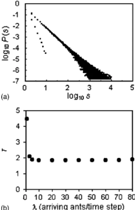
Figure 1(a) displays the probability distribution P共s兲 for systems driven at a rate of 1, 10, 20, 30, 40, 50, 60, 70, or 80 ants/ time step. All distributions overlapped except for␭

= 1, where systems departed significantly from an almost critical state, indicated by a branching rate close to 0.5(see below). When 10艋␭艋80, we find near-perfect overlap of the probability distributions, indicating almost critical behavior over a broad range of driving rates. Figure 1(b), which shows the exponent,␶, of each probability distribution, confirms this result, and Fig. 2 reveals that regardless of driving rate systems of linear dimension L = 20 are invariably sub- critical, indicated by an average branching rate共␴兲that pla- teaus around 0.87± 0.01.

(4)

Analyzing the power spectra of the three variables(total number of ants, number of wandering ants, and number of feeding ants), we find several regions of 1 / f noise. Figure 3 shows the power spectra(averaged across ten replicates)for (a) the total number of ants;(b) the number of wandering ants; and(c)the number of feeding ants over time, for driving rates␭= 1(gray line)and␭= 80(black line). Around 1.5 decades of 1 / f noise were found for both the total number of ants and the number of wandering ants, for all driving rates except ␭= 1. When ␭= 1, the power spectrum of the total number of ants had exponent⬀= 1.67± 0.02, indicating a signal more closely resembling Brownian noise. In contrast, the

exponent of the power spectrum for the total number of ants for driving rates higher than ␭= 1 was around 1.2, well within the 1 / f^⬀ range of 0.5⬍⬀⬍1.5 [1,32]. The power spectrum of the number of wandering ants had an exponent of around 1.3 for all driving rates equal to or greater than 10, while the power spectrum exponent for a driving rate of␭

= 1 was 1.24± 0.03. In addition to the 1.5 decades of 1 / f noise for both the total number of ants and the number of wandering ants for all driving rates greater than ␭= 1, 1 / f noise was also found in the number of feeding ants, but only when the driving rate fell between the bounds 10艋␭艋40.

For driving rates greater than ␭= 40, the signal comprising the number of feeding ants over time increasingly resembled white noise. At the highest driving rate tested 共␭= 80兲, ⬀ FIG. 1. Impact of driving rate on model dynamics. All systems

were 20⫻20 in size and the driving rates␭− 1, 10, 20, 30, 40, 50, 60, 70, or 80 arriving ants/time step were used.(a)Avalanche prob- ability distributions, P共s兲, for the different driving rates. Note that all distributions overlap except for␭= 1 arriving ants/time step.(b) Avalanche probability distribution exponents,␶. Standard errors are not shown because they are smaller than markers.

FIG. 2. Evolution of the average branching rate共␴兲 as driving rate increased from 1 to 80 arriving ants/time step.␴= average average number of disturbances per ant per wandering bout. All systems are 20⫻20 in size. Standard errors are not shown because they are smaller than markers.

FIG. 3. A sample of power spectra S共f兲 for driving rates of␭

= 1 (gray line) or ␭= 80 (black line ). The time signals used in analyses were(a)the total number of ants in systems over time;(b) the number of wandering ants in systems over time; and (c) the number of feeding ants in systems over time. Periodogram values were averaged over ten replicates. Two lines with exponents −1.0 and −2.0 are shown for reference.

(5)

= 0.06± 0.01. In contrast, when␭⬍10, the signal comprising the number of feeding ants closely resembled Brownian noise (at ␭= 1, ⬀= 1.94± 0.03). Although the range of 1 / f noise is limited, the systems studied in this numerical experiment were only 20⫻20 in size. Given this size limitation, the persistence of 1 / f noise in two variables despite more than an order of magnitude variation in driving rate is re- markable.

B. Finite size effects

Finite size scaling theory attempts to predict how long- scale collective phenomena (associated with the onset of fluctuations near critical points)manifest themselves in small samples, such as those commonly used in numerical simulations[33]. Since the theory of SOC suggests that long-range spatial and temporal correlations in nature arise from self- organized dynamics, it is important to investigate how the collective properties of SOC-like models are affected by finite system size.

The second numerical experiment explored how RSOC dynamics is influenced by lattice size, and begins with a lattice size of L = 20. L was then increased in increments of 10 to a maximum of L = 80, at which point computer limita- tions were again encountered. The driving rate remained at

␭= 40 ants/time step throughout this experiment, and avalanche probability distributions, avalanche exponents, average branching rates, and power spectra of the three variables were again calculated.

As system size increased, the magnitude of the largest avalanche observed also increased (⬃4000 for L = 20,

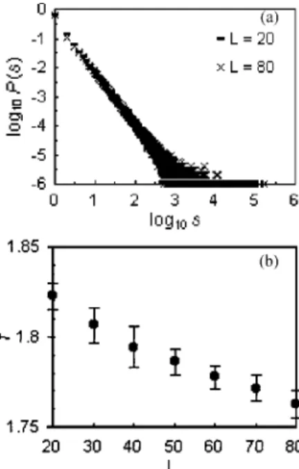
⬃48 000 for L = 40, ⬃92 000 for L = 60, and ⬃170 000 for L = 80). Figure 4(a), which shows the avalanche probability distributions for L = 20 and L = 80, reveals that there is a slight reduction in the slope of the distribution as L increases, suggesting a corresponding reduction in avalanche exponents. Figure 4(b), which plots the avalanche exponent, ␶^, against increasing lattice size, confirms this suggestion. In some previous models of SOC, the avalanche exponent var- ies with the inverse of system size(␶L=␶_⬁^{+ const/ L}[34])or with the inverse of the logarithm of system size (␶L=␶_⬁ + const/ ln L[35]). In these cases, an estimate of the exponent of the infinite system共␶_⬁兲 can be obtained by extrapolation 共L→⬁兲 from data obtained for different values of L. We tried fitting RSOC avalanche exponents at different system sizes to both functions, but were unable to estimate␶_⬁ ^by linear extrapolation. The change in ␶ was more accurately described by the exponential function ␶L= 1.957共1 / L兲^0.024. However, this function suggests that, as L→⬁,␶^approaches zero, a curious result indicating that all avalanche magni- tudes occur with equal frequency at infinite system size.

Clearly, data at larger lattice sizes are needed. Without evi- dence of a limiting value of␶for infinite system size, clas- sification of the universality class of the model is impossible.

Figure 5 shows the average branching rate as a function of the inverse of system size. An excellent fit of these data to the function␴L=␴L⬁+ const/ L facilitates linear extrapolation of the average branching rate to infinite system size. Regres- sion analysis of the transformed data yields an estimate of

␴L⬁= 0.9742± 0.0004, indicating that in the limit of infinite system size, the RSOC system we studied is invariably subcritical. The reason for the subcritical nature of our model may be due to the finite food capacity of individual ants.

After 460 time steps of total feeding time, ants are fully satiated and cannot resume feeding. Such ants regularly disturb the population of feeding(unsatiated)ants as they wander around in random walks.

In the second numerical experiment, regions of 1 / f noise were detected in every set of parameter values. Furthermore, for both the total number of ants and the number of wander- ing ants, the number of decades of 1 / f noise increased from around 2 to 2.5 as lattice size increased from L = 20 to L

= 80[Figs. 6(a)and 6(b)]. The exponents of the power spectra for the total number of ants and the number of wandering ants were similar across all lattice sizes, around 1.3 and 1.4, FIG. 4. Impact of finite system size on model dynamics. (a) Avalanche probability distributions, P共s兲, for lattice sizes L = 20 and L = 80.(b)Avalanche probability distribution exponents,␶, as lattice size(L)increased from L = 20 to L = 80. All systems were exposed to an average driving rate of 40 arriving ants/time step.

FIG. 5. Evolution of the average branching rate␴as lattice size (L) was increased from 20 to 80. ␴= average number of disturbances per ant per wandering bout. All systems were exposed to an average driving rate of 40 arriving ants/time step. Standard errors are not shown because they are smaller than markers.

(6)

respectively. In contrast, the number of decades of 1 / f noise in the number of feeding ants decreased with increasing lattice size, beginning at around 2 decades for a lattice size of 20⫻20, and around 1.5 decades for L = 80. The exponent of the power spectra also changed over this range of lattice sizes(L = 20,⬀= 0.53± 0.02; L = 80,⬀= 1.13± 0.06).

IV. COMPARISON OF RSOC AND TRADITIONAL SOC

Analysis of branching rates indicates that for all systems studied␴⬍1. Such systems are more accurately termed almost critical, not genuinely critical in a mathematical sense.

Nonetheless, all combinations of parameter values led to

power law avalanche distributions over several decades and 1 / f noise was detected in two variables: the total number of ants over time and the number of wandering ants over time.

Although further work is needed to reveal the limits of 1 / f noise and power law avalanche distributions in RSOC systems, these results indicate that fractal formation is surpris- ingly robust with respect to changes in driving rate, a finding that is unique in the study of SOC. It is frequently stated that slow driving is essential for maintaining the effect of thresholds and ensuring a separation of time scales between the source of driving and that of avalanche propagation [2,14,16,36,37]. For example, if the spring-block (earthquake) model is rapidly driven, thresholds associated with springs are constantly overcome and system behavior is dominated by external drive rather than critical dynamics[2]. In our model, there are no obvious thresholds associated with ants or with sites. Instead, feeding ants begin wandering whenever they are contacted by wandering ants, and wandering ants begin feeding spontaneously on unoccupied lattice sites. These two simple features facilitate almost critical dynamics in the face of rapid driving.

Another interesting feature of RSOC is that the largest avalanches can be greater than system(lattice)size. For example, on a lattice of 400 squares共20⫻20兲, the largest avalanche observed for a driving rate of 10 ants/time step was of magnitude 2262. The magnitude of the largest avalanches increased further with increasing driving rate to a maximum of 9208 for a driving rate of 80 arriving ants/time step. This result appears to suggest that rapid driving enables RSOC systems to decouple links between avalanche magnitude and system size. Percolation theory suggests that once interactions span the system, the system is, by definition, critical [38]. However, our branching rate at the limit of infinite system size indicates an inherently subcritical nature for our model, despite avalanches being able to percolate from one end of the system to the other.

Another difference between RSOC and traditional SOC is that in an SOC system, most sites are stable and avalanches are confined to intermittent(effectively instantaneous) periods[39]. Between avalanche events, the system is poised in marginally stable (metastable) states, in which small inputs of energy can trigger arbitrarily large avalanches, possibly as large as the system itself[5]. Thus, the overall behavior of a traditional SOC system comprises a series of isolated avalanche events interspersed by metastable configurations. In other words, each avalanche takes the system from one metastable state to the next[16,37,40]. Such systems have “sparse percolation-like geometry”[2]. In our model, the steady state during which avalanche statistics are stable does not com- prise a series of metastable states. Instead, multiple avalanches are occurring all the time, and local configurations are highly dynamic. Consequently, RSOC gives rise to an extremely thick and dynamic branching geometry.

As well as fractal avalanches, two variables in our model (total number of ants and number of wandering ants) dis- played 1 / f noise as driving rate ranged from 3 to 80 ants/

time step and lattice sizes varied between 20 and 80. Noise with a 1 / f power spectrum is emitted from an astonishing variety of sources, including quasars, sunspots, river flows, and voltage fluctuations across conductors carrying electric FIG. 6. A sample of power spectra S共f兲 for driving rates of␭

= 40 and lattice size L = 20(gray line) and L = 80(black line). The time signals used in analyses were(a) the total number of ants in systems over time;(b) the number of wandering ants in systems over time; and(c)the number of feeding ants in systems over time.

Periodogram values were averaged over ten replicates. Two lines with exponents −1.0 and −2.0 are shown for reference.

(7)

current[12,32,40,41]. Interestingly, 1 / f noise and power law scaling have also been found in electroencephalographic (EEG)recordings and some models of neural network activ- ity, leading several authors to entertain the idea that the human brain is in an SOC state[4,42]. If the brain were subcritical, any input signal could interact with only limited portions of stored information. Conversely, if the brain were supercritical any input would result in explosive branching processes in which new information connects with all previous knowledge[4,43]. In a critical state, however, the brain could be both stable and variable, and may be optimally suited for information processing. This proposal is consistent with the observation that a characteristic feature of normal brains(with or without sensory input)is the background ac- tivity pattern[44]. Unlike transistors, which have their long- est life by remaining inactive, neurons must constantly emit pulses or they atrophy and die. Furthermore, the pulse trains among arrays of neurons must be aperiodic or they eventu- ally entrain, the synchrony becoming manifest as epilepsy [44]. Thus, SOC might play a key role in generating noise and maintaining the health of brain tissue[45].

It is becoming clear that in biological systems, noise can be a useful property [46]. Stochastic resonance is a well- documented phenomenon in which noise is harnessed to in- crease the ability of some nonlinear systems to detect weak signals [47]. Stochastic resonance could play an important role in information processing in both the brain and central nervous system [46,48]. Consequently, the idea that SOC occurs in the brain is receiving increasing attention. How- ever, it is difficult to reconcile the slow driving requirement and “sparse percolation-like geometry” of SOC systems[2] with what is known about the architecture of the human brain. At the height of its development, the human brain has

been estimated to generate several hundred thousand new nerve cells every minute [49], and each of the 10¹¹ or so cortical neurons connects to around 10 000 others [50]. In addition, the dendritic trees of neurons facilitate expansive nonlinear synaptic interactions in many different regions of the tree simultaneously. Such geometry is thought to play a key role in information processing [51], and can hardly be described as sparse. The complex entanglement of interactions is more similar to the rapidly changing dynamics of RSOC systems. The problem of whether RSOC is applicable to neural systems is outside the scope of this paper. Never- theless, we do suggest that RSOC might be a better theory than traditional SOC in understanding brain dynamics.

In summary, we introduce a type of SOC called rapid self-organized criticality(RSOC). Like some models of traditional SOC, RSOC is associated with power law avalanche distributions and 1 / f noise. However, RSOC differs from traditional SOC because it is characterized by an extremely thick and dynamic branching geometry, whereas traditional SOC has been described as having sparse percolation-like geometry[2]. In addition, RSOC can emerge in systems that face extreme nonequilibrium environments, while traditional SOC is overwhelmed in the face of driving rates that rise significantly above zero. Together, SOC and RSOC suggest that the fractal geometry of nature might arise easily through almost critical dynamics.

ACKNOWLEDGMENTS

We thank Ramakrishna Ramaswamy, David Green, Fima Klebaner, Martin Burd, Andreas Schadschneider, Debashish Chowdhury, Charles Osborne, Aidan Sudbury, Imants Svalbe, Peter Wells, Dennis O’Dowd, and Ralph MacNally for helpful comments.

[1]P. Bak, C. Tang, and K. Wiesenfeld, Phys. Rev. Lett. 59, 381 (1987); Phys. Rev. A 38, 364(1988).

[2]T. Gisiger, Biol. Rev. Cambridge Philos. Soc. 76, 161(2001).

[3]H. J. Jensen, Self-Organized Criticality(Cambridge University Press, Cambridge, U.K., 1998).

[4]P. Bak, How Nature Works(Springer-Verlag, New York, 1996). [5]P. Bak and M. Paczuski, Phys. World 6, 39(1993).

[6]S. Clar, B. Drossel, and F. Schwabl, J. Phys.: Condens. Matter 8, 6803(1996).

[7]M. Kardar, Nature(London) 379, 22(1996); D. L. Turcotte, Rep. Prog. Phys. 62, 1377(1999).

[8]J. Davidsen and H. G. Schuster, Phys. Rev. E 62, 6111(2000). [9]M. M. Waldrop, Complexity: The Emerging Science at the

Edge of Chaos(Simon and Schuster, New York, 1992).

[10]H. J. Jensen, K. Christensen, and H. C. Fogedby, Phys. Rev. B 40, 7425(1989).

[11]M. Schroeder, Fractals, Chaos, Power Laws: Minutes from an Infinite Paradise(Freeman, New York, 1991).

[12]J. M. Halley, TREE 11, 33(1996).

[13]K. Christensen, Z. Olami, and P. Bak, Phys. Rev. Lett. 68, 2417(1992).

[14]R. Dickman, A. Vespignani, and S. Zapperi, Phys. Rev. E 57,

5095(1998).

[15]R. Dickman, M. A. Muñoz, A. Vespignani, and S. Zapperi, Braz. J. Phys. 30, 27(2000).

[16]M. Paczuski, S. Maslov, and P. Bak, Phys. Rev. E 53, 414 (1996).

[17]D. Sornette, A. Johansen, and I. Dornic, J. Phys. I 5, 325 (1995); A. Vespignani, S. Zapperi, and V. Loreto, Phys. Rev.

Lett. 77, 4560(1996); J. Stat. Phys. 88, 47(1997); A. Vespig- nani and S. Zapperi, Phys. Rev. Lett. 78, 4793(1997).

[18]V. Frette et al., Nature(London) 379, 49(1996).

[19]O. Kinouchi and C. P. C. Prado, Phys. Rev. E 59, 4964(1999).

[20]J. X. de Carvalho and C. P. C. Prado, Phys. Rev. Lett. 84, 4006 (2000).

[21]C. Adami and J. Chu, Phys. Rev. E 66, 011907(2002).

[22]O. Perkovic, K. Dahmen, and J. P. Sethna, Phys. Rev. Lett. 75, 4528(1995).

[23]P. Ball, Nature(London) 402, C73(1999).

[24]K. Nagel and S. Rasmussen, in Artificial LIfe IV, edited by R.

A. Brooks and P. Maes(MIT Press, Cambridge, MA, 1994).

[25]O. Malcai, D. A. Lidar, O. Biham, and D. Avnir, Phys. Rev. E 56, 2817(1997).

[26]V. B. Priezzhev, D. Dhar, A. Dhar, and S. Krishnamurthy,

(8)

Phys. Rev. Lett. 77, 5079(1996); B. Drossel, Physica A 236, 309(1997).

[27]S. A. Kauffman, The Origins of Order: Self-organization and Selection in Evolution (Oxford University Press, New York, 1993).

[28]B. Hölldobler and E. O. Wilson, The Ants (Belknap Press, Cambridge, MA, 1990).

[29]J. D. Halley and M. Burd, Insectes Soc. 51(3), 226(2004).

[30]S. Lübeck, Phys. Rev. E 62, 6149(2000).

[31]S. D. Edney, P. A. Robinson, and D. Chisholm, Phys. Rev. E 58, 5395(1998).

[32]W. H. Press, Comments. Astrophys. 7, 103(1978).

[33]V. Privman, in Finite Size Scaling and Numerical Simulation of Statistical Systems, edited by V. Privman (World Scientific, Singapore, 1990).

[34]A. Giacometti and A. Díaz-Guilera, Phys. Rev. E 58, 247 (1998); S. Lübeck, ibid. 56, 1590(1997).

[35]S. Lübeck and K. D. Usadel, Phys. Rev. E 55, 4095(1997); S.

S. Manna, Physica A 179, 249(1991); S. S. Manna, J. Stat.

Phys. 59, 509(1990).

[36]R. Sánchez, D. E. Newman, and B. A. Carreras, Phys. Rev.

Lett. 88, 068302(2002).

[37]P. Sinha-Ray and H. J. Jensen, Phys. Rev. E 62, 3215(2000).

[38]G. Grimmett, Percolation, 2nd ed. (Springer-Verlag, New York, 1999).

[39]P. Grassberger, Phys. Rev. E 49, 2436(1994); J. M. Carlson and G. H. Swindle, Proc. Natl. Acad. Sci. U.S.A. 92, 6712 (1995); R. O. Dendy and P. Helander, Phys. Rev. E 57, 3641 (1998).

[40]J. P. Sethna, K. A. Dahmen, and C. R. Myers, Nature(London) 410, 242(2001).

[41]W. Li, Complexity 3, 33(1997); P. Duta and P. M. Horn, Rev.

Mod. Phys. 53, 497(1981); M. B. Weissman, ibid. 60, 537 (1988).

[42]J. J. Hopfield, Physics Today 47, 40(1994); D. Stassinopoulos and P. Bak, Phys. Rev. E 51, 5033(1995); S. Boettcher and M.

Paczuski, Phys. Rev. Lett. 76, 348(1996); Phys. Rev. E 54, 1082(1996); A. R. R. Papa and L. d. Silva, Theory Biosci..

116, 321(1997); L. d. Silva, A. R. R. Papa, and A. M. C. d.

Souza, Phys. Lett. A 242, 343(1998); D. R. Chialvo and P.

Bak, Neuroscience(N.Y.) 90, 1137(1999); G. L. Poupard, R.

Sartène, and J. C. Wallet, Eur. Phys. J. B 12, 303(1999); K.

Linkenkaer-Hansen, V. V. Nikouline, J. M. Palva, and R. J.

Ilmoniemi, J. Neurosci. 21, 1370 (2001); X. Zhao and T.

Chen, Phys. Rev. E 65, 026114(2002).

[43]A. M. Turing, Mind 59, 236(1957).

[44]W. J. Freeman, in Disorder Versus Order in Brain Function:

Essays in Theoretical Neurobiology, edited by P. Århem, C.

Blomberg, and H. Liljenström (World Scientific, Singapore, 2000).

[45]P. Jung, A. Cornell-Bell, K. S. Madden, and F. Moss, J. Neu- rophysiol. 79, 1098(1998).

[46]S. F. Traynelis and F. Jaramillo, Trends Neurosci. 21, 137 (1998).

[47]J. J. Collins, C. C. Chow, and T. T. Imhoff, Nature(London) 376, 236 (1995); K. Wiesenfeld and F. Moss, ibid. 373, 33 (1995); J. J. Collins, ibid. 402, 241(1999); D. F. Russell, L. A.

Wilkens, and F. Moss, ibid. 402, 291(1999).

[48]D. L. Gilden, T. Thornton, and M. W. Mallon, Science 267, 1837(1995).

[49]M. Brown, R. Keynes, and A. Lumsden, The Developing Brain (Oxford University Press, Oxford, 2001).

[50]D. H. Ballard, An Introduction to Natural Computation(MIT Press, London, 1997).

[51]B. W. Mel, in Dendrites, edited by G. Stuart, N. Spruston, and M. Häusser(Oxford University Press, New York, 1999); P. C.

Bressloff and S. Coombes, Int. J. Mod. Phys. B 11, 2343 (1997).