When outcome heterogeneously matters for selection

SFB 823

When outcome

heterogeneously matters for selection: A generalized

selection correction estimator

Discussion Paper Arndt Reichert, Harald Tauchmann

Nr. 40/2012

W HEN O UTCOME H ETEROGENEOUSLY MATTERS FOR S ELECTION : A G ENERALIZED

S ^ELECTION C ^ORRECTION E ^STIMATOR

Arndt Reichert

RWI

Harald Tauchmann

RWI & CINCH^∗

September 2012

Abstract

The classical Heckman (1976, 1979) selection correction estimator (heckit) is misspecified and inconsistent if an interaction of the outcome variable and an explanatory variable matters for selection. To address this specification prob- lem, a full information maximum likelihood estimator and a simple two-step estimator are developed. Monte-Carlo simulations illustrate that the bias of the ordinary heckit estimator is removed by these generalized estimation pro- cedures. Along with OLS and the ordinary heckit procedure, we apply these estimators to data from a randomized trial that evaluates the effectiveness of fi- nancial incentives for weight loss among the obese. Estimation results indicate that the choice of the estimation procedure clearly matters.

JEL codes:C24, C93.

Keywords:selection bias, interaction, heterogeneity, generalized estimator.

∗All correspondence to: Harald Tauchmann, RWI, Hohenzollernstraße 1-3, 45128 Essen, Ger-

1 Introduction

The Heckman (1976, 1979) selection correction (heckit) estimator is a workhorse of applied econometrics, commonly used for removing possible bias due to selection on unobservables.

In many applications, selection into that subsample of obser- vations, for which the outcome variable is observed, may be affected by the value of the outcome variable itself. Think, for instance, of estimating a wage equation.

Here, wages are only observed for individuals who have accepted a wage offer. Yet, the likelihood of accepting the offer increases with the offered wage. Since in the regular heckit estimator, typically, all exogenous variables enter the selection part of the model, the selection equation can be interpreted as a reduced form represen- tation that implicitly captures such impact of outcome on selection.

However, the offered pay may be of differential relevance to different individu- als, e.g., men and women. This renders the effect of the outcome variable on selec- tion heterogeneous with respect to an explanatory variable. In technical terms, this means that not only the outcome variable but also an interaction with the relevant regressor enters the selection model. This, unlike the case of the outcome exert- ing a homogeneous effect on selection, is not accommodated by the regular heckit model. Ignoring the deferential effects of outcome on selection renders the econo- metric model misspecified and, in turn, renders the regular heckit estimator biased and inconsistent.

The present paper develops generalizations of the regular heckit estimator that allows for differential effects of outcome on selection. Besides full information maximum likelihood (FIML), we suggest a computational very simple two-step approach. Overcoming the inconsistency of the ordinary heckit model, the FIML allows for identifying the differential effect of the outcome variable on selection.

The simpler two-step approach is also consistent. However, the coefficient of the interaction term cannot be identified.

We test the performance of the suggested estimators by the means of Monte Carlo simulations. We also apply them to data gathered from a randomized experiment, which was conducted to examine the effectiveness of financial for making obese

1Though it has been criticized for being very vulnerable to various kinds of misspecification (e.g.

Puhani, 2000; Grasdal, 2001), and less restrictive semi-parametric alternatives have been proposed (e.g. Ichimura and Lee, 1991; Ahn and Powell, 1993); see Vella (1998) for a survey.

2The commonly used tobit (type 1) (Tobin, 1958) model represents an extreme case with selection exclusivelydepending on the outcome.

individuals reduce body weight. Here, the incentive scheme makes favorable out- comes more likely to be reported than unfavorable ones, simply by setting stronger incentives to report them. Thus, the suggested link between outcome and the prob- ability of observing the outcome may only exist for the experimental group that is rewarded for success in losing weight.

The remainder of the paper is organized as follows. Section 2 develops the gen- eralized heckit estimators. Section 3 compares the performance of the different esti- mators using a Monte Carlo experiment. Section 4 provides a real data application and Section 5 concludes.

2 A Generalized Heckit Model

Consider a familiar linear regression model, where the focus of the econometric analysis is on estimating the coefficient vector

Y

=

_X

+

_{. (1)}

Here i indexes observations, and Y

,

, and X

denote the outcome variable, a ran- dom error, and the vector of exogenous explanatory variables, respectively. The latter includes the variable D

, which is of special relevance to the analysis, e.g., a treatment indicator.

However, Y

is observed only for a subsample of observation. Selection into this subsample, indicated by S

= 1, is modeled as suggested by Heckman (1979). Yet, besides a K-dimensional vector Z

that includes X

and some further exogenous variables (instruments), Y

as well as the interaction term Y

D

are allowed to enter the selection equation:

S

=

(

1 if

Z

+

+

D

+

> 0

0 else. (2)

As in the ordinary heckit model, joint normality N ( 0, 0,

,

,

) is assumed for

the error terms

and

.

, . . . ,

,

denote unknown coefficients. Substi-

tuting Y

by (1) and rearranging terms leads to S

=

(

1 if

˜

> −

Z

−

X

D

0 else (3)

υ

˜

=

+ (

+

)

, (4) where

=

+

holds for any regressor k that is shared by X

and Z

and

=

holds for the instruments. Evidently, the coefficient

has no impact on the general structure of the model.

For the special case

= 0, (1), (3), and (4) represent the standard Heckman (1979) selection model.

For

6= 0, however, the model deviates from the standard case for two reasons:

(i) a full set of interaction terms X

D

enters the selection equation and (ii), more im- portant, D

enters the error ˜

, rendering the the error variance-covariance structure heterogeneous with respect to D

:

var (

˜

| D

) =

+ 2 (

+

)

+ (

+

)

(5) cov (

, ˜

| D

) =

+ (

+

)

. (6) Ignored heteroscedasticity in the probit and, hence, in the selection part of the heckit, is well known to render probit estimation inconsistent (Wooldridge, 2002;

Harvey, 1976). Thus, a generalized estimator is required.

2.1 FIML Estimation

In oder to develop an estimable FIML estimator that accounts for the model struc- ture, with no loss of generality, we introduce the normalization

σ_υ²

+ 2τσ

+

= 1. (7) That is, we assume standard normality for ˜

conditional on D

= 0. This is equiv- alent to the familiar normalization required for identifying the coefficients of any probit model. We re-parameterize as follows:

ρ

≡ _cor (

_{, ˜}

| D

= ₀ ) =

+

_{. (8)}

3Effectively,τonly changes the unknown error variance-covariance structure, which is subject to estimation. Hence,τis not identified.

Then the individual log-likelihood l

reads as

l

=



















log

√

if S

= 0

log

α⁰Z_i+γβ⁰X_iD_i+(

√

(

)

1−ρ²

−

ε

2

− log

√ 2π if S

= 1.

(9)

See Appendix A.1 for how (9) is derived from the log-likelihood function of the ordinary heckit model. Besides the coefficient vectors

and

, and

are subject to estimation.

Note that D

may either be continuous, a count, or binary.

The model is straightforwardly transferred to the case where the effect of Y

on selection differs across M + 1 mutually exclusive groups, indexed by m = 0, . . . , M.

For group membership being indicated by a set of binary indicators D

, . . . , D

, the log-likelihood conditional on D

= 1 is identical to (9), besides D

is substituted by the value one and

is replaced by

.

Here,

has to be restricted to zero in order to render the model identified.

2.2 Two-Step Estimation

The model (9) is, however, difficult to fit and may cause problems in the optimiza- tion procedure. Yet, for a binary variable D

and, more general, group-wise het- erogeneity, a computationally very simple two-step estimator is available. Here, the heterogeneity in the selection mechanism is accounted for by estimating group- wise probit models at the first stage. For each group m, a specific coefficient vector

is estimated, where the coefficients attached to D

, . . . , D

need to be restricted to the value of zero. At the second stage a vector of group-specific inverse Mills- rations

(·) enter as additional regressors

Y

=

X

+

∑

δmλ

(

ˆ

Z

) D

+

˜

if S

= 1. (10)

4Technically, atanh(ρ)and log(σ_ε)are estimated in the optimization procedure in order to avoid a bounded valid parameter space.

5Typically, all dummiesD_mi, except forD_0iindicating the reference category, enterX_iandZ_i.

The attached coefficients

, subject to estimation, capture

cor (

, ˜

| D

= 1 ) . Two-step estimation comes, however, to the cost of efficiency loss. In the present case, it is not only genuinely less efficient than FIML, like, e.g., the two-step estima- tor for the ordinary heckit model. It also ignores many parameter restrictions that stem from the structural model. For this reason, the two-step approach inflates the number of parameters subject to estimation by M ( K − ₁ ) − _M

. Moreover, (10) may suffer from near-collinearity of correction terms and group indicators. On the other hand, two-step estimating involves less assumptions about the selection mecha- nism than FIML and, hence, also accommodates types of heterogeneity in selection that render (9) misspecified.

3 Monte Carlo Analysis

In order to illustrate the performance of the FIML and the two-step estimators and to compare it with those of ordinary heckit and simple OLS estimation, we run a Monte-Carlo (MC) experiment, where the endogenous variables Y

and S

are gen- erated according to (1) and (2). The exogenous variables, i.e. the vector Z

, are drawn once and then kept fixed. We draw the binary indicator D

from the B ( 1, 0.5 ) distribution and two continuous control variables from the uniform U (− _{1, 1} ) dis- tribution. One of the latter is excluded from the vector X

, while D

enters (2) not only trough Z

but also interacted with Y

. For all coefficients

and

, we choose the value of one, except for the constant terms, which both are set to zero. With respect to the variance-covariance matrix of the normal errors, we choose

= 2,

= 1, and

= 0.75. We vary the experimental setup with respect to: (i)

which we try the values − 1, 0, and 1; and (ii)

consistent with (7), i.e., − 0.75 and 0. The sample size is 10 000 and the size of the simulations is 2 000 repetitions. Our focus is on the estimators’ performance in esti- mating the coefficients

(

^ˆ ) and MSE (

^ˆ ) _.

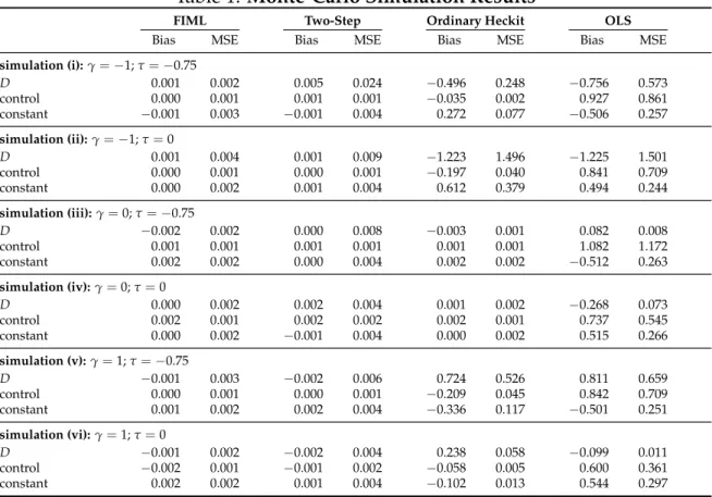
As predicted by theory, MC-results (Table 1) display no significant (warranted by

simulation based tests on joint unbiasedness of ˆ

Step estimator, while OLS is biased in any simulation. Furthermore, the ordinary

heckit estimator does not exhibit a significant bias for

= 0, while it is severely

biased for

6= 0. Focussing on the coefficient attached to D

, depending on the sign

of

6= 0, the ordi-

Table 1:

FIML Two-Step Ordinary Heckit OLS

Bias MSE Bias MSE Bias MSE Bias MSE

simulation (i):γ=−1;τ=−0.75

D 0.001 0.002 0.005 0.024 −0.496 0.248 −0.756 0.573

control 0.000 0.001 0.001 0.001 −0.035 0.002 0.927 0.861

constant −0.001 0.003 −0.001 0.004 0.272 0.077 −0.506 0.257

simulation (ii):γ=−1;τ=0

D 0.001 0.004 0.001 0.009 −1.223 1.496 −1.225 1.501

control 0.000 0.001 0.000 0.001 −0.197 0.040 0.841 0.709

constant 0.000 0.002 0.001 0.004 0.612 0.379 0.494 0.244

simulation (iii):γ=_0;τ=−0.75

D −0.002 0.002 0.000 0.008 −0.003 0.001 0.082 0.008

control 0.001 0.001 0.001 0.001 0.001 0.001 1.082 1.172

constant 0.002 0.002 0.000 0.004 0.002 0.002 −0.512 0.263

simulation (iv):γ=0;τ=0

D 0.000 0.002 0.002 0.004 0.001 0.002 −0.268 0.073

control 0.002 0.001 0.002 0.002 0.002 0.001 0.737 0.545

constant 0.000 0.002 −0.001 0.004 0.000 0.002 0.515 0.266

simulation (v):γ=1;τ=−0.75

D −0.001 0.003 −0.002 0.006 0.724 0.526 0.811 0.659

control 0.000 0.001 0.000 0.001 −0.209 0.045 0.842 0.709

constant 0.001 0.002 0.002 0.004 −0.336 0.117 −0.501 0.251

simulation (vi):γ=1;τ=0

D −0.001 0.002 −0.002 0.004 0.238 0.058 −0.099 0.011

control −0.002 0.001 −0.001 0.002 −0.058 0.005 0.600 0.361

constant 0.002 0.002 0.001 0.004 −0.102 0.013 0.544 0.297

Notes:results based on 2 000 replications; sample sizeN=10 000; exogenous variables drawn once and then kept fixed; true coefficient values:βD=1,β_control=1, andβconst=0.

nary heckit does not perform much better than OLS in terms of the estimated bias.

In simulation (vi), it even perform worse. This means, correcting parametrically for selection bias but misspecifying the selection mechanism may not be an improve- ment compared to simply ignoring selectivity. As expected, Two-Step estimation performs worse compared to FIML, in terms of the estimated MSE.

Even for

= 0 (simulations iii and iv), FIML exhibits an MSE that just marginally exceeds the MSE of the ordinary heckit model.

6For simulations based on a small sample (N = 400), this shortcoming of two-step estimation becomes even more prominent. There, in terms of the MSE, two-step estimation may even be out- performed by the biased ordinary heckit estimator.

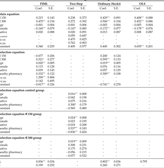
4 Real Data Application

We apply the estimators discussed above to data from a randomized trial; see Au- gurzky et al. (2012) for a detailed description and a comprehensive empirical anal- ysis. This experiment aims at analyzing the effectiveness of financial incentives for assisting obese individuals in losing bodyweight. By the end of a rehab hospital stay, 698 over-weight individuals were set an individual weight-loss target (6 to 8 percent of current body weight), which they were prompted to realize within four months. Participants were then randomly assigned to two incentive groups and one control group. While, contingent on success, a reward of up to

150 and

300, respectively, was offered to members of the incentive groups, the control group re- ceived no financial incentive. Rewards were offered as a function of the degree of target achievement, i.e., participants who lost some weight but failed to realize the weight-loss target received less than the maximum reward. After four months, par- ticipants were requested to visit an assigned pharmacy for verifying actual weight- loss. Yet, a substantial number of participants failed to show up at the weigh-in.

More precisely, 178 individuals selected themselves out of the trial, while 520 com- plied and attended the weigh-in. The compliance rate varied substantially between groups. While for the control group it was 66.5 percent, it was 72.9 and 84.3 per- cent for the

150 and the

300 group, respectively. This nicely meets our earlier argument that the probability of reporting weight is affected by the interaction of actual weight-loss and group membership, as only those who were both successful and members of one of the incentive groups had an financial incentive to attend the weigh-in.

In the present empirical analysis, the degree of target achievement, i.e., actual weight-loss divided by targeted weight-loss, serves as dependent variable. Indi- cators for group membership are the key explanatory variables, with the control group serving as reference. Besides these, age and indicators for being female and being born in Germany enter the regression equation as controls. A further dummy indicating that a participant had to visit a nearby pharmacy, i.e., one within the same zip-code area as the place of residence, exclusively enters the selection equa- tion. This exclusion restriction is justified by travel time representing a likely deter- minant for the decision whether or not to show up at the weigh-in. Yet, there is no obvious link to success.

Table 2 displays regression results for FIML, two-step, ordinary heckit, and OLS.

Table 2:

FIML Two-Step Ordinary Heckit OLS

Coef. S.E. Coef. S.E. Coef. S.E. Coef. S.E.

Main equation:

e150 0.215 0.143 0.238 0.373 0.429^∗∗ 0.091 0.408^∗∗ 0.088

e300 0.470^∗∗ 0.154 0.272 0.392 0.506^∗∗ 0.104 0.452^∗∗ 0.086

age −0.001 0.004 −0.001 0.006 −0.003 0.004 −0.005 0.004

female −0.160^∗∗ 0.079 −0.147^∗ 0.085 −0.172^∗∗ 0.077 −0.178^∗∗ 0.076

native 0.020 0.088 0.020 0.091 0.013 0.087 0.008 0.087

δ_control - - 0.059 0.687 - - - -

δ_e150 - - 0.470 0.425 - - - -

δ_e300 - - 0.762 0.903 - - - -

constant 0.340 0.255 0.409 0.577 0.445 0.302 0.655^∗∗ 0.201

Selection equation:

e150 −0.077 0.206 - - 0.200 0.124 - -

e300 0.521^∗ 0.277 - - 0.595^∗∗ 0.133 - -

age 0.020^∗∗ 0.005 - - 0.019^∗∗ 0.005 - -

female 0.115 0.128 - - 0.076 0.116 - -

native 0.039 0.143 - - 0.057 0.129 - -

nearby pharmacy 0.332^∗∗ 0.122 - - 0.309^∗∗ 0.108 - -

γ_e150 1.206^∗∗ 0.484 - - - - - -

γ_e300 0.142 0.495 - - - - - -

constant −0.817^∗∗ 0.326 - - −0.741^∗∗ 0.278 - -

Selection equation control group:

age - - 0.016^∗∗ 0.008 - - - -

female - - −0.042 0.198 - - - -

native - - 0.075 0.216 - - - -

nearby pharmacy - - 0.300^∗ 0.179 - - - -

constant - - −0.569 0.489 - - - -

Selection equatione150 group:

age - - 0.024^∗∗ 0.008 - - - -

female - - 0.023 0.195 - - - -

native - - −0.018 0.208 - - - -

nearby pharmacy - - 0.537^∗∗ 0.183 - - - -

constant - - −0.836^∗∗ 0.424 - - - -

Selection equatione300 group:

age - - 0.019^∗∗ 0.009 - - - -

female - - 0.308 0.231 - - - -

native - - 0.175 0.274 - - - -

nearby pharmacy - - −0.056 0.215 - - - -

constant - - −0.077 0.522 - - - -

σε 0.836^∗∗ 0.034 - 0.802^∗∗ 0.036 0.795

ρ 0.199 0.252 - 0.260 0.271 -

Notes:^∗∗significant at 5%;^∗significant at 10%; total number of obs. is 698; for 178 obs. weight-loss information is missing.

Test results do not clearly argue for selection bias being an issue since neither for ordinary heckit nor for FIML the estimate for

significantly deviates from zero.

This equivalently holds for the two-step approach, where the group-specific Mill’s ratios are jointly insignificant. Yet, conditional on selection correction, both FIML and two-step are clearly favored over ordinary heckit (p-values 0.03 and 0.01).

Focussing on estimated incentive effects, the choice of estimation method clearly

incentive increases the success rate by roughly 40 to 50 percentage points. Yet, the amount of the financial reward seems to be immaterial for either model. FIML and two-step estimation of the generalized model, however, yield a different picture.

For the latter, no significant incentive effect is seen whatsoever. Here, the ineffi- ciency of two-step estimation is underpinned by rather large standard errors. For FMIL, the estimated incentive effect for the

300 group is similar to ist counterpart from OLS and ordinary heckit estimation. Yet, the estimated effect for the

150 group is substantially smaller and even becomes statistically insignificant. Hence, on basis of FIML, one concludes that the amount of the reward matters for weight loss. The estimates for

and

bear the expected positive sign, however – contrary to expectations –

is much smaller than

and is accompanied by a relatively large standard error, rendering it statistically insignificant. This may be explained by the small number of dropouts in the

300 group, rendering the identification of

difficult.

5 Conclusions

In this article we demonstrate that the classical Heckman (1976, 1979) selection cor-

rection estimator is misspecified and inconsistent when an interaction of the out-

come and an explanatory variables matters for selection. Randomized trials assess-

ing the effects of incentive scheme, may serve as a typical example for such kind

of sample selection mechanism. An FIML and a simple two-step estimator that

address this specification problem are developed. Monte-Carlo simulations illus-

trate that the bias of the ordinary Heckman (1976, 1979) estimator is cured by these

generalized estimation procedures. Finally, the suggested estimators are applied

to data from a randomized trial that evaluates the effectiveness of financial incen-

tives for assisting obese in their attempt for losing bodyweight. Estimation results

indicate that the choice of the estimation procedure clearly matters.

Acknowledgements

This work has been supported in part by the Collaborative Research Center “Statistical Modelling of Nonlinear Dynamic Processes” (SFB 823) of the German Research Foundation (DFG). The au- thors are grateful to “Pakt f ¨ur Forschung und Innovation” and the medical rehabilitation clinics of the German Pension Insurance of the federal state Baden-W ¨urttemberg as well the Association of Pharmacists of Baden-W ¨urttemberg for funding and carrying out data collection. We also like to thank Viktoria Frei, Karl-Heinz Herlitschke, Klaus H ¨ohner, Julia Jochem, Mark Kerßenfischer, Lionita Krepstakies, Claudia Lohkamp, Thomas Michael, Carina Mostert, Stephanie Nobis, Adam Pilny, Margarita Pivovarova, Gisela Schubert, and Marlies Tepaß for research assistance.

References

Ahn, H. and Powell, J. L. (1993). Semiparametric estimation of censored selection models with a nonparametric selection mechanism, Journal of Econometrics

29.

Amemiya, T. (1985). Advanced Econometrics, Harvard University Press, Cambridge, Massachusetts.

Augurzky, B., Bauer, T. K., Reichert, A. R., Schmidt, C. M. and Tauchmann, H.

(2012). Does Money Burn Fat? Evidence from a Randomized Experiment, Ruhr Economic Papers

Grasdal, A. (2001). The performance of sample selection estimators to control for attrition bias, Health Economics

Harvey, A. C. (1976). Estimating regression models with multiplicative het- eroscedasticity, Econometrica

Heckman, J. J. (1976). The common structure of statistical models of truncation, sample selection and limited dependent variables and a simple estimator for such models, Annals of Economics and Social Measurement

Heckman, J. J. (1979). Sample selection bias as a specification error, Econometrica

Ichimura, H. and Lee, L. (1991). Semiparametric least squares estimation of multi- ple index models: Single equation estimation, Vol. 5 of International Symposia in Economic Theory and Econometrics, Cambridge University Press, pp. 3–32.

Puhani, P. (2000). The heckman correction for sample selection and its critique, Journal of Economic Surveys

Tobin, J. (1958). Estimation for relationships with limited dependent variables, Econometrica

Vella, F. (1998). Estimating models with sample selection bias: A survey, Journal of Human Resources

Wooldridge, J. M. (2002). Econometric Analysis of Cross Section and Panel Data, MIT

Press, Cambridge Massachusetts.

A Appendix

A.1 Generalizing the Log-Likelihood Function

In order to generalize the log-likelihood function of the ordinary heckit model (see e.g. Amemiya, 1985, p. 386), we augment the index function

Z

by

X

D

and replace the scalar parameters

and

by the functions (5) and (6), respectively:

l

=































log

−

√

if S

= 0

log









α⁰Z_i+γβ⁰X_iD_i+(Y_i−β⁰X_i)

cov(εi, ˜υ|Di) σ2

ε

s

var(υ˜_i|D_i)

1−^{cov(εi, ˜υi|Di)2}

σ2

εvar(υ˜i|Di)









−

σ_ε

2

− _log

√ 2π

if S

= 1.

(11)

Then we apply the normalization (7) to (5), and eliminate

and

by entering (8) into the equation, yielding

var (

˜

| D

) = 1 + 2γ (

+

) D

+

D

(12)

= 1 + 2ρσ

+

D

,

which is nonnegative, by

being bounded to the [− 1, 1 ] interval. Further, using (6) and, once more, eliminating

and

by entering (8) into the equation yields

cov (

, ˜

| D

)

σ_ε²

=

+ (

+

)

=

σε

+

. (13) Finally, using (13) and (12) we simplify

var (

˜

| D

)

1 − ^cov (

, ˜

| D

)

var (

˜

| D

)

= var (

˜

| D

) −

σε

+

(14)

= var (

˜

| D

) −

− 2ρσ

−

D

= 1 −

,

and substitute (12), (13), and (14) into (11), yielding (9).