No. 619 December 2019
A time-simultaneous multigrid method for parabolic evolution equations
J. Dünnebacke, S. Turek, P. Zajac, A. Sokolov
ISSN: 2190-1767
A time-simultaneous multigrid method for parabolic evolution equations
J. Dünnebacke, S. Turek, P. Zajac, and A. Sokolov
AbstractWe present a time-simultaneous multigrid scheme for parabolic equations that is motivated by blocking multiple time steps together. The resulting method is closely related to multigrid waveform relaxation and is robust with respect to the spatial and temporal grid size and the number of simultaneously computed time steps. We give an intuitive understanding of the convergence behavior and briefly discuss how the theory for multigrid waveform relaxation can be applied in some special cases. Finally, some numerical results for linear and also nonlinear test cases are shown.
1 Motivation
Modern high performance computing systems feature a growing number of proces- sors and massively parallel co-processors, e.g. GPUs, while the performance of each processor does barely increase or even stagnates. To efficiently use such supercom- puters the algorithms have to be massively parallel. The usual time stepping approach to solve time dependent partial differential equations (PDEs) is inherently sequential and does only allow spatial parallelization. If we want to simulate problems with a relatively low number of spatial degrees of freedoms (DOFs), we can only use a certain degree of parallelism, while the number of time steps may be very high due to a long time frame or short time steps. These simulations can not be sped up even if there is more parallel compute power available.
The parallel scalability is limited because the communication between the pro- cesses will outweigh the actual computation time, if too many processes are used.
It is important to note that usually the main cost of the communication stems from Jonas Dünnebacke·Stefan Turek·Peter Zajac·Andriy Sokolov
Institute of Applied Mathematics (LS III), TU Dortmund University, Vogelpothsweg 87, D-44227 Dortmund, Germany
e-mail: {jonas.duennebacke, stefan.turek, peter.zajac, andriy.sokolov}@math.tu-dortmund.de
1
2 J. Dünnebacke, S. Turek, P. Zajac, and A. Sokolov latency and not from limited bandwidth. If the number of communication operations is reduced by communicating more data at once, the scaling behavior can be im- proved, so that more processors can be used efficiently in such simulations (see Fig.
3). To achieve this we have to abandon the sequential time stepping.
There already exists a lot of work on time parallel integration. Many methods are based on integrating ODEs parallel in time. The most prominent examples of this group are Parareal [6] and its variants. Another group of time parallel methods is based on solving a global discrete system with multigrid methods. The first parabolic multigrid was developed by Hackbusch [3]. Other representers of such schemes are the one developed by Horton and Vandewalle [4] as well as the recent variant by Gander and Neumüller [2]. The method our approach resembles the most is multigrid waveform relaxation which was first published by Lubich and Ostermann [7]. For a more complete overview on parallel in time methods, we refer to [1].
2 Time-simultaneous multigrid
In the following, we propose a multigrid scheme that computes many time steps simultaneously but relies solely on spatial parallelization. Here, we start with a second order parabolic evolution equation
𝜕𝑡𝑢(𝑥 , 𝑡) − L (𝑡)𝑢(𝑥 , 𝑡)= 𝑓(𝑥 , 𝑡) (𝑥 , 𝑡) ∈Ω× (0, 𝑇) (1) with suitable initial and boundary conditions.L (𝑡)is a linear elliptic operator for every𝑡 ∈ (0, 𝑇). As discretization schemes we consider linear one- or multistep methods in time and finite element (FE) or finite difference (FD) methods in space so that the discrete linear systems of equations (LSE) can be written as
𝑀
Õ
𝑚=0
𝐴𝑘 , 𝑚u𝑘−𝑚=f𝑘, 𝑘=1, . . . , 𝐾, (2)
with matrices 𝐴𝑘 , 𝑚 ∈R𝑁×𝑁.𝑁 ∈Nis the number of spatial degrees of freedom, 𝐾 ∈Nis the number of time steps and𝑀 ∈Nis the number of steps in the multistep scheme, e.g. 𝑀 = 1 for Crank-Nicolson and Euler schemes or 𝑀 = 𝑅 for linear R-step methods. Then we can gather the time stepping equations (2) in one global system of the form
𝐴1,0
.. .
.. .
𝐴𝑀 , 𝑀−1 . . . 𝐴𝑀 ,0
𝐴𝑀+1, 𝑀 . . . 𝐴𝑀+1,1 𝐴𝑀+1,0
.. .
.. .
.. .
𝐴𝐾 , 𝑀 . . . 𝐴𝐾 ,1 𝐴𝐾 ,0
| {z }
=: ¯𝐴∈R𝑁 𝐾×𝑁 𝐾
u1
.. .
u𝑀
u𝑀+1 .. .
u𝐾
| {z }
=:¯u∈R𝑁 𝐾
=
f1−Í𝑀
𝑚=1𝐴1, 𝑚u1−𝑚
. ..
f𝑀 −𝐴𝑀 , 𝑀u0 f𝑀+1
. ..
f𝐾
| {z }
=:¯f∈R𝑁 𝐾
. (3)
The main idea is to reorder the unknowns from aspace-majorordering
¯
u=[𝑢1,1, . . . , 𝑢1, 𝑁, 𝑢2,1, . . . , 𝑢2, 𝑁, . . . , 𝑢𝐾 ,1, . . . , 𝑢𝐾 , 𝑁]
to atime-majorordering
u=[𝑢1,1, . . . , 𝑢𝐾 ,1, 𝑢1,2, . . . , 𝑢𝐾 ,2, . . . , 𝑢1, 𝑁, . . . , 𝑢𝐾 , 𝑁],
where𝑢𝑘 ,𝑖 = (u𝑘)𝑖 denotes the𝑖-th degree of freedom at the 𝑘-th time step. Re- ordering the right hand side vector¯fand the global matrix ¯𝐴accordingly leads to thetime-blockedsystem matrix𝐴and the vectorf. The Matrix𝐴has the same outer block-structure as the matrices𝐴𝑘 ,𝑙, but each block is a lower triangular𝐾×𝐾matrix with𝑀+1 diagonals.
Now, when we adapt the spatial multigrid method for those systems, we treat each block of the matrix as one entry and use the same transfers and smoothers we would use in a sequential time stepping approach. In our work, we take a Jacobi smoother given by the iteration
u𝑚+1 =u𝑚+𝜔 𝐷−1(f−𝐴u𝑚), (4) where 𝐷 is the block-diagonal part of the reordered matrix 𝐴 and 𝜔 ∈ R is the damping parameter. As we are formally treating the matrix𝐴as a matrix of blocks, we have to use the complete block-diagonal of𝐴to construct the matrix𝐷instead of only using the main diagonal of𝐴. This leads to a block-Jacobi smoother with block dimension 𝐾. Different smoothers that can be written in the form of eq. (4) with different block-matrices𝐷are applicable in the same manner. The transfer operators are constructed by the same reasoning leading tosemi-coarsening in spacewhich means that the transfers in space are applied to each time step independently and the temporal grid stays the same across all levels. With these transfer and smoothing operators the usual multigrid algorithm can be used to solve the LSE incorporating multiple time steps simultaneously.
2.1 Intuitive explanation for small and large time steps
We want to give a short intuitive understanding of two special cases that can help to tweak the algorithm in practice. To do this we consider the one dimensional heat equation. In the most simplistic case of central differences as space discretization and an implicit Euler time discretization the discrete scheme is given by
1 𝜏
(𝑢𝑘 ,𝑖−𝑢𝑘−1,𝑖) − 1 ℎ2
(𝑢𝑘 ,𝑖+1−2𝑢𝑘 ,𝑖+𝑢𝑘 ,𝑖−1)= 𝑓𝑘 ,𝑖 (5) with the (fixed) spatial grid sizeℎand the (fixed) time step size𝜏.
Therefore, the matrix entries belonging to the time derivative are of sizeO (𝜏−1) whereas the values belonging to discrete Laplace operator are of size O (ℎ−2). To
4 J. Dünnebacke, S. Turek, P. Zajac, and A. Sokolov describe the ratio between them we introduce the anisotropy factor𝜆 = ℎ𝜏2 that is widely used in the convergence analysis of space-time multigrid methods [2, 4, 11].
As this parameter depends on the temporal and spatial grids, it changes on dif- ferent levels of the multigrid scheme. Furthermore, it changes locally on each level, if local refinements or space and time dependent diffusion coefficients are used.
Consequently the multigrid method should yield fast convergence for all possible𝜆. In the extreme case𝜆→ ∞the matrix entries belonging to the spatial discretiza- tions prevail. If we ignore the significantly smaller values with a factor of𝜏−1, each block of the global matrix becomes diagonal, so that the global system consists of𝐾 independent𝑁×𝑁systems. Thus, using the time-blocked multigrid is equivalent to solving each time step with a multigrid scheme on its own. This consideration holds true for all BDF-like time discretizations. Other time discretizations show a similar behavior (see Sect. 3). In the opposite case of𝜆&0 the values of the time derivative dominate and therefore the global system becomes block-diagonal, if the mass ma- trix is diagonal. A diagonal mass matrix arises naturally in FD discretizations or can be created by using finite elements with mass lumping. With those block-diagonal matrices the undamped block-Jacobi smoother (𝜔 = 1.0) becomes exact and the multigrid solver converges in one step.
An undamped Jacobi smoother is not a suitable smoother generally and we do not want to choose the damping parameter𝜔based on𝜆manually. Instead, we suggest to use different smoothers, like the Krylov subspace methods BiCGSTAB [9] or GMRES [8] with the block-diagonal matrix𝐷as a preconditioner. These smoothers yield convergence rates similar to the Jacobi smoothing with comparable effort for large𝜆, while they can recover the convergence in one step in the case of𝜆&0 and a diagonal matrix (see Sect. 3).
2.2 Characteristics of the proposed method
The time-simultaneous multigrid scheme can be interpreted as a variation ofmulti- grid waveform relaxation (WRMG) (c.f. [7, 5]). Multigrid waveform relaxation methods are based on discretizing the PDE in space and applying a multigrid split- ting to the stiffness matrix of the semi-discrete ODE system. When using finite elements such a splitting has to be applied to the mass matrix as well to be able to solve the ODEs that arise in every step of the algorithm independently. These methods are equivalent to the time-simultaneous algorithm if a multigrid splitting with a smoother of the form (4) is used for the mass and stiffness matrices and if the same linear multistep method is used to solve every ODE in the multigrid wave- form relaxation scheme. Therefore, we do not provide a more detailed convergence analysis but refer to the literature on WRMG [11, 5].
Remark 1As was shown by Janssen and Vandewalle [5] the time discrete WRMG method for finite elements with a time constant operatorLconverges and yields the same asymptotic convergence rates as the traditional multigrid algorithm in the time stepping case, if the coarse grid system matrix𝐴0and the preconditioning matrices
𝐷𝑙 on each level𝑙 are regular. Due to the equivalence of both methods this result holds true for the time-simultaneous algorithm.
The spectral radius of the iteration matrix is bounded, but that does not imply that the defect reduction in each iteration is bounded as well, since the iteration matrix is not symmetric. For more complex smoothers like BiCGSTAB and GMRES with a time-blocked preconditioner the result mentioned in remark 1 – that is based on the spectral radius of the iteration matrix – cannot be applied, because the resulting multigrid iteration is not linear.
The number of necessary floating point operations (FLOPs) in each iteration of the time-simultaneous method with𝐾blocked time steps is still linear in the number of unknowns𝑁 𝐾. Compared to the time stepping case where a𝑁×𝑁system is solved by a multigrid method in𝐾time steps, the cost of the grid transfer per iteration and time step is the same. The cost of the defect calculation per iteration and time step is slightly higher in the time-simultaneous case, because the global matrix has a higher bandwidth. The application of the block-diagonal preconditioner𝐷in the smoothing operation (4) also has linear complexity, as each block is a lower triangular matrix with𝑀 bands and can be solved by forward substitution.
While the number of required FLOPs of the time-simultaneous method is slightly higher, the number of required communications per multigrid iteration and time step is reduced by a factor of 𝐾−1, because one multigrid solve yields the solution to 𝐾 time steps. Consequently, the latency induced time of the communications can be lowered and better parallel scaling is possible. In order to actually achieve this a telescopic multigrid scheme, where on coarser levels fewer processes are used, needs to be applied. When only a single process is used on the coarse grid, the coarse solve can also be done by time stepping, since no communication is necessary.
The lower triangular solves are inherently sequential, therefore, parallelization in time direction is not trivial. Nevertheless, it is still possible using parallel triangular solvers (c.f. [10]).
To solve non-linear evolution equations we use a time-simultaneous fixed-point or Newton iteration. Using a time stepping scheme we would discretize the equation in time and apply the linearization in each time step, but now we want to solve multiple time steps simultaneously. Therefore, we have to linearize the PDE itself or the global non-linear discrete system.
3 Numerical results
In the following, we provide some exemplary results. As a linear test problem we choose the heat equation
𝜕𝑡𝑢−Δ𝑢=1+0.1 sin(𝑡) (𝑥 , 𝑡) ∈ (0,1)2× (0, 𝑇)
𝑢(0, 𝑡)=𝑢(1, 𝑡)=0 𝑡∈ (0, 𝑇)
𝑢(𝑥 ,0)=0 𝑥∈ (0,1)
6 J. Dünnebacke, S. Turek, P. Zajac, and A. Sokolov with linear finite elements with mass-lumping as space and a Crank-Nicolson scheme as time discretization. The time-blocked multigrid algorithm uses the F-cycle with one block-Jacobi preconditioned BiCGSTAB pre- and post-smoothing step. For each test 1000 time steps were computed using a different number of blocked time steps.
Additionally, we solve the same problem by time stepping and the stationary problem with the same multigrid configuration to create reference results. This was done using spatial grids with grid sizesℎ= 321 andℎ= 1281 . The results are shown in Fig. 1 and 2.
The number of iterations for very small and large time steps behaves as expected.
For𝜆 1 the number of iterations needed to reduce the global defect by a factor of 10−8is independent of the block size and corresponds to the number of iterations that are needed in the stationary test. In the case of𝜆1, the multigrid algorithm converges in one step and in between the number of iteration is at most slightly higher than in the case of large time steps. The only major difference between different block sizes is that the transition area between small and large time steps shifts to smaller time steps if the block size increases.
Comparing the results of different spatial grids shows that the grid size only affects the convergence speed due to its influence on𝜆. Other linear multistep meth- ods, higher order finite elements and different test cases show the same qualitative behavior.
To demonstrate the possible benefits of this approach we show the results of a strong scaling test with the same configuration (see Fig. 3) and grid sizes of ℎ = 1/256 and 𝜏 = 0.001. The method was implemented using theC++ based software packageFEAT31and the tests were executed on the LiDO3 cluster2.
With sequential time stepping the best run time is achievable with 32 CPUs and using more processors yields no benefit. Due to the computational overhead, the time-simultaneous approach needs approximately twice the time for low core counts but provides better scaling. Even with a small block size of 20 time steps, more processors can be efficiently used and the run time can be reduced, but with greater block sizes the time-simultaneous scheme scales even better.
To investigate whether this method can be used for non-linear problems we study the behavior of a time-simultaneous linearization with the one-dimensional viscous Burgers’ equation
𝜕𝑡𝑢−𝜀 𝜕𝑥 𝑥𝑢+𝑢 𝜕𝑥𝑢=0 (𝑥 , 𝑡) ∈ (0,1) × (0, 𝑇) 𝑢(0, 𝑡)=1, 𝑢(1, 𝑡)=0 𝑡∈ (0, 𝑇) 𝑢(𝑥 ,0)=max(1−5𝑥 ,0) 𝑥∈ (0,1)
with the viscosity 0 < 𝜀 ∈ R. Here, we use a FD-discretization with upwind stabilization as discretization in space and Crank-Nicolson in time.
The number of necessary fixed point iteration𝑖𝑡 to achieve a global defect re- duction by 10−6depends on the simulated time frame in the case of small diffusion 1http://www.featflow.de/en/software/feat3.html
2https://www.lido.tu-dortmund.de/
10-5 100 105 0
2 4 6 8
avg. iteration count
stat.
seq.
K=10 K=100 K=1000
10-5 100 105
0 2 4 6 8
avg. iteration count
stat.
seq.
K=10 K=100 K=1000
Fig. 1 Number of iterations in the heat eq. test case with different time step sizes and block dimensions,ℎ=1/32
Fig. 2 Number of iterations in the heat eq. test case with different time step sizes and block dimensions,ℎ=1/128
Fig. 3 Strong scaling test:
Solver time for a increas- ing number of processors, ℎ =1/256 (65536 spatial elements),𝜏=0.001,𝑇 =1 (1000 time steps)
100 101 102 103
#CPUs 100
101 102
solver time
seq.
K=10 K=20 K=100 K=1000
coefficients 𝜀. For example, in the case of𝑇 = 1, 𝜏 = 0.05 and 𝜀 = 10−3 the non-linear solver needs 45 iterations, whereas the averaged number of iterations per time step𝑖𝑡𝑟 𝑒 𝑓 is only 14.25 in the time stepping approach. If the time step size is decreased the number on non-linear iteration in the time stepping case decreases while the global fixed-point iteration does not even manage to converge in 50 steps.
Therefore, a time-simultaneous fixed-point iteration is not suitable for the Burgers’
equation with a small viscosity.
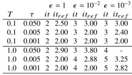
The Newton scheme provides quadratic convergence if the initial guess is close to the solution. Thus, we compute the solution for the same problem with 2ℎ,𝜏and 2𝜀and use it as the initial guess for the simulation with the grid sizes𝜏,ℎand the viscosity𝜀. Using those starting values the number of iterations shows only a slight increase if a longer time frame is calculated simultaneously and in those tests at most 5 iterations are necessary to achieve the desired defect reduction (see Tab. 2).
4 Conclusion
We have presented an algebraic approach leading to a time-simultaneous multigrid method that is closely related to multigrid waveform relaxation. The proposed method
8 J. Dünnebacke, S. Turek, P. Zajac, and A. Sokolov
𝜖=1 𝜖=10−2 𝜖=10−3 𝑇 𝜏 𝑖 𝑡 𝑖 𝑡𝑟 𝑒 𝑓 𝑖 𝑡 𝑖 𝑡𝑟 𝑒 𝑓 𝑖 𝑡 𝑖 𝑡𝑟 𝑒 𝑓 0.1 0.050 4 4.00 10 9.00 13 11.50 0.1 0.005 4 3.00 8 4.15 9 4.45 0.1 0.001 4 2.99 7 3.00 8 3.00 1.0 0.050 5 4.00 23 9.30 45 14.25 1.0 0.005 5 3.00 25 4.92 - 7.42 1.0 0.001 5 2.23 25 3.00 - 4.67
𝜖 =1 𝜖=10−2 𝜖=10−3 𝑇 𝜏 𝑖 𝑡 𝑖 𝑡𝑟 𝑒 𝑓 𝑖 𝑡 𝑖 𝑡𝑟 𝑒 𝑓 𝑖 𝑡 𝑖 𝑡𝑟 𝑒 𝑓 0.1 0.050 2 2.50 3 3.00 3 3.00 0.1 0.005 2 2.00 3 2.00 3 2.40 0.1 0.001 2 2.00 3 2.00 3 2.00 1.0 0.050 2 2.90 3 3.80 4 - 1.0 0.005 2 2.00 4 2.88 5 3.25 1.0 0.001 2 2.00 4 2.00 5 2.82 Table 1 Burgers’ equation: number of fixed-
point iterations,ℎ=20481
Table 2 Burgers’ equation: number of New- ton iterations,ℎ=20481
shows convergence rates that are stable with respect to the number of simultaneous time steps, the grid size and the time step size. The computational cost is slightly higher than in the time stepping case and no parallelization in time direction was done, but the time-simultaneous multigrid method enhances the scalability of the spatial parallelization. The application of this scheme to non-linear equations is also possible by using a time-simultaneous Newton scheme with suitable initial guesses whose choice remains challenging and has to be further examined.
Acknowledgements Calculations have been carried out on the LiDO3 cluster at TU Dortmund.
The support by the LiDO3 team at the ITMC at TU Dortmund is gratefully acknowledged.
References
1. Gander, M.J.: 50 Years of Time Parallel Time Integration. Contrib. Math. Comput. Sci. (2015) doi: 10.1007/978-3-319-23321-5_3
2. Gander, M.J., Neumüller, M.: Analysis of a new space-time parallel multigrid algortihm for parabolic problems. SIAM J. Sci. Comput.38(4), A2173–A2208 (2016)
3. Hackbusch, W.: Parabolic Multi-grid methods. In R. Glowinski and J.-L. Lions (eds.) Com- puting Methods in Applied Science and Engineering VI, pp. 189–197, North-Holland (1984) 4. Horton, G., Vandewalle, S.: A space-time multigrid method for parabolic partial differential
equations. SIAM J. Sci. Comput.16(4), 848–864 (1995)
5. Janssen, J., Vandewalle, S.: Multigrid waveform relaxation on spatial finite element meshes:
The discrete-time case. SIAM J. Sci. Comput.17(1), 133–155 (1996)
6. Lions, J-L., Maday, Y., Turinici, G.: Résolution d’EDP par un schéma en temps «pararéel » (2001) doi: 10.1016/S0764-4442(00)01793-6
7. Lubich, C., Ostermann, A.: Multi-grid dynamic iteration for parabolic equations. BIT Numer.
Math.27(2), 216–234 (1987)
8. Saad, Y., Schultz, M.L.: GMRES: A generalized minimal residual algorithm for solving nonsymmetric linear systems. SIAM J. Sci. Stat. Comput.7(3), 856–869 (1986)
9. Van der Vorst, H.A.: Bi-CGSTAB: A fast and smoothly converging cariant of Bi-CG for the solution of nonsymmetric linear systems. SIAM J. Sci. Stat. Comput.13(2), 631–644 (1992) 10. Vandewalle, S., Van de Velde, E.: Space-time concurrent multigrid waveform relaxation. Ann.
Numer. Math.1(1-4), 347–363 (1994)
11. Vandewalle, S., Horton, G.: Fourier mode analysis of the multigrid waveform relaxation and time-parallel multigrid methods. Computing (1995) doi: 10.1007/BF02238230