Exercise 1: Recap Control Systems I 0 Recap Control Systems I
In this section I’ve resumed all topics and concepts from the courseControl Systems I that are important for Control Systems II as well. This chapter gives one more time the chance to have a look to fundamental concepts.
0.1 System Modeling
A whole course in next semester will be focused on this section (System Modeling).
The normalization and linearization (around the equilibrium x0, u0) of a Model result in the state space description
d
dtx(t) =A·x(t) +b·u(t) y(t) =c·x(t) +d·u(t)
(0.1)
where
A= ∂f0
∂x
x=x0,u=u0
=
∂f0,1
∂x1
x=x0,u=u0
. . . ∂f∂x0,1
n |x=x0,u=u0 ... . . . ...
∂f0,n
∂x1
x=x
0,u=u0
. . . ∂f∂x0,n
n
x=x
0,u=u0
b= ∂f0
∂u
x=x0,u=u0
=
∂f0,1
∂u
x=x0,u=u0
...
∂f0,n
∂u
x=x0,u=u0
c= ∂g0
∂x
x=x0,u=u0
=∂g
0
∂x1
x=x0,u=u0
. . . ∂x∂g0
n
x=x0,u=u0
d= ∂g0
∂u
x=x0,u=u0
=∂g
0
∂u
x=x0,u=u0
The transfer function of the system is given by
P(s) = c(sI−A)−1b+d=bm· (s−ζ1)·(s−ζ2)·. . .·(s−ζm)
(s−π1)·(s−π2)·. . .·(s−πn) (0.2)
• πi are thepoles of the system.
• ζi are thezeros of the system.
Both zeros and poles strong determine the system’s behaviour.
Remark.
• The transfer function does not depend on the chosen system of coordinates.
• Fundamental system properties like stability and controllability, as well.
0.2 Linear System Analysis
0.2.1 Stability (Lyapunov)
Lyapunov stability analyses the behaviour of a system near to an equilibrium point for u(t) = 0 (no input). With the found formulax(t) = x0eAtone can show that Lyapunov stability can be determined through the calculation of the eigenvalues λi of A. The outcomes are
• Stable: ||x(t)||<∞ ∀t ≥0⇔Re(λi)≤0 ∀i
• Asymptotically stable: limt→∞||x(t)||= 0⇔Re(λi)<0 ∀i
• Unstable: limt→∞||x(t)||) =∞ ⇔Re(λi)>0 for at least one i 0.2.2 Controllability
Controllable: is it possible to control all the states of a system with an input u(t)?
A system is said to be completely controllable, if the Controllability Matrix R has full rank
R = b A·b A2·b . . . An−1·b
(0.3) 0.2.3 Observability
Observable: is it possible to reconstruct the initial conditions of all the states of a system from the output y(t)?
A system is said to becompletely observable, if theObservability MatrixO has full rank
O =
c c·A c·A2
... c·An−1
(0.4)
Detectability: A linear time-invariant system is detectable if all unstable modes are observable.
Stabilizability: A linear time-invariant system is stabilizable if all unstable modes are control- lable.
0.3 Feedback System Analysis
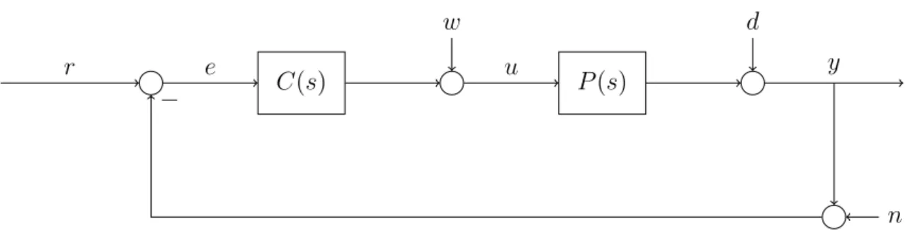
C(s)
w
P(s)
d
r e u y
n
−
Figure 1: Standard feedback control system structure.
The loop gain L(s) is the open-loop transfer function from e→y defined by
L(s) =P(s)·C(s) (0.5)
where P(s) is theplant and C(s) is the controller.
The sensitivity S(s) is the closed-loop transfer function from d→y defined by S(s) = 1
1 +L(s) (0.6)
The complmentary sensitivity T(s) is the closed-loop transfer function from r→y defined by
T(s) = L(s)
1 +L(s) (0.7)
It is quite easy to show that
S(s) +T(s) = 1
1 +L(s)+ L(s)
1 +L(s) = 1 (0.8)
holds. One can define the transfer function of the output signal Y(s) with
Y(s) =T(s)·R(s) +S(s)·D(s)−T(s)·N(s) +S(s)·P(s)·W(s) (0.9) and the tranfer function of theerror signal with
E(s) =S(s)·(R(s)−D(s)−N(s)−P(s)·W(s)) (0.10) whereR(s), D(s), W(s), N(s) are the laplace transforms of the respective signalsr(t), d(t), w(t), n(t).
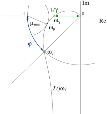
Crossover Frequency
Normally, we want a high amplification at low frequencies for disturbance rejection and a low amplification at high frequencies for noise attenuation.
The crossover frequency ωcis used as reference for the analysis of the system and is defined as the frequency for which it holds
|L(jωc)|= 1 = 0 dB (0.11)
• Bode: Frequency whereL(s) crosses the 0 dB line.
• Nyquist: Frequency whereL(s) crosses the unit circle.
• The bigger ωc is, the more aggressive the system is.
Phase Margin ϕ
180◦±∠L(jωc) (0.12)
• Bode: Distance from -180◦line at crossover frequency ωc. See Figure 2
• Nyquist: Angle distance between the -1 point and the point where L(s) crosses the unit circle. See Figure 3
Gain Margin γ
γ is the inverse of the magnitude of L(jω) if∠L(jω) =-180◦. We call its frequency ωγ,ω∗. 1
γ =|Re(L(jωγ))|, 0 = |Im(L(jωγ))| (0.13)
• Bode: Distance from the 0dB line at frequencyωγ. See Figure 2.
• Nyquist: Inverse of the distance between the origin and the intersection point ofL(s) and the real axis.See Figure 3
You have to think of the phase and the gain margin assafety marginsfor your system. These two are an indicator that tells you how close is the system to oscillation (instability). Thegain margin and the phase margin are the gain and the phase which can be varied before the system becomes marginally stable, that is, just before instability.
This can be seen in Figure 2 and Figure 3.
Figure 2: Bodeplot with phase and gain margin
Figure 3: Nyquist plot with phase and gain margin
0.4 Nyquist theorem
A closed-loop system T(s) is asymptotically stable if nc=n++n0
2 (0.14)
holds, where
• nc: Number of mathematical positive encirclements ofL(s) about critical point−1 (coun- terclockwise).
• n+: Number of unstable poles of L(s) (Re(π)>0).
• n0: Number marginal stable poles ofL(s) (Re(π) = 0).
0.5 Specifications for the closed-loop
The main objective of control systems is to design a controller. Before one does this, one should be sure that the system is controllable. We learned that the controllability and observability are powerful tools to do that, but they are not enough: there are some others conditions for the crossover-frequency ωcthat should be fulfilled for the system in order to design a controller.
It holds
max(10·ωd,2·ωπ+)< ωc < min(0.5·ωζ+,0.1·ωn,0.5·ωdelay,0.2·ω2) (0.15) where
• ωπ+ = Re(π+):Dominant (biggest with Re(π)>0) unstable Pole;
• ωζ+ = Re(ζ+): Dominant (smallest with Re(ζ)>0) nonminimumphase zero;
• ωd: Biggest disturbance-frequency of the system;
• ωn: Smallest noise-frequency of the system;
• ω2: Frequency with 100% uncertainty (|W2(j·ω2)|= 1),
• ωdelay = T 1
delay: Biggest delay of the System.
1 Loop Shaping
1.1 Plant inversion
This method isn’t indicated for nonminimumphase plants and for unstable plants: in those cases this would lead to nonminimumphase or unstable controllers. This method is indicated for simple systems for which it holds
• Plant is asymptotically stable.
• Plant is minimumphase.
The method is then based on a simple step:
L(s) = C(s)·P(s)⇒C(s) =L(s)·P(s)−1 (1.1) The choice of the loop gain is free: it can be chosen such that it meets the specifications.
1.2 Loop shaping for Nonminimumphase systems
A nonminimumphase system shows a wrong response: a change in the input results in a change in sign, that is, the system initially lies. Our controller should therefore bepatient and for this reason we use aslow control system. This is obtained by a crossover frequency that is smaller than the nonminimumphase zero. One begins to design the controller with a PI-Controller.
C(s) =kp ·Ti·s+ 1
Ti·s (1.2)
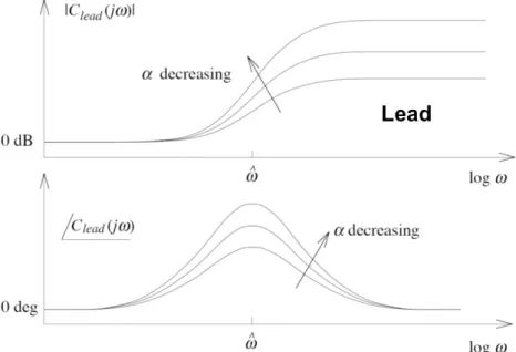
where parameters kp and Ti can be chosen such that the loop gain L(s) meets the known specifications. One can reach better robustness with Lead/Lag elements of the form
C(s) = T ·s+ 1
α·T ·s+ 1 (1.3)
where α, T ∈R+. One can understand the Lead and the Lag as
• α <1: Lead-Element:
→ Phase margin increases.
→ Loop gain’s increases.
• α >1: Lag-Element:
→ Phase margin decreases.
→ Loop gain’s decreases.
Like one can see in Figure 4 and Figure 5 the maximal benefits are reached at frequencies (ˆω) where the drawbacks are not yet fully developed.
The element’s parameters can be calculated as α=
q
tan2( ˆϕ) + 1−tan(ϕ) 2
= 1−sin( ˆϕ)
1 + sin( ˆϕ) (1.4)
and
T = 1
ˆ ω·√
α (1.5)
where ˆω the desired center frequency is and ˆϕ = ϕnew−ϕ the desired maximum phase shift (in rad) is. The classic loop-shaping method reads:
Figure 4: Bodeplot of lead Element
Figure 5: Bodeplot of lag Element
1. Design of a PI(D) controller.
2. Add Lead/Lag elements where needed1
3. Set the gain of the controllerkp such that we reach the desired crossover frequency.
1.3 Loop shaping for unstable systems
Since the Nyquist’s theorem should always hold, if it isn’t the case, one has to design the controller such that nc=n++n20 is valid. To remember is: stable polesincrease the phase by 90◦ and minimumphase zerosdecrease the phase by 90◦
1L(jω) often suits not the learned requirements
1.4 Feasibility
Once the controller is designed, one has to look if this is really feasible and possible to imple- ment. That is, if the number of poles is equal or bigger than the number of zeros of the system.
If that is not the case, one has to add poles at high frequencies, such that they don’t affect the system near the crossover frequency. One could e.g. add to a PID controller a Roll-Off Term as
C(s) = kp·
1 + 1
Ti ·s +Td·s
| {z }
PID Controller
· 1
(τ·s+ 1)2
| {z }
Roll-Off Term
(1.6)
1.5 Examples
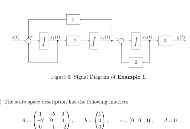
Example 1. The dynamic equations of a system are given as
˙
x1(t) =x1(t)−5x2(t) +u(t)
˙
x2(t) =−2x1(t)
˙
x3(t) =−x2(t)−2x3(t) y(t) = 3x3(t)
(a) Draw theSignal Diagram of the system.
(b) Find the state space description of the above system and write it in Matlab. (c) Find out if the system isLyapunov stable or not, in Matlab.
(d) Find theControllabilitymatrix and determine if the system is controllable in,Matlab. (e) Find the Observability matrix and determine if the system is observable, in Matlab. (f) Find the transfer functionof the system with its poles and zeros, in Matlab
Solution.
(a) The Signal Diagram reads
Figure 6: Signal Diagram of Example 1.
(b) The state space description has the following matrices:
A=
1 −5 0
−2 0 0
0 −1 −2
, b =
1 0 0
, c= 0 0 3
, d= 0
For the rest of solution(b)and solutions(c)-(f )see the attachedMatlabscript: Example_1_EC1.m.
Example 2. Given are a plant P(s) = (s+1)·(s+2)1 and its controller C(s) = (s+1)4 . (a) Compute L(s) and T(s), withMatlab.
(b) Find the gainand the phase margin numerically and plot them, with Matlab. (c) Write the Bodeplot of P(s), C(s), L(s), Matlab.
(d) Write the Nyquistplot of P(s), L(s), with Matlab.
(e) Plot theStep response for the open and closed loop, with Matlab
(f) Plot theImpulse response for the open and the closed loop, with Matlab Solution. See the attached Matlab script: Example_2_EC1.m.