Acknowledgements
First I would like to thank Jun.-Prof. Dr. Birgit Strodel who oered me the possibility to work at such an interesting topic at the Research Center in Jülich and always helped with great suggestions.
Furthermore I would like to thank Dr. Michael Owen who was continuously supporting me through- out my whole work. Thank you for spending so much time and eort to help me nish the thesis successfully.
Moreover, a special thanks goes to the other members of the group, especially Dr. Bogdan Barz, Philipp Kynast, and Qinqhua Liao, who always helped if any technical problems occured.
Finally, a special thanks goes to my family and my boyfriend, René Schimann. Thank you for always standing behind me. And a very special thanks goes to my good friend, Miriam Fabri, for proofreading my thesis and motivating me during the writing process.
Statement
I declare that all material presented in this paper is my own work or fully acknowledged wherever adapted from other sources. I understand that if at any time it is shown that I have signicantly misrepresented material presented here, any degree or credits awarded to me on the basis of that material may be revoked.
I declare that all statements and information contained here are true, correct and accurate to the best of my knowledge and belief.
Ort, Datum Unterschrift
Contents
1 Introduction 2
2 Molecular Dynamics 6
3 Methods 9
3.1 The Program and Parametrization . . . 9
3.2 Analysis Methods . . . 10
3.2.1 Dene Secondary Structure of Proteins . . . 10
3.2.2 Root Mean Square Deviation . . . 11
3.2.3 Radius of Gyration . . . 11
3.2.4 Cluster Analysis . . . 12
4 Results 13 4.1 DSSP . . . 13
4.2 Secondary Structure as a Function of Residue . . . 18
4.3 Radius of Gyration and RMSD . . . 23
4.4 Cluster Analysis . . . 26
5 Discussion 32 5.1 Secondary Structure . . . 32
5.2 Radius of Gyration and RMSD . . . 33
5.3 Cluster Analysis . . . 34
6 Conclusion and Prospects 35
7 Appendix 37
1 Introduction
Alzheimer's disease (AD) is a neurological disorder for which there is no known cure [1]. In 2010 there were 35.6 million people living with the dementia worldwide. This number is projected to increase to about 65.7 million by 2030 and 115.4 million by 2050 [2].
Patients suering from AD lose cognitive and functional abilities. In most cases the disease occurs among the elderly. The most common and early symptom is the loss of the short-term memory. As AD proceeds the patients show more symptoms such as confusion, aggression, and long-term memory loss. The brain of AD patients looks very dierent from healthy brains. A massive loss of neurons occurs in the brain. The cortex, which is involved in thinking, planning and remembering, shrinks. The hippocampus is strongly aected. The hippocampus is important for the formation of new memories which leads to the loss of the short-term memory. The uid- lled spaces within the brain, called ventricles, grow larger. The brain tissue of an AD brain shows much fewer nerve cells and synapses under a microscope than a healthy brain does [3].
In addition to cell loss, plaques also forme in the AD brain. Extracellular plaques are clusters of aggregated amyloidβ-peptides (Aβ) [4]. It is assumed that plaques are not the most toxic state of the Aβ peptides, but rather that the smaller oligomers of Aβ are more toxic [1]. Another cause of the disease might be the formation of intracellular neurobrillary tangles. This occurs when the protein tau forms twisted strands. The result of plaque and bril formation might be a malfunction of the biochemical communication between neurons, which nally leads to the death of the cells.
The minority of AD cases are caused by genetic errors, also called familial AD. Aβ (Figure 1) is a peptide generated in the brain and peripheral tissues. It is believed to be an incidental catabolic byproduct of the amyloid precursor protein (APP) [4]. However APP can serve as a ligand for dierent receptors and molecules. APP is an integral membrane protein. Its funtion is not completely known, but it is assumed that it plays a role in the regulation of synapse formation.
The APP is cleaved by two dierent enzymes, theβ-secretase and theγ-secretase, which leads to the formation of Aβ40 and Aβ42, where Aβ40 has 40 amino acids and Aβ42 has 42 amino acids [4].
Aβ40 is the predominant form of Aβ in the human brain [5]. In normal metabolism these proteins are generated continuously but they do not deposit in the brain.
Figure 1: Illustration of Aβ42 (pdb-code: 1Z0Q) The Figure was generated by the program Vi- sual Molecular Dynamics (VMD). The representation was done with the New Cartoon drawing method. The coloring method was Secondary Structure. The N-terminus and the C-terminus are representend by the red and blue beads, respectively.
In principle the Aβ hypothesis states that the formation of plaques, caused by the aggregation of Aβ, is the fundamental cause of AD. Aβ42 contains two more hydrophobic amino acids than Aβ40. Therefore the aggregation of Aβ42 happens much faster. When the peptides are aggregated they form beta-sheets. The extracellular plaques are not soluble. But there are some suggestions that the smaller soluble oligomers that are also found in the cells are far more toxic, since some symptoms of AD appear before plaques are formed. However there are people that have Aβ deposits in their brain, but do not show any symptoms. A possible explanation of this is that too much Aβ changes the activity of kinases and phosphatases.
AD is thought to be related to severe oxidative stress [6]. Oxidative stress occurs when the production of oxygen-containing reactive compounds, such as the super peroxide anion (O2−•), hydrogen peroxide (H2O2), or hydroxyl radicals (OH•) is increased. Normally oxidative and reductive species are balanced inside the cells. In the case of oxidative stress the oxidative species are predominant. This imbalance causes cellular damage. Hydrogen peroxide can diuse long distances by crossing membranes and cause damage in regions from its site of origin. Hydroxyl radicals, however, are much more reactive. They react with almost any biological compound, causing damage at the rst molecule it collides with [7]. Radicals in a cell will cause damage at lipids. They can also react with fatty acids, causing them to dimerize .
Oxidative damage might even be caused by Aβ itself. Aβ is capable of generating hydrogen peroxide by reacting with copper- and iron-ions. Copper, iron and zinc have dierent eects on the
toxicity of Aβ. Copper causes and zinc inhibits the toxicity of Aβ [8]. While Cu2+ and Fe3+ are reduced by Aβ, the reaction generatesH2O2and peptide radicals (Aβ+•). Both, copper and iron, can be reduced by Aβ. Aβ brils are able to generateH2O2 directly from molecular oxygen [4].
Cu2+ binds to Aβ. The reaction that occurs is a redox reaction, converting molecular oxygen into hydrogen peroxide. In the brain of AD patients the concentration of Fe2+ is higher than it is in healthy brains. Therefore the Fenton reaction can take place. Fe2+ reacts with H2O2 to generate hydroxyl ions and hydroxyl radicals. Hydroxyl radicals can also be generated by heat and ionization radiation.
On peptides,α-carbons (Cα) are the thermodynamically favorable positions for the hydrogen- abtraction (H-abstraction). In the case of Aβ, the generation of the radical occurs at the side chain of the methionine residue, afterwards the radical is relocated to glycine residues. The radicals, positioned onα-carbons, play an important role in oxidative damage, because they are stabilized by the captodative eect [9]. This eect is a result of the combined action of electron-drawing groups (acceptors or captors) and electron releasing groups (donors) [5]. Radicals on Aβ will be favored on certain residues [10]. Due to steric reasons it is probable that radicals will be generated on glycine or alanine residues. However it has been shown that the H•abstraction from the Cαof glycine is three times faster than it is from the Cαof alanine [11].
Often one talks about aqueous surroundings when refering to proteins. This is justied due to the fact that the body consists of more than 60% water. But next to water, there are other molecules, such as proteins, lipids, or minerals [12], in the cell as well that decrease the hydrophilic properties of the cell. These components can aect the structure of peptides and proteins, therefore non-aqueous solvents should also be used to mimic the environment of the cell.
Many proteins or peptides interact with lipids. Certain solvent systems, such as water/uorinated alcohol mixtures can represent a possible model to reproduce the hydrophobic/hydrophilic charac- ter of the membrane surface and the surroundings in a cell [13]. The eects of uorinated alcohols on proteins and peptides were strongly analyzed over the last few decades [14]. Triuoroethanol (TFE), for example, has an inuence on the hydrophobic eect [15]. Therefore it is more realistic to study Aβ not only in water, but in water/alcohol mixtures, such as water/TFE. The eect of TFE on the conformation of peptides can be studied by varying the concentration and comparing the results to a system that does not contain TFE.
Experimental studies of Aβ are possible, but not easy. In water, the peptide is not folded and it aggregates simply too fast. The process of folding, unfolding, forming of β-sheets, as well as the aggregation process cannot be examined experimentally. This process can be visualized by molecular dynamic (MD) simulations. The main advantage of this theoretical method is that it
allows to gain insight into processes, such as folding and unfolding of proteins or protein-protein interactions.
This thesis has the aim to understand the eect of glycine radicals on the conformation of amyloid-β peptide. Based on the results, aggregation studies can be done by studying the eect of glycine radicals on the aggregation process of Aβ.
2 Molecular Dynamics
The basic principle of MD simulations follows Newton's second law of motion:
F~ =m·~a (1)
The forceF~ is equal to the change in momentum~pwith a change in time. Momentum is dened to be the massmof an object times its velocity~v. The mass does not change as it moves, so the equation can be simplied to massmmultiplied by the rate of change of velocity, which is called acceleration~a:
F = ∂~p
∂t =m∂(~v)
∂t (2)
A system with N paticles gives a set of 3N rst-order dierential equations:
miv˙i,a=−∂U(R)
∂ri,a (3)
where
i = 1, ..., N and a = x, y, z and R = {r1,x, r1,y, r1,z, ..., rN,x, rN,y, rN,z} indicates the Cartesian vector of the positions of the particles.
U(R)is the potential energy, andvi,a is the velocity of particle i in x, y and z direction.
To perform classical MD simulations, Equation 3 has to be solved. To solve it, it has to be integrated numerically.
To numerically solve the problem, a time step∆t >0 is chosen and the sampling point sequence tn =n∆t is examined. The duty is to nd a sequence of pointsRn that follow the points R(tn) on the trajectory of the exact solution.
All integration algorithms assume that the positions, velocities, and accelerations can be approxi- mated by a Taylor series expansion. The algorithm used in this work is the Leapfrog algorithm [16]:
v
t−∆t 2
≡ r(t)−r(t−∆t)
∆t (4)
v
t+∆t 2
≡ r(t+ ∆t)−r(t)
∆t (5)
The velocities v t+∆t2
are rst calculated via a Taylor series expansion. These are used to calculate the positionsr at timet+ ∆t:
v
t+∆t 2
≈v
t−∆t 2
+ ∆tF(t)
m (6)
r(t+ ∆t)≈r(t) + ∆tv
t+∆t 2
(7) where
vis the velocity, andt is the time.
F(t)is the force,mis the mass andris the position.
This way the velocities leap over the positions, then the positions leap over the velocities. The main advantage is that the velocities are calculated explicitly. The disadvantage, on the other hand, is that the velocities and the positions are not dened at the same time. Because of that, the kinetic and potential energy are also not dened at the same time. Therefore, in the leap frog scheme, the total energy is not calculated directly.
During the simulation, Newton's second equation of motion is solved for every time step. The potential energy term consists of bonded and nonbonded contributions. Bonded contributions result from bond length displacement, bond angle bending and torsion angle rotations. Nonbonded interactions result from electrostatic and van der Waals interactions.
The total energyUtotof a molecular system is the sum of the energy of the various components:
the nonbonded energyUnb, the bond stretchingUbond, angle bendingUangle, and torsional rotation Utorsion. In this work, the OPLS-AA force eld was employed [17]. Thus the equations for the OPLS-AA force eld are provided in the following.
The bond stretching and angle bending energies are described by Equations 8 and 9:
Ubond= X
bonds
Kr(r−req)2 (8)
Uangle= X
angles
KΘ(Θ−Θeq)2 (9)
where
ris the bond length Θis the bond angle
req andΘeq are the equilibrium values for the bond length and bond angle, respectively Kr andKΘare the force constants
The term for the torsion energy is described by Equation 10:
Utorsion = X
torsions
V1i
2 [1 +cos(φi)] +V2i
2 [1−cos(2φi)] +V3i 2
1 +cos(3φi)
(10) where
V1i,V2i,V3i indicate barriers for the torsional motion.
The summation is performed over all of the dihedral anglesφi.
The nonbonded energy term of the force eld is described by Equation 11. It is the sum of the Coulomb and Lennard-Jones contributions for pairwise intra- and intermolecular interactions.
Unb=X
i<j
"
qiqje2 rij + 4ij
σ12ij r12ij −σij6
rij6
!#
fij (11)
where
qi andqi are partial atomic charges for atomsiandj,eis the unit charge, andrij is the distance between atomsiandj.
σandare the Lennard-Jones coecients. Forσij andij the combining rulesσij =√
σiiσjj and ij=√
iijj were employed [18].
fij is an interaction coecient. It is equal to 0.0 for anyij pairs connected by a valence bond (1-2 pairs) or a valence bond angle (1-3 pairs). j ) 0.5 for 1,4 interactions andfij is equal to 1.0 for all other cases.
The nal force eld equation can be combined to form Equation 12:
U(R) = X
bonds
Kr(r−req)2+ X
angles
KΘ(Θ−Θeq)2
+ X
torsions
V1i
2 [1 +cos(φi)] +V2i
2 [1−cos(2φi)] +V3i 2
1 +cos(3φi)
+ X
nonbonded
"
qiqje2 rij
+ 4ij σij12 rij12 −σ6ij
r6ij
!#
(12)
3 Methods
The MD simulations were done using gromacs version 4.6.5 [19] and the opls-aa force eld [17].
The following section gives more detailed information about the parametrization of the 16 simula- tions that were done.
3.1 The Program and Parametrization
To perform molecular dynamics simulations on peptides that contain a radical using gromacs, the program had to be slightly modied. For gromacs to recognize GLR as the radicalized form of glycine (Gly), this information had to be provided for the force eld. The parameters were already developed by Komáromi et al. [20] for the opls-aa force eld, which is why this force eld was used to perform the MD simulations.
For all simulations the same starting structure of Aβ42 was used. The structure 1Z0Q was taken from the rcsb protein data bank. The pdb le was modied as well, so that it contained the glycyl radical residue in dierent positions, namely at residues Gly-25, Gly-29, or Gly-33. Each of the peptides was placed in a cubic box with an edge length of 1.5 nm. Moreover, periodic boundary conditions were used. Then water (tip4p water model) was added, before the system was neutralized by adding chloride ions. Finally, sodium chloride was added to the system, so its concentration was 0.15 moll .
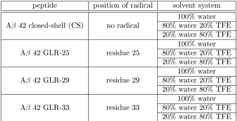
First, the four Aβ peptides were simulated for 100 ns. During these simulations, a total of 5107 integration steps, with a step size of 2 fs, were performed. Three dierent solvent systems were used, as Table 1 states: rst 100% water, second 80% water and 20% TFE in combination, and third 20% water and 80% TFE in combination. In the remainder of this work, the solvent system, consisting of 80% water and 20% TFE will be meant by 80% water. The system of 20% water and 80% TFE will be called 20% water.
Table 1: MD Simulations that were performed for 100 ns peptide position of radical solvent system Aβ 42 closed-shell (CS) no radical 100% water
80% water 20% TFE 20% water 80% TFE
Aβ 42 GLR-25 residue 25 100% water
80% water 20% TFE 20% water 80% TFE
Aβ 42 GLR-29 residue 29 100% water
80% water 20% TFE 20% water 80% TFE
Aβ 42 GLR-33 residue 33 100% water
80% water 20% TFE 20% water 80% TFE
The simulations were done using the isothermic-isobaric ensemble (NPT). The temperature coupling was via the Berendsen thermostat [21], and the pressure coupling was via the Parrinello- Rahman barostat [22]. The simulations were performed at 300 K and 1 bar. The non-bonded interactions were calculated using the Particle-Mesh-Ewald method. The short-range cuto of the electrostatic (Coulomb) interaction was 0.9 nm, the short-range van der Waals cuto was 1.4 nm.
The minimization was performed by the steepest-descend method, with 1000 minimization steps.
The integration of Newton's second equation of motion was done by the Leapfrog algorithm.
A later analysis of the simulations showed eects that were only present when TFE was used as a co-solvent. Due to this, the simulations in water were extended for 400 ns to see if the eect appears as well in water if the sampling time is increased. The parameters were kept the same for the extention.
3.2 Analysis Methods
3.2.1 Dene Secondary Structure of Proteins
The Dene Secondary Structure of Proteins (DSSP) is a method gromacs uses to plot the sec- ondary structure as a function of time and residue. The program uses a recognition algorithm for secondary structure. It is based on H-bonding patterns [23]. The algorithm recognizes so called turns with an H-bond between the carbonyl group (CO) of residue i and the amino group (NH) of residue i+n, where n= 3,4,5. The algorithm recognizes other interactions called bridges, with an H-bonds between residues that are not close to each other in sequence (n >5).
The hydrogen bonds in proteins are described by an electrostatic model [24]. The DSSP pro- gram calculates the electrostatic interaction energy (kcalmol) between two H-bonding groups by ap- plying partial charges on the CO group and the NH group.
E=q1q2
1
r(ON)+ 1
r(CH)− 1
r(OH)− 1 r(CN)
f (13)
where
q1= 0.42eandq2= 0.20e, e is the unit charge
r(AB)is the interatomic distance betweenAandB in Angstroms f = 332is the dimensional factor, its unit is kcalmol.
The DSSP program decides whether there is an H-bond by calculating the energyEwith the help of Equation 13. There is an H-bond if the energyE is less than−0.5kcalmol.
3.2.2 Root Mean Square Deviation
The root mean square deviation (RMSD) is a tool implemented in gromacs that allows the positions of atoms of a certain structure to be compared to those of a reference structure. The starting structure is used as the reference structure. Typically the RMSD is computed for the protein backbone, even though it is also possible to calculate it for the whole protein.
The RMSD is calculated as follows:
RM SD(t) =
"
1 M
N
X
i=1
mi|ri(t)−rrefi |2
#12
(14) where
mi is the mass of atom i M=X
i
mi is the sum of mass of all atoms
riref is the position of atomiof the reference structure
ri(t)is the position of atom i at time t after least sqaure tting structure to the reference structure.
3.2.3 Radius of Gyration
Another helpful tool to analyze MD simulations is the radius of gyration (Rg). This data gives information about the compactness of the structure of the simulated molecule. The radius of gyration is calculated by:
Rg=
X
i
|ri|2mi
X
i
mi
2
(15)
where
mi is the mass of atom i
ri is the position of atom i with regard to the center of mass of the molecule.
3.2.4 Cluster Analysis
Cluster Analysis is a method that will gather all similar points into one group (cluster) to reduce the complexity of of the structural information provided by the MD. gromacs oers the method option gromos, which provides an algorithm decribed by Daura et al [25]. The algorithm calculates for each structure the number of other structures for which the RMSD is less than the cuto of 0.1 nm (neighbor). If a structure ts in two clusters it belongs to the cluster, the RMSD is smaller to. The structure with the highest amount of neighbors forms a cluster together with all its neighbors. The structures of the calculated cluster are eliminated from the overall pool of all structures. The calculation stops if the pool of structures is empty.
4 Results
4.1 DSSP
For each of the twelve simulations one plot was generated with the DSSP program. The plots show the secondary structure of each residue over the simulation duration.
A: Closed Shell
B: GLR-25
C: GLR-29
D: GLR-33
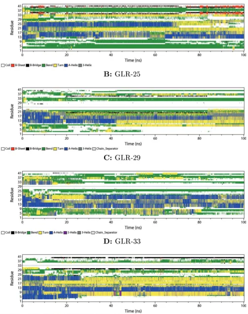
Figure 2: DSSP plots of Aβ42 simulated in 100% Water for 100 ns
The secondary structure assignment of the closed shell peptide (Figure 2A) shows bends in the region of the N-terminus (residues 1-10) during the whole simulation. In the middle region of the peptide (residues 11-27),α-helices are present. In the region of the C-terminus, bends,β-bridges,
andβ-sheets are forming. The β-bridges appear between Met-35 and Val-40, as well as between Leu-34 and Ile-41. The β-sheets appear at the same positions as the β-bridges do, when both β-bridges are present at the same time.
In Figure 2B the DSSP plot of Aβ GLR-25 is illustrated. During this simulation bends and turns are present in the area of the N-terminus (residues 1-10). The middle region (residues 11-23) formsα-helices and turns. After 20 ns there is aβ-bridge present between Phe-20 and Met-35. In the beginning of the simulation a short-livedβ-bridge was formed between Lys-28 and Val-40. At the C-terminus bends and turns are present.
Figure 2C displays the DSSP plot of the peptide with a radical at residue 29. At the N-terminus bends, turns and someα-helices are forming. The middle region (residues 11-23) formsα-helices and turns again (cf. Figure 2B). From 15-22 ns some very short-lived β-bridges form between Leu-17 and Ile-41. The same occurs from 19-27 ns between Ile-32 and Met-35.
The DSSP plot of the peptide with a radical at residue 33 is shown in Figure 2D. In the beginning of the simulationα-helices are present in the region of the N-terminus as well as in the middle region of the peptide. The helix at residues 11-15 is present for the entire duration of the simulation. The helices at the N-terminus and at residues 20-24 are disrupted after 25 ns, forming turns. At the C-terminus aβ-bridge is present after 12 ns. As the simulation proceeds this bridge is present more often.
A: Closed Shell
B: GLR-25
C: GLR-29
D: GLR-33
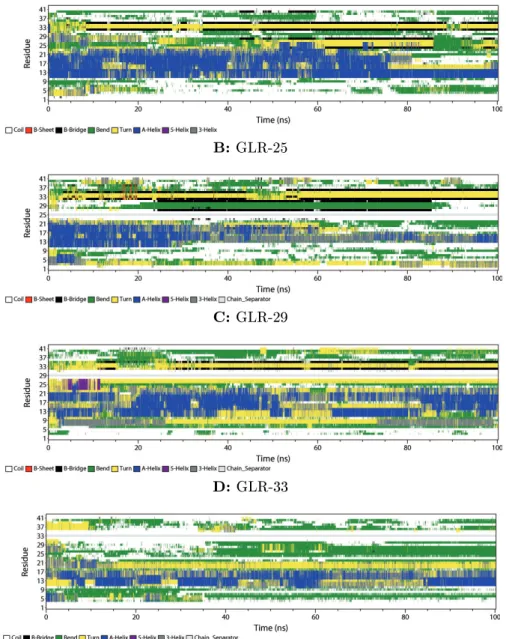
Figure 3: DSSP plots of Aβ42 simulated in 80% Water and 20% TFE for 100 ns
Figure 3 shows the DSSP plots of the four peptides that were simulated in a solvent containing 80% water and 20% TFE. Figure 3A displays the closed shell peptide. In the region of the N- terminus (residues 1-10) turns, bends, and coils form. The middle region (residues 11-23) forms mainlyα-helices. Some of them are disrupted during the simulation so that the helix gets shorter.
At 8 ns a β-bridge appears between Ile-32 and Met-35. Other β-bridges appear later in the simulation. For example, a brigde between Lys-28 and Val-40 is formed after 40 ns. Another β-bridge forms between Lys-28 and Val-24 after 60 ns of the simulation, which disrupts the bridge between Lys-28 and Val-40.
The DSSP plot of Aβ GLR-25 (Figure 3B) shows that bends and turns are formed at both termini. The middle region (residues 11-23) formsα-helices as it was observed for the closed-shell Aβ42. As the simulation proceeds a part of the helix is disrupted, which results in a helix present only at residues 13-19 at the end of the simulation. Aβ-bridge appears between Ile-32 and Met-35 after 3 ns of the simulation. A secondβ-bridge appears after 23 ns between Asn-27 and Ile-31.
This bridge lasts for 62 ns.
Figure 3C shows the DSSP plot of Aβ GLR-29. As it was already shown in the closed-shell Aβ 42 peptide, bends and turns are present at both termini, andα-helices are formed in the middle region of the peptide (residues 11-23). Aβ-bridge is forming between Ile-32 and Met-35.
The DSSP plot of the peptide with a radical at residue 33 (Figure 3D) also shows theα-helices in the middle region (residues 11-19). At the termini there are only coils and the rest of the peptide forms bends and turns without many characteristic secondary structures.
A: Closed Shell
B: GLR-25
C: GLR-29
D: GLR-33
Figure 4: DSSP plots of Aβ42 simulated in 20% Water and 80% TFE for 100 ns
In Figure 4 the DSSP plots of the simulations in 20% water are displayed. Figure 4A shows the plot of the closed-shell Aβ peptide. During this simulation anα-helix is located at the N-terminus, ending with a coil. After 75 ns the helix is disrupted, forming turns and bends. The middle region (residues 11-23) formsα-helices. In the beginning, there is aβ-bridge between Gly-33 and Met-35.
It appears for 6 ns. Afterwards the β-bridge is forming between Ile-32 and Val-36 that stays for 4 ns. After 15 ns of the simulation this bridge is reformed again, staying almost the whole time until the simulation ends. At 43 ns a secondβ-bridge is forming between Ser-26 and Ala-30.
In Figure 4B the DSSP plot of Aβ GLR-25 is illustrated. The middle region (residues 11-23)
formsα-helices again. Twoβ-bridges appear between Gly-33 and Val-36 after 5 ns, and between Glu-3 and Asp-7. The rst bridge is changing after 22 ns of the simulation. Then it is located between Leu-34 and Gly-37. After 27 ns of the simulationβ-sheets begin to form at both termini at the same positions were the bridges were found before. The β-sheets at the C-terminus are separated by a turn at Leu-34 and Met-35.
The DSSP plot of Aβ GLR-29 (Figure 4C) shows thatα-helices are formed at the N-terminus.
They reach from Asp-1 to Asp-23, disconnected by a turn at residues 8-10. During the simulation the helices are disrupted sometimes, but reformed very often. In the second half of the simulation someβ-bridges appear between Met-35 and Gly-38.
Figure 4D illustrates the DSSP plot of Aβ GLR-33. This plot looks similar to Figure 4C, but during this simulation more turns form, disrupting the helices. At the N-terminus an α-helix is formed after 33 ns. The C-terminus shows bends only. After 30 ns, one very short-livedβ-bridge is formed between Glu-22 and Ser-26.
4.2 Secondary Structure as a Function of Residue
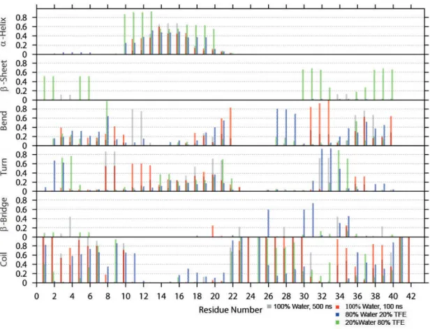
A dierent way to analyze the secondary structure is to plot the ratios of the time-averaged occurrence of α-helix, β-sheet, bend, turn, β-bridge and coil as a function of each residue. This secondary structure analysis is based on the DSSP outputs. The results are shown in Figures 5 - 8.
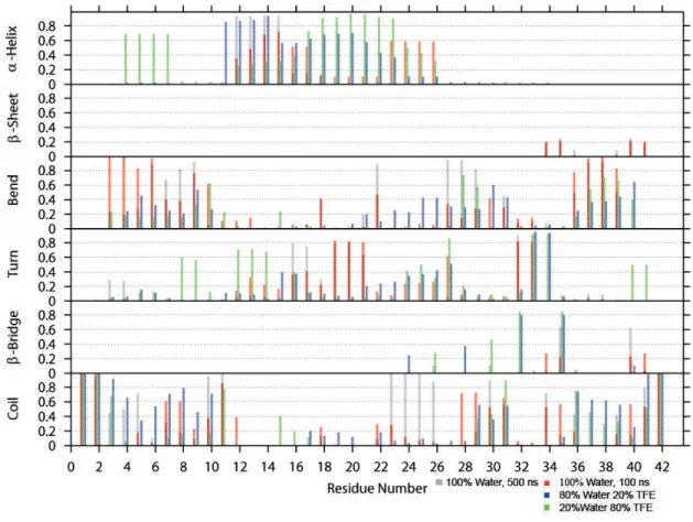
Figure 5: Time-averaged secondary structure as a function of residue for the closed-shell Aβ
Figure 5 illustrates the secondary structure analysis of the closed-shell Aβ42, simulated for 100 ns using the dierent solvent systems. In 100% water (Figure 5) one can see that anα-helix forms in the middle region of the peptide (residues 12-27), where β-sheets only appear close to the C-terminus. Bends form throughout Aβ CS, except from the helical region, but the bends are favored at the termini regions. Turns, however, appear mostly at residues 19-21 and 31-33. There areβ-bridges at the same positions as theβ-sheets, but the bridges appear more often during the simulation, indicating that the sheets (which involve at least two consecutive H-bonds) are not very stable. Both termini are without a certain secondary structure during the whole simulation, as only coils appear in these regions.
As the TFE concentration increases, theα-helices are shifted in the direction of the N-terminus.
But there are no moreβ-sheets forming any longer when TFE is present. Also the amount of bend decreases with TFE and the turn in the middle region disappears almost completely. However, closer to the termini the amount of turn is much higher in 20% water.
The 500 ns simulation of Aβ CS (Figure 5) is quite similar to the corresponding 100 ns simula- tion. There is more coil appearing in the middle region of the peptide (residues 23-26), but on the
other hand, the amount of theβ-bridge present between residues 35 and 40 is almost three times as high for the extended simulation. Theα-helix is shorter, as it only reaches from residues 12 to 15, but it is present almost the whole simulation. The next three residues sometimes form anα-helix, but they now favor a turn, as theα-helix decays.
Figure 6: Time-averaged secondary structure as a function of residue for Aβ GLR-25
Figure 6 illustrates the plot of AβGLR-25. TFE shows to have a great impact on the secondary structure of the peptide. With 20% TFE being present, compared to the closed-shell Aβ(Figure 5), more bends appear at residues 27-30, more turns appear at residues 31-34, and more β-bridges appear at residues 26, 30 and 31. The most interesting eect results during the simulation in 20% water (Figure 6). At both termini, β-sheets form with turns inbetween. The probability of the sheets being formed is up to 0.7. Just as theβ-sheets increase, theα-helix in the middle part is more likely, as well. Its amount increases up to 0.9, compared to 0.6 for the closed-shell Aβ (Figure 6).
During the 500 ns simulation of Aβ GLR-25 (Figure 6), Aβ is mostly unstructured.Turns are present at residues 7-21 most of the time, before anα-helix appears with a probability of up to 0.7.
Bends are favored at of the C-terminus. However, the C-terminus remains, except from residues 31 to 38, mostly unstructured. Residues 31 to 38 form transientβ-bridges andβ-sheets.
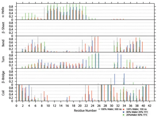
Figure 7: Time-averaged secondary structure as a function of residue for Aβ GLR-29
The analysis of Aβ GLR-29 (Figure 7) shows that the α-helix gets more stable as the con- centration of TFE increases. It occurs between residues 10 and 21. In 100% water bends form at residues 25 and 26. As the TFE concentration increases to 20%, these bends become turns, which is also indicative of the increased helical stability when TFE is present. Residues 31 and 34 form aβ-bridge, but only with 20% TFE being present. Other than that a lot of coils appear at the remaining residues. As for Aβ GLR-25, in neither solvent system β-sheets are formed. This combined with the reduced presence of β-bridges in Aβ GLR-25 and GLR-29 shows a reduced β-propensity compared to closed-shell Aβ.
Like for the 100 ns simulations of Aβ GLR-29 (Figure 7), anα-helix is present at residues 8-20, when this peptide is simulated in 100% water for 500 ns (Figure 7). Bends appear throughout the peptide without favoring a particular region, while turns are formed in the middle region, but they are closer to the N-terminus. Between residues Ala-30 and Leu-34 aβ-bridge is formed.
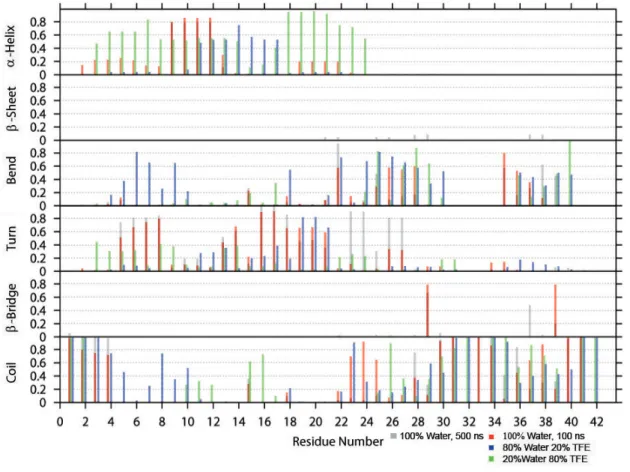
Figure 8: Time-averaged secondary structure as a function of residue for Aβ GLR-33
In Figure 8, illustrating the data of Aβ GLR-33, α-helices are present between residues 2 to 24. The helices appear in all three solvent systems. In 100% water the helix is mainly formed at residues 8-12, in 80% water theα-helix region shifts to residues 10-17, and nally, in 20% water, theα-helix is divided into smaller pieces and appear at residues 3-14, and 18-24. Bends appear throughout the peptide. But at residues 10-18 as well as at residues 31-35, the amount of bends is much lower than it is for the remaining residues. Turns, however, are more stable in 100% water.
Its appearance decreases as the TFE concentration increases, because the turns are replaced by proper helices. Next to that, coils only form at the termini.
The 500 ns simulation of Aβ GLR-33 in 100% water (Figure 8) does not reveal a very dierent behavior compared to the 100 ns simulation. They look very much alike with some probability dierences for theβ-bridges. After 100 ns the β-bridge appears with a probability of 0.8 between Gly-29 and Val-39, and after 500 ns the highest probability is 0.7 at Gly-29. Val-39 is even decreased to 0.2.
4.3 Radius of Gyration and RMSD
Figures 9 to 12 illustrate the analysis of the radius of gyration and the RMSD. One plot for each solvent system was generated. For both quantities, the population distribution is shown.
Figure 9: Plots of the radius of gyration (A) and the RMSD (B) of Aβ42 in 100% water simulated for 100 ns
In 100% water the closed-shell peptide has the smallest radius of gyration. The maximum of its curve in Figure 9A is at approximately 0.9 nm. All curves belonging to radicalized structures have their maximum at larger radii. 0.95 nm for GLR-33, 1.1 nm for GLR-29, and 1.0 nm for the GLR-25. The RMSD plot (Figure 9B) shows the same phenomenon. The closed shell peptide has the smallest RMSD (peak at 0.9 nm), which means that its structure stays the most similar to its starting structure. The radicalized structures appear to have an average RMSD value higher than 1.0 nm (GLR-33 at 1.1 nm, GLR-25 at 1.2 nm, GLR-29 at 1.4 nm).
Figure 10: Plots of the radius of gyration (A) and the RMSD (B) of Aβ42 in 80% water simulated for 100 ns
Figure 10A shows the radius of gyration of peptides simulated in 80% water. All curves have a fairly broad distribution. GLR-29 shows values from less than 1.0 nm to approx. 1.7 nm, and the closed-shell peptide reaches from 1.15 nm to 2.0 nm. Both curves of GLR-33 and GLR-25 span from around 1.0 nm to approx. 2.1 nm. The RMSD plot (Figure 10B) shows similar curves for the simulations. Their maxima are in the range of 0.7 - 1.0 nm and their distribution is within of each other. Only GLR-25 shows a very broad distribution.
Figure 11: Plots of the radius of gyration (A) and the RMSD (B) of Aβ42 in 20% water simulated for 100 ns
The data of the simulations in 20% water are shown in Figure 11. The radius of gyration of the radicalized peptide GLR-33 (Figure 11A) has two stable structures with quite dierent radii
(1.05 and 1.65 nm). The same appears for the corresponding RMSD in Figure 11B. The peptide GLR-33 forms two metastable structures, which appear as peaks in the RMSD plot. In Figure 11A, all radius of gyration curves, except for GLR-29, show two maxima. GLR-29 has its maximum at 1.5 nm, while the curves for GLR-25 and the closed-shell peptide have their maxima at the same positions, at approximately 1.2 nm and at 1.45 nm. The RMSD plot (Figure 11B) shows a broader distribution for GLR-25 than those of the other peptides. Their peaks are more dened.
The closed-shell and GLR-29 curves show their maxima at approximately 0.5 nm, while GLR-33 has a peak at 0.6 nm and its maximum can be found at approximately 1.3 nm.
Figure 12: Plots of the radius of gyration (A) and the RMSD (B) of Aβ42 in 100% water simulated for 500 ns
The 500 ns simulations of the dierent Aβ42 peptides in water are illustrated in Figure 12.
The analysis of the radius of gyration shows that GLR-33 has the smallest radius of gyration (Fig- ure 12A). The maximum of this curve is at approximately 0.88 nm. The other radii are of similar amplitudes. The GLR-25 has the highest population at approximately 0.95 nm, while the CS and the GLR-29 have a broader radius of gyration distribution. The RMSD plot (Figure 12B) shows that the maxima of the four graphs dier quite a lot. Where the closed-shell peptide has its maximum at 1.0 nm, the maxima of the radicalized peptides are between 1.2 nm (GLR-33) and 1.5 nm (GLR-25).
Compared to the 100 ns simulations, the radius of gyration of GLR-33 after 500 ns stays almost the same. But the data of all other Aβ peptides is shifted to higher values. The same occurs for the RMSD, with the dierence that in this case all curves are shifted to higher values.
4.4 Cluster Analysis
A very visual way to analyze MD simulations is the cluster analysis. This methods oers the possibility of taking a snapshot of representative structures of the simulation. Table 2 provides information about how many clusters have been found in total and the population of the largest clusters. The frames represent the time steps from when the pictures of the Figures 13 and 14 were taken.
Table2:Ratioofthelargestclustersinallsimulations PeptideSolventSimulationdurationNumberofclustersFrameofrepresentativestructureoflargestclusters[ns] andpercentofstructuresinthelargestcluster[%] Aβ42ClosedShell 100%Water100ns11234.2(84.9%) Aβ42GLR-25107067.8(57.9%) Aβ42GLR-2979460.7(14.7%) Aβ42GLR-33161058.2(61.9%) Aβ42ClosedShell 100%Water500ns461224.6(21.6%) Aβ42GLR-25872375.5(14.6%) Aβ42GLR-291474359.9(6.5%) Aβ42GLR-33160411.5(23.3%) Aβ42ClosedShell 80%Water20%TFE100ns129192.6(6.7%) Aβ42GLR-25277197.6(5.0%) Aβ42GLR-2998767.6(13.5%) Aβ42GLR-33239576.1(13.2%) Aβ42ClosedShell 20%Water80%TFE100ns7863.1(55.2%) Aβ42GLR-2514755.4(73.1%) Aβ42GLR-296360.6(26.6%) Aβ42GLR-3322877.5(35.8%)
Figure 13: Largest clusters of the 100 ns simulations.
Figure 13 shows the central structure from the largest cluster of all simulations that ran for 100 ns. The peptides are displayed with the N-terminus at the top. At the rst sight all peptides look quite helical. Especially the clusters of the simulations in 100% water show a helix in the same position that diers in length. The helix of the Aβ GLR-29 peptide is the longest one. The others are comparable in length. The radicals are relatively far from the C-terminal end of the helix.
The representative structures of the clusters of the simulations done in the solvent system with 80% water are less helical than the one in 100% water. Helices are present, but they are devided into smaller fragments (GLR-25 and GLR-29) or just much shorter (CS and GLR-33).
In 20% water all representative structures show at least one helix. They are more helical than the structures in 100% water. The cluster of GLR-25 is the only one showingβ-sheets at both termini. The β-sheets are in anti-parallel orientation. The radical is between the helix and the β-sheets at the C-terminus. The other three structures show two helices each. The closed-shell structure and the structure of Aβ GLR-29 have both a helix in the region of the N-terminus and one in the middle region. The radical in GLR-29 is at the C-terminal end of the helix. Compared to the closed-shell peptide, that has a helix at residue 29, the radical disrupts the helix during the simulation. Aβ GLR-33 shows two helices, but they are shorter in length. This structure looks more like the ones in 80% water.
Figure 14: Largest clusters of the 100 ns and the 500 ns simulations in 100% Water.
The 100 ns-MD simulation in 100% water was extended to 500 ns to analyze the changes that appear over a longer simulation interval. The comparison of the central structure of the largest cluster (Figure 14) show the changes quite well. The structure of GLR-29 does not change that much over time, except that the helix moves closer to the N-terminus after 100 ns. However the end of the helix does not change its distance from the radical.
All other clusters form anti-parallelβ-sheets in the region of the C-terminus. It is worth noting that the radical at residue 33 (GLR-33) is right at the end of the rst β-strand. The radical is located between the twoβ-strands, forming theβ-sheets. All structures show also helices.
5 Discussion
5.1 Secondary Structure
The DSSP analysis of the simulations in 100% water over 100 ns (Figure 2) generally contain, less secondary structure in the presence of a radical than in the closed-shell Aβ. Where the closed-shell Aβ peptide formsβ-sheets at the C-terminus, only Aβ with a radical at residue 33 forms a stable β-bridge at a similar position (cf. Figure 2A and D). The radical is located in the turn between the bridge. This might indicate that this radical stabilizes the formation ofβ-sheets in the end.
The dierent radicals have also dierent inuence on theα-helix in the middle region. Where GLR-25 and GLR-33 disrupt the helix almost entirely, GLR-29 stabilizes it. During the simulation of Aβ GLR-29 the region where α-helices appear, grows longer. However, residue 29 is not part of the helix. The time-averaged secondary structure plots as a function of residue (Figures 5 to 8) show similar results. If a radical appears to be in the peptide, there is less secondary structure.
Only for the closed-shell Aβ and the Aβ GLR-29 similar results are obtained.
If the solvent system consisting of 80% water and 20% TFE (Figure 3) is examined one can recognize that this shows similar trends as shown in Figure 2. The helix in the middle region is partly disrupted by the presence of GLR-33. β-bridges are present more often for GLR-25 and GLR-29 (cf. Figure 3 B and C). But dierent from GLR-33 in 100% water, the bridges are not formed around the radicals. Theβ-bridges between Ile-32 and Met-35 appear in all simulations.
Figure 3B (Aβ GLR-25) shows the formation of anotherβ-bridge between Asn-27 and Ile-31 that seems to be stabilized by the radical.
The solvent system of 20% water and 80% TFE (Figure 4) favors the formation ofα-helices.
Only the radical at residue 25 favors the formation of β-sheets, which appear at both termini.
Where all peptides with 20% TFE present form many bends, turns and coils, the four simulations displayed in Figure 4 (Aβ simulated in 80% TFE) favorα-helices andβ-sheets, even though bends, turns, and coils are still present in these peptides, too. The fact thatα-helices are favored during these simulations might be due to 80% TFE being present, because TFE tends to stabilizeα-helices [26].
However, the inuence of TFE on Aβ is not easily understood. 20% TFE being present has a helix-destabilizing inuence, referring to the DSSP analysis, but 80% TFE seems to stabilize, or maybe even over stabilizeα-helices. Evidence of TFE being an important factor to stabilize the structures can be seen in Figures 7 and 8. As TFE increases to 80%, the probability of theα-helix increases as well. Moreover theβ-turns at residues 20-26 are also stabilized by TFE, as shown in Figure 7. The same appears for theβ-bridge between residues Ile-31 and Leu-34, displayed in the
same gure.
5.2 Radius of Gyration and RMSD
The radius of gyration and RMSD analysis conrmed that radicals induce conformational changes in the Aβ42 peptide. Figures 9A and B correlate with each other. Where the radius of gyration decreases, the RMSD increases. The maxima of the curves follow the same order. Aβ CS has the smallest radius of gyration and the smallest RMSD, followed by Aβ GLR-33, Aβ GLR-25, and Aβ GLR-29.
The 500 ns simulation is illustrated by Figure 12A. At rst sight it looks like the radii change a lot compared to the radius of gyration of Aβ CS after 100 ns, but what really happens is that the distribution becomes more narrow. The overall range decreases from 0.8-1.9 nm to 0.8-1.2 nm.
At the same time the populations increase over time which means that structures that have this radius of gyration, appear more often during the simulation. The RMSD analysis, Figure 12B, shows that all curves are shifted to higher values as the simulation proceeds. The gap between the maxima increases as well with more sampling time, and the radicalized Aβ peptides dier much more from the starting structure than the closed shell peptide does. This fact denitely shows the inuence of the radical on the conformation of Aβ.
As the cluster analysis already showed (Figure 13) the Aβ peptide moves a lot in 80% water.
The same is illustrated in Figure 10A. The uctuation of the radius of gyration is very high. The RMSD plot (Figure 10B) also illustrates the constant movement of the peptide by the fairly broad distribution of the curves.
The radius of gyration plot of the simulations in 20% water correlates with the RMSD plot of the same simulations. Especially the two clusters of Aβ GLR-33 can be assigned to each other.
The radius of gyration peak at 1.05 nm corresponds to the RMSD peak at 1.3 nm, so does the wide 1.6 nm radius of gyration peak with the distributed 0.6 nm RMSD peak. The RMSD values are, except for the higher peak of GLR-33, clearly lower for these simulations. The TFE stabilizes the helices, so that Aβ moves less than before. They are less exible than the peptides that were simulated in 100% water. This especially refers to Aβ GLR-25 and Aβ GLR-29.
5.3 Cluster Analysis
The cluster analysis of the simulations shows the inuence of the radicals on other residues, yielding in conformational changes. For example, the inuence of the radical can be observed in the illustration of the Aβ GLR-29 (Figure 13) simulated in 20% water. The position of the radical is at the end of the helix. Since the closed shell peptide forms anα-helix at this position (Figure 5) it is likely that the radical is the reason why this helix is disrupted.
The overall picture shows that there is no linear connection between the secondary structure stability and TFE being present. If little TFE (20%) is added the amount of secondary structure decreases (c.f. Figures 2 and 3). This fact is also visualized by Figure 13. If more TFE (80%) is added the amount of secondary structure increases drastically. This is conrmed by Figures 3 and 4, as well as Figure 13.
The 500 ns simulations show another interesting element. The DSSP analysis showed that there is only very littleβ-sheet formation taking place (Figures 5, 6, 7, 8), but the cluster analysis showed that the largest clusters of the closed shell peptide and the radicalized peptides GLR-25 and GLR-33 (Figure 14) appear to haveβ-sheets, anyhow. A possible explanation is the cuto used to compute the clusters. Since the three peptides showβ-bridge structures at the same positions where theβ-sheet appears, the program probably counted the present β-bridges as β-sheets, due to the cuto. This means that the structures of theβ-bridges are very much alike to theβ-sheets.
Therefore the cluster analysis shows clusters withβ-sheets, even though most of the simulation time there are onlyβ-bridges present. Another possible reason is that the visualization program VMD uses a dierent program to calculate the secondary structure than the DSSP program does.
Therefore it is possible that the VMD program interprets the structures dierently and assignes β-sheets, where the DSSP program assignesβ-bridges.
Table 2 lists the proportions of the total structures in largest clusters. Eye-catching are the values of the simulation that were done in 80% water and 20% TFE. The program found at least 987 clusters, which is a relatively high number. Therefore the ratios of the largest clusters are between 5.03% and 13.59%. These values appear because the peptides move a lot during the simulations. The same conclusion can be drawn from the radius of gyration analysis shown in Figure 10A. The uctuation is obvious here as well. All in all, one can say that the clusters of these simulations are not well representative due to the constant conformational changes.
6 Conclusion and Prospects
In an attempt to attain a better understanding of AD, several hypotheses about the causes of this neurological disorder exist. One of them is the relationship between aggregation of Aβ and oxidative stress, primary due to dierent radicals, such as the hydroxyl radical. Radicals appear in every metabolism, and as long as there are enough reductive species present, radicals do not appear to be dangerous. But if an imbalance occurs, radicals can cause severe damage to cells. If a radical and an Aβ peptide react, the abstraction of an H• from a glycine residue is one of the favored reactions due to steric reasons. Aβ oers glycine residues in six dierent positions. For this work residues 25, 29, and 33 were examined. To simulate Aβ in more realistic surroundings dierent water/uorinated alcohol solvent systems were used and compared to simulations done in water only.
The DSSP analysis of the simulations was a rst step to get an overview of the secondary structures elements that are present at dierent positions of the Aβpeptides during the simulation.
Converting these plots to time-averaged secondary structure analysis dependent on the residue made it easier to examine the frequencies of the structural elements appearing at a certain residue.
This way of displaying the obtained data helped comparing the eects of TFE on the secondary structure.
Even though TFE has an eect on secondary structure there is no real pattern to it. The addition of 20% TFE did not show a stabilizing impact on the secondary structure. It was the other way around. In 20% TFE the α-helices and β-sheets present in the peptide disappeared, forming bends, turns and coils. The peptide was very exible and moving a lot, without forming representative clusters. On the other hand, in 80% TFE the secondary structure was stabilized and Aβ GLR-25 even formed very stable β-sheets that stayed throughout the whole simulation duration. The idea of the 500 ns simulations was to consider the simulation time being a factor on the conformation of Aβ as well. This time, TFE as a variable was dismissed to identify if the eect it has on Aβ GLR-25 in 20% water, is a eect that occurs in water as well with more sampling time. So the simulations in water were extended for 400 ns, yielding 500 ns simulations. With more sampling time more β-sheets were present, but it was still much less than the amount of β-sheets present in 20% water.
One way to keep studying the eect is to extend the simulations in water even more. An alternative is the use of replica exchange-MD simulations (REMD). Using this method, multiple simulations run simultaneously at dierent temperatures to be able to cross energy barriers more easily at higher temperature while obtaining the correct canonical distribution at the temperature of interest.
Further, the RMSD analysis showed that TFE inhibits large-scale motions in Aβ. Aβ is less exible and changes less compared to the starting structure, which is conrmed by the RMSD values. The more TFE was present as a co-solvent, the smaller the RMSD values were compared to the simulations in 100% water.
The simulations of Aβ42 showed that the radicalized structures of the peptide behave quite dierent from the closed-shell peptide. Especially the radius of gyration analysis revealed this.
The closed-shell peptide is very compact, whereas the structures of the radicalized Aβ peptides are loosened up. In most cases, their radii of gyration are clearly greater than it is for the closed-shell Aβ. Therefore it is obvious that there is an eect of radicals on the conformation of Aβ42. The radicals appear to stabilize secondary structure elements, especiallyβ-bridges and eventually even β-sheets.
All in all, one has to be careful by interpreting the results of MD simulations with Aβ. Because Aβ is very hard to handle in the laboratory, due to its aggregation behavior, there are not many representative experimental results. A question that follows from the results is if longer simulations (i.e. better sampling) show even stronger evidence of β-sheets being stabilized by radicals. In addition to that one could explore the eects of other residues being radicalized. Possible residues are the other three glycine residues at positions 9, 37, and 38 which could be compared to the results from this work. Finally, a prospect of further work could be the studying of the eect of glycine radicals on the aggregation on the Aβ peptide. Since the aggregation is likely the reason that leads to the neuronal cell death in AD, it is more important to see if the glycine radicals can induce the aggregation or if they can accelerate the process. The understanding of it is an important step in the understanding of Alzheimer's disease.
7 Appendix References
[1] Boutajangout, A.; Wisniewski, T. Tau-Based Therapeutic Approaches for Alzheimer's Disease - A Mini-Review. Gerontology. 2014
[2] Alzheimer's Disease International, World Alzheimer Report 2010 - The Global economic impact of dementia [http://www.alz.co.uk/reseach/les/WorldAlzheimerReport2010.pdf]
[28.08.2014]
[3] Alzheimer's Association, Gehirn-Tour, Chicago, 2008 [http://www.alz.org/de/gehirn- deutsch.asp#deutsch] [04.09.2014]
[4] Hernandez-Rodriguez, M. et. al. Design of Multi-Target Compounds as AChE, BACE1, and Amyloid-β (1-42) Oligomerization Inhibitors: In Silico and In Vitro Studies. Journal of Alzheimer's Disease. April 24, 2014, Vol. 41
[5] Brown, L.A.M.; Jin, J.; Ferrel D.; Sadic E.; Obregon D. et al. Efavirenz Promotesβ-Secretase Expression and Increased Aβ1-40, 42 via Oxidative Stress and Reduced Microglial Phagocy- tosis: Implications for HIV Associated Neurocognitive Disorders (HAND). Plos One. April 23, 2014
[6] Swomley, A. M. et al. Abeta, oxidative stress in Alzheimer disease: Evidence based on pro- teomics studies. Biochimica et Biophysica Acta 1842. 2014, pp. 1248-1257
[7] R&D systems, Minireviews - Reactive Oxygen Species (ROS), Minneapolis, 1997 [http://www.rndsystems.com/mini_review_detail_objectname_MR97_ROS.aspx]
[7.10.2014]
[8] Cuajungco, M. P. et al. Evidence that theβ-Amyloid Plaques of Alzheimer's Disease Represent the Redox-silencing and Entombment of Aβ by Zinc. J. Biol. Chem., 2000, Vol.275, pp.
19439-19442
[9] Viehe, H. G.; Janousek Z.; Merenyi R.; Stella L. The Captodative Eect. Acc. Chem. Res.
1985, Vol. 18, pp. 148-154
[10] Rauk, A.; Armstrong, D.A. Inuence ofβ-Sheet Structure on the Susceptibility of Proteins to Backbone Oxidative Damage: Preference for α-C-centered Radical Formation at Glycine Residues of Antiparallelβ-Sheets. J.Am.Chem. Soc., 2000, Vol. 122, pp. 4185-4192
[11] Rauk, A.; Armstrong, D.A.; Fairlie, D. P. Is Oxidative Damage by β-Amyloid and Prion Peptides Mediated by Hydrogen Atom Transfer from Glycineα-Carbon to Methionine Sulfur withinβ-Sheets? J. Am. Chem. Soc. 2000, Vol. 122, No. 40, pp. 9761-9767
[12] Lexikon-Intitut. Bertelsmann-das neue Universal Lexikon. wissenmedia Verlag, Gütersloh, München, 2006
[13] Buck, M. Triuoroethanol and colleagues: cosolvents come of age. Recent studies with peptides and proteins. Quarterly Reviews of Biophysics, 1998, Vol. 31, pp. 297-355
[14] Fiorini, M.; Diaz, M.D.; Burger, K.; Berger, S. Solvation Phenomena of a Tetrapeptide in Wa- ter/Triuoroethanol and Water/Ethanol Mixtures: A Diusion NMR, Intermolecular NOE, and Molecular Dynamics Study. J. Am. Chem. Soc. 2002, Vol. 124, pp. 7737-7744
[15] Angulo, M.; Berger, S. The pH dependence of the hydrophobic eect of triuorethanol. Ana- lytical and Bioanalytical Chemistry, 2004, Vol. 378, pp. 1555-1560
[16] Frenkel, D.; Smit, B. Understanding Molecular Simulation: From Algorithms to Applications (Computational Science). Academic Press, Bodmin-Cornwall, 2002
[17] Kaminski, G.A.; Friesner, R:A. Evaluation and Reparametrization of the OPLS-AA Force Field for Proteins via Comparison with Accurate Quantum Chemical Calculations on Peptides.
J. Phys. Chem. B. 2001, Vol. 105, pp. 6474-6487
[18] Jorgensen W.L., Maxwell D.S., Tirado-Rives J. Development and Testing of the OPLS All- Atom Force Field on Conformational Energetics and Properties of Organic Liquids. J. Am.
Chem. Soc. 1996, Vol. 118, pp.1122511236
[19] Pronk, et al. GROMACS 4.5: a highly parallel open source molecular simulation toolkit.
Bioinformatics 2013, Vol. 29, pp.845-854
[20] Komáromi, I.; Owen, M.C.; Murphy, R.F.; Lovas, S.J. Development of glycyl radical parame- ters for the OPLS-AA/L force eld. Comput. Chem. 2008, Vol. 97, pp. 1999-2009
[21] Berendsen, H.J.C. et al. Molecular dynamics with coupling to an external bath. J. Chem.
Phys., 1984, Vol. 81, pp. 3684.
[22] Parrinello, M.; Rahman, A. Polymorphic transitions in single crystals: A new molecular dynamics method. J. Appl. Phys., 1981, Vol. 52, pp. 7182.
[23] Kabsch, W.; Sander C. Dictonary of Protein Secondary Structure: Pattern Recognition of Hydrogen-Bonded and Geometrical Features. Biopolymers 1983, Vol. 22, pp. 2577-2637
[24] Baldwin R. L. In Search of the Energetic Role of Peptide Hydrogen Bonds. J. Biol. Chem.
2003, Vol.278, pp. 17581-17588
[25] Daura, X., et al. Peptide folding: when simulation meets experiment. Angew. Chem. Int. Ed., 1999, Vol. 38, pp. 236240
[26] Rajan, R.; Balaram, P. A model for the interaction of triuorethanol with peptides and proteins. Int. J. Peptide Protein Res. 1996, Vol. 48, pp. 328-336
List of Figures
1 Illustration of Aβ42 (pdb-code: 1Z0Q) The Figure was generated by the program Visual Molecular Dynamics (VMD). The representation was done with the New Cartoon drawing method. The coloring method was Secondary Structure. The N- terminus and the C-terminus are representend by the red and blue beads, respectively. 3 2 DSSP plots of Aβ42 simulated in 100% Water for 100 ns . . . 13 3 DSSP plots of Aβ42 simulated in 80% Water and 20% TFE for 100 ns . . . 15 4 DSSP plots of Aβ42 simulated in 20% Water and 80% TFE for 100 ns . . . 17 5 Time-averaged secondary structure as a function of residue for the closed-shell Aβ 19 6 Time-averaged secondary structure as a function of residue for Aβ GLR-25 . . . . 20 7 Time-averaged secondary structure as a function of residue for Aβ GLR-29 . . . . 21 8 Time-averaged secondary structure as a function of residue for Aβ GLR-33 . . . . 22 9 Plots of the radius of gyration (A) and the RMSD (B) of Aβ42 in 100% water
simulated for 100 ns . . . 23 10 Plots of the radius of gyration (A) and the RMSD (B) of Aβ42 in 80% water simu-
lated for 100 ns . . . 24 11 Plots of the radius of gyration (A) and the RMSD (B) of Aβ42 in 20% water simu-
lated for 100 ns . . . 24 12 Plots of the radius of gyration (A) and the RMSD (B) of Aβ42 in 100% water
simulated for 500 ns . . . 25 13 Largest clusters of the 100 ns simulations. . . 28 14 Largest clusters of the 100 ns and the 500 ns simulations in 100% Water. . . 30
List of Tables
1 MD Simulations that were performed for 100 ns . . . 9 2 Ratio of the largest clusters in all simulations . . . 27


![Spectroelectrochemical investigations of the complexes showed the formation of a [(R- PyMA)Ni(Aryl)(Solv)]](data:image/gif;base64,R0lGODlhAQABAIAAAP///wAAACH5BAEAAAAALAAAAAABAAEAAAICRAEAOw==)