Agency Costs and the Monetary Transmission Mechanism

IHS Economics Series Working Paper 328

March 2017

Agency Costs and the Monetary Transmission Mechanism

Michael Reiter

Tommy Sveen

Lutz Weinke

Impressum Author(s):

Michael Reiter, Tommy Sveen, Lutz Weinke Title:

Agency Costs and the Monetary Transmission Mechanism ISSN: 1605-7996

2017 Institut für Höhere Studien - Institute for Advanced Studies (IHS) Josefstädter Straße 39, A-1080 Wien

E-Mail: o ce@ihs.ac.atffi Web: ww w .ihs.ac. a t

All IHS Working Papers are available online: http://irihs. ihs. ac.at/view/ihs_series/

This paper is available for download without charge at:

https://irihs.ihs.ac.at/id/eprint/4219/

Agency Costs and the Monetary Transmission Mechanism

Michael Reiter

^a

, Tommy Sveen

^b

, Lutz Weinke

^c

aInstitute for Advanced Studies, Vienna bBI Norwegian Business School cHumboldt-Universität zu Berlin

February 13, 2017

Abstract

Once New Keynesian (NK) theory (see, e.g., Woodford 2003) is combined with a standard model of investment (see, e.g., Thomas 2002), the result- ing framework loses its ability to generate a realistic monetary transmission mechanism. This is the puzzle uncovered in Reiter et al. (2013). The simple economic reason behind it is the unrealistically large interest rate elasticity of investment, as implied by standard investment theory. In order to address this puzzle we develop a NK model featuring fully ‡exible investment combined with a …nancial friction in the spirit of Carlstrom and Fuerst (1997). This model is used to isolate the quantitative importance of the …nancial friction for the monetary transmission mechanism.

Keywords: Financial Frictions, Sticky Prices.

JEL Classi…cation: E22, E31, E32

1 Introduction

What explains the short-run e¤ects of monetary policy on real variables of inter- est? Over the past twenty years dynamic stochastic general equilibrium (DSGE) models featuring nominal rigidities, such as sticky prices or wages combined with monopolistic competition, have emerged as the standard tool to analyze questions related to the dynamic consequences of monetary policy changes. Those models are generally called New Keynesian (NK) theory. Its micro-founded structure makes this theory in principle usable for policy analysis and, in fact, NK theory is being used in the academic world as well as in central banks and other policy institutions to understand a wide range of issues related to monetary policy. However, the nor- mative results of NK theory are only useful if its positive predictions are relevant from an empirical point of view. The monetary transmission mechanism is therefore generally viewed as being the hallmark of NK theory (see, e.g., Woodford 2003, p.

6, and Galí 2015, p. 1).

It is well understood by now that smoothness in aggregate capital accumulation is necessary to obtain a reasonable monetary transmission mechanism in the context of NK models.

¹

This has motivated Christiano et al. (2005) and Woodford (2005) to introduce adjustment costs into the investment block of the NK framework, and most of the related literature has followed their lead.

²

But the existence of those adjustment costs makes NK models inconsistent with the observed lumpiness in plant-level investment.

³

Motivated by this problem our work in Reiter et al. (2013) uses standard investment theory (see, e.g., Thomas 2002) to make an otherwise con- ventional NK DSGE model consistent with the lumpy nature of capital adjustment at the micro level. In the context of the resulting framework the following puzzle emerges. Monetary shocks are shown to have dynamic consequences whose strength and persistence are out of line with the data. Speci…cally, the impact responses of investment and output to a change in the nominal interest rate become very large and the dynamic consequences of that shock are only short-lived.

⁴

In a nutshell, the

1It is therefore even common in the NK literature to abstract from capital accumulation (see, e.g., Galí 2015, among many others).

2Speci…cally, Christiano et al. (2005) assume a convex investment adjustment cost, whereas Woodford (2005) postulates a convex capital adjustment cost.

3That lumpiness is reported by, e.g., Doms and Dunne (1998), Thomas (2002) and Khan and Thomas (2008). In the context of our theory there is no distinction between a plant and a …rm and we therefore use those terms interchangeably.

4Given the large size of the literature on the monetary transmision mechanism of might wonder why the puzzle presented in Reiter et al. (2013) has not been uncovered before. The simple reason is that the general equilibrium consequences of multiple (S,s) decisions at the micro level can not easily be computed. In Reiter et al. (2013) we have relied on the method developed in Reiter (2009, 2010) to bring this about.

reason behind the main result in Reiter et al. (2013) is that non-convex adjustment costs which are routinely assumed in the investment literature do not rationalize a realistic interest rate sensitivity of investment. The (S,s) nature of investment deci- sions is crucial to understand this result. In response to an expansionary monetary policy shock …rms choose to undertake some of the investment activity that they would have otherwise done later. This mechanism, which is often called an extensive margin e¤ect (see, e.g., Caballero and Engel 2007), explains the unrealistically large interest rate elasticity of investment in Reiter et al. (2013).

The motivation for the present paper originates in this puzzle. In fact, we assess the quantitative importance of a simple economic mechanism to address it. More concretely, Carlstrom and Fuerst (1997) show that a …nancial friction in the process of capital production might act as a smoothing device. In order to isolate the role of this mechanism we formulate a NK model featuring otherwise fully ‡exible investment combined with a …nancial friction in their spirit.

⁵

That friction can, in principle, perfectly coexist with lumpiness in plant-level investment. This is important because many other frictions make the model inconsistent with lumpy investment, once they have a size that gives rise to a realistic monetary transmission mechanism.

⁶

It is therefore interesting that a plausible calibration of the …nancial friction under consideration makes our model go a long way towards an empirically relevant monetary transmission mechanism.

The remainder of the paper is organized as follows. Section 2 outlines the model.

Section 3 presents the dynamic analysis and section 4 concludes.

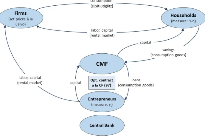
2 The Model

Our model integrates a …nancial friction in the spirit of Carlstrom and Fuerst (1997) into an otherwise standard New Keynesian model of the monetary transmission mechanism. Fig.

1

summarizes the model structure.

[Figure

1

about here.]

Since the details of the model features have been discussed elsewhere (see, Carl- strom and Fuerst 1997 for a discussion of the …nancial friction and, e.g., Woodford 2003 or Galí 2015 for textbook treatments of the New Keynesian elements) we turn

5Carlstrom and Fuerst (2001) also propose a monetray version of their (1997) RBC model. But this involves a cash-in-advance constraint, whereas we consider a standard cashless NK economy.

6For instance, Reiter at al. (2013) show that a convex capital adjustment cost at the …rm level combined with a (S,s) restriction on investment gives rise to a realistic monetary transmission mechanism only to the extent that the size of the convex cost is large enough to eliminate a plausible degree of lumpiness in investment.

directly to the implied set of equilibrium conditions. There is a continuum of …rms and each of them is the monopolistically competitive producer of a di¤erentiated good. Firms hire labor, rent capital from households and entrepreneurs and set prices in a staggered fashion à la Calvo (1983). Each …rm has access to the follow- ing production function using capital, households’labor and entrepreneurial labor as inputs

Y_t=F(K_t;(1 )L_t; );

(1)

where

Y_t

is output of its di¤erentiated consumption good. Our notation re‡ects the assumptions that there is a measure

(1 )

of households and a measure of entrepreneurs. Moreover households’ labor supply,

L_t

, is elastic, whereas each entrepreneur supplies inelastically one unit of labor. The capital stock used in time

t

production is denoted by

K_t

.

Cost minimization on the part of …rms implies the following set of factor prices

r_t = F_K(K_t;(1 )L_t; )

M_t ;

(2)

w_t = F_H(K_t;(1 )L_t; )

M_t ;

(3)

x_t = F_He(K_t;(1 )L_t; )

M_t ;

(4)

where

r_t

,

w_t

and

x_t

denote, respectively, the real rental rate for capital, the real wage and the real wage for entrepreneurial labor. They are given by the associated marginal products combined with the average price markup,

M_t

.

Households’labor supply equation reads

=w_tU⁰(C_t);

(5)

where is a parameter, re‡ecting our assumption of a linear disutiliy associated with supplying labor. As usual,

U⁰(C_t)

indicates the marginal utility of consumption and

C_t

is the households’ time

t

consumption level of a Dixit-Stiglitz aggregate.

Households decide how much of their labor and capital income to consume in the

same period, and how much to save by investing in capital accumulation. If a

household wishes to purchase capital, it must fund entrepreneurial projects, and

these projects are subject to agency problems. As in Carlstrom and Fuerst (1997),

households arrange their lending through a capital mutual fund (CMF). For each

unit of investment that a household wishes to purchase, it gives

q_t

consumption

goods to the CMF. The additional capital resulting from time

t

investment becomes

productive with a one-period delay and the Euler equation characterizing the optimal

consumption/savings decision therefore takes the following standard form

q_tU⁰(C_t) = E_tn

U⁰(C_t+1) [q_t+1(1 ) +r_t+1]o

;

(6)

where parameter is the discount factor for utility and parameter is the rate of depreciation.

The CMF uses the resources obtained from households to provide loans to an in…nite number of risk-neutral entrepreneurs. Entrepreneurs get access to the ag- gregate consumption good through the CMF in exchange for the promise to repay with interest in terms of the capital good they produce. More concretely, an entre- preneur with net worth

n

who borrows

(i n)

consumption goods agrees to repay

1 +r^k (i n)

capital goods to the lender. Entrepreneurs place their entire net worth as well as the borrowed consumption goods into their capital-creation tech- nology. The latter is assumed to be stochastic. It contemporaneously transforms

i

consumption goods into

!i

units of capital. The random variable

!

is i.i.d. across time and entrepreneurs. Agency issues emerge by assuming that

!

is privately ob- served by the entrepreneur. Others can observe

!

only at a monitoring cost of

i

units of capital. This information asymmetry creates a moral hazard problem be- cause, without monitoring, the entrepreneur might not wish to tell the true value of

!. However, the contract considered in Carlstrom and Fuerst (1997) incentivizes

entrepreneurs to always truthfully report the

!

realization. This contract takes a simple form. If an entrepreneur reneges on the promise to repay the speci…ed quan- tity of capital goods, monitoring occurs with probability one.

⁷

Entrepreneurs also work for …rms and generate an associated labor income which prevents them from having a zero level of net worth. A related point is that entrepreneurs do not accu- mulate net worth to the point that the agency problem disappears. In Carlstrom and Fuerst (1997) that is made sure by assuming that entrepreneurs discount the future more heavily than do households. In our context, this assumption would also guar- antee that the above mentioned contracting problem between entrepreneurs and the CMF is well-de…ned at each point in time. However, risk neutrality combined with an interior solution implies an in…nite intertemporal elasticity of substitution and thus gives rise to extreme ‡uctuations in entrepreneurial consumption and highly volatile investment dynamics in the equilibrium of our model. We will come back to this later. In order to avoid this problem, we adopt instead a classical assumption that has been popularized by Bernanke et al. (1999). Speci…cally, entrepreneurs are assumed to consume a constant fraction out of their net worth

n_t

. Entrepreneurial consumption,

C_e;t

, therefore takes the following form

7See Carlstrom and Fuerst (1997) for a discussion of the optimality of that contract.

C_e;t =c_en_t;

(7) with

c_e

denoting the fraction of net worth that entrepreneurs consume in the current period. To raise internal funds entrepreneurs supply labor and rent out capital to

…rms. They sell the remaining undepreciated capital to the CMF for consumption goods (the input used in their production technology). In the aggregate, entrepre- neurs’budget constraint takes the following form

nt=xt+ Z_t[q_t(1 ) +r_t]

;

(8)

where

Z_t

denotes the aggregate entrepreneurial capital stock. The latter evolves according to a law of motion of the form

Z_t = n_{t 1}roi_{t 1} q_{t 1}

C_{e;t 1}

q_{t 1} ;

(9)

with

roi_t

measuring an entrepreneur’s return on investment. The latter takes into account that net worth is leveraged into an investment project. Entrepreneurs keep a fraction of the resulting capital, and capital is priced at

q_t

. Carlstrom and Fuerst (1997) show that

roi_t

is determined by

roi_t = q_tf(!_t; )

1 q_tg(!_t; );

(10)

with function

f(!_t; )

measuring the fraction of the expected net capital output received by an entrepreneur. Its …rst argument is the critical value for idiosyncratic productivity,

!_t

: a project gets monitored, if an entrepreneur reports an idiosyn- cratic productivity level below that value. Its second argument is the standard deviation of the distribution of entrepreneurs’ idiosyncratic technology. Similarly, function

g(!_t; )

measures the fraction of the expected net capital output received by the CMF. The aggregate law of motion of the capital stock is of the form

K_t+1 = (1 )K_t+ I_t[1 (!_t; _d; ) ];

(11)

where the second term re‡ects the assumption that capital is produced by entre-

preneurs and part of that production is lost due to agency costs. As it turns out,

that loss depends on the (linear) monitoring cost , the distribution of entrepre-

neurs’s idiosyncratic technology (assumed to be normal with mean

_d

and standard

deviation ) as well as on the critical value for idiosyncratic productivity,

!_t

. Carl-

strom and Fuerst (1997) show how this critical value is obtained from two …rst-order

conditions implied by the agency problem. They read

q_t = 1

1 (!_t; _d; ) + (!_t; _d; ) _f^{f(!t; )}

!(!t; )

;

(12)

I_t = n_t

1 q_tg(!_t; ):

(13)

In stating the last two equations we have used the notation

(!_t; _d; )

for the density of entrepreneurs’idiosyncratic technology evaluated at the critical value

!_t

, and

f_!(!_t; )

is meant to indicate the derivative of function

f

with respect to its

…rst argument. The aggregate goods market clearing condition is of the form

Y_t= (1 )C_t+ C_e;t+ I_t:

(14)

As it is usual in the new Keynesian literature, gross in‡ation

t Pt

Pt 1

(with

P_t

denoting the time

t

price of the aggregate consumption good) is obtained from averaging optimal pricing decisions in a Calvo environment via the price index. The latter implies

t= _p+ (1 _p) (p_t)^{1 "}

1 1 "

;

(15)

with

p

denoting the Calvo parameter, i.e., the probability according to which a

…rm is not allowed to change price in a given period. Parameter

"

measures the elasticity of substitution between the di¤erentiated consumption goods in our econ- omy. Finally, we have used the notation

p_{t P}^Pt

t 1

for the optimal newly set price,

P_t

, that is chosen by all time

t

price-setters in our model, relative to the price of the consumption good one period earlier. The stochastic discount factor,

Q_t;t+1

, for nominal random pro…ts is of the form

Q_t;t+1 U⁰(C_t+1) U⁰(C_t)

P_t

P_t+1:

(16)

Let us also notice that up to a …rst-order approximation our model implies a standard inverse relationship between the real marginal cost,

^r_t

, and the average price markup

r

t = 1

M_t:

(17)

The …rst-order condition for price-setting takes the standard form for a constant returns technology (see, e.g., Galí 2015, p. 56)

X1

k=0

E_t Q_t;t+kY_t+kjt(1=P_t+k) P_t ^{p n}_t+k = 0;

(18)

with

ⁿ_t

indicating the time

t

nominal marginal cost, and

Y_t+kjt

denoting output in

period

t+k

for a …rm that last reset its price in period

t. Parameter ^p _"^"₁

is

the desired frictionless price markup. To close the model we assume a Taylor-type rule for the conduct of monetary policy

R_t= (R_{t 1}) ^r

"

t Y_t

Y

y#1 _r

e^er;t:

(19)

The shock,

e_r;t

, is

i:i:d:

with zero mean and monetary policy shocks are assumed to be the only source of aggregate uncertainty. Parameters and

_y

indicate the long-run responsiveness of the nominal interest rate to changes in current in‡ation and output,

⁸

respectively, and parameter

_r

measures interest rate smoothing.

3 The Monetary Transmission Mechanism

Our model will be used to quantify the e¤ects of a monetary policy shock. A baseline calibration of that model is presented next.

3.1 Baseline Calibration

The model period is a quarter. The discount factor, , is set to

0:99, which implies an

annualized steady state real interest rate of about

4

percent. Annualized steady state in‡ation is assumed to be two percent. As to the interest rate rule coe¢ cients, it is assumed

= 1:5; _y = 0:5=4

and

_r= 0:7. Moreover, the elasticity of substitution

between the di¤erentiated goods,

", is set to 7. We also assume p = 0:75

implying an average expected life-time of a price of

4

quarters. Those parameter values are consistent with the corresponding choices in Reiter et al. (2013). Other parameter values are justi…ed in Carlstrom and Fuerst (1997). In particular, the depreciation rate, , is set to

0:02. The production function is assumed to be of the Cobb-

Douglas form with capital-share parameter,

K = 0:36, labor-share, H = 0:6399,

and entrepreneurial labor-share,

He = 0:001. The fraction of entrepreneurs, , is set

to

0:003. Our baseline choice for the bankruptcy cost parameter, , is0:25, a value in

what Carlstrom and Fuerst describe as the plausible range, i.e., between

0:2

and

0:36.

Parameters and

c_e

are treated as unobservable. They are chosen to match two empirical values that are also justi…ed in Carlstrom and Fuerst (1997). In particular, we match a quarterly bankruptcy rate of

0:974

as well as an annual risk premium of

187

basis points. In the context of our model, the bankruptcy rate is given by

(!_t; _d; )

and the quarterly risk premium is

q 1 +r^k 1. Finally, parameter

8Usually, the output gap, i.e., the ratio between equilibrium output and natural output (de…ned as the equilibrium output under ‡exible prices) enters the speci…cation of monetary policy. Notice, however, that natural output does not change in response to a monetary disturbance.

is chosen to ensure that households spend one third of their time working. We therefore have

= 0:3783,c_e = 0:064

and

= 1:5672.

3.2 Baseline Analysis

We analyze the dynamic consequences of a

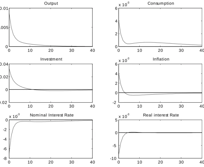
100

basis point decrease in the annualized nominal interest rate. The rate of in‡ation as well as the real interest rate are also annualized. All other variables are measured as the respective log deviation of the original variable from its steady state value. Fig.

2

illustrates the outcome under the baseline calibration. Monetary policy shocks are shown to lead to strong and persis- tent dynamic responses of the variables under consideration. How do they compare to those estimated using structural vector autoregressive (SVAR) methods?

⁹

The estimates reported by Christiano et al. (2005) indicate that the maximum output response to an identi…ed monetary policy shock is about

0:5

percent (with

95

per- cent con…dence interval around this point estimate of about

0:2). After that,

output is estimated to take about one and a half years to revert to its original level.

Christiano et al. (2005) also estimate a maximum investment response of about one percent (with

95

percent con…dence interval around this point estimate of about

0:5). The estimated maximum consumption response is roughly0:2

percent (with

95

percent con…dence interval around this point estimate of about

0:1) while the

estimated maximum in‡ation response of roughly

0:2

percent (with

95

percent con-

…dence interval around this point estimate of about

0:15). Finally, the nominal

interest rate takes about two quarters to return half-way to its preshock level.

[Figure

2

about here]

By and large, the theoretical impulse responses shown in Fig.

2

are similar to the empirical evidence on the dynamic consequences of monetary policy shocks. An exception is investment. In fact, the (about) three percent impact response to the shock is out of line with the point estimate of one percent for the maximum response of that variable. In a way that is consistent with the large size of the investment response, the impact responses of the remaining real quantities also turn out to be somewhat to the high part of the empirically plausible range. On the positive side we can notice, however, that the impact responses of the nominal variables are better in line with corresponding point estimates of the maximum responses. We also …nd that the dynamic consequences of the shock are reasonably persistent. What is the relevance of this result, and what is the economic mechanism at work? Woodford

9It is precisely that comparision which is routinely used by proponents of NK theory to justify the quantitative relevance of this framework. See, e.g., the discussion in Galí (2015), p.68 in the context of a model featuring a constant capital stock at the …rm level.

(2005) shows that a NK model featuring a convex capital adjustment cost at the

…rm level gives rise to a quantitatively relevant monetary transmission mechanism.

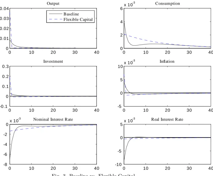
On the other hand, Carlstrom and Fuerst (1997) show that for a constant level of net worth the agency-cost model implies a smoothing mechanism that is analogous to the one implied by a convex capital adjustment cost. As it turns out, in the context of our model, that smoothing mechanism is remarkably strong. In order to substantiate the latter statement, we shut down the …nancial friction by setting the bankruptcy cost, , to a very small value. Investment is therefore fully ‡exible in this case and the implied dynamic responses of the variables under consideration to the monetary policy chock are illustrated in Fig.

3. Let us also notice that

parameters ,

c_e

and are adjusted in such a way that the same objects as in our baseline calibration are still targeted.

[Figure

3

about here]

The results shown in Fig.

3

help explain the relevance of our baseline results. In fact, the impulse responses document the well known problem that ‡exible invest- ment gives rise to counterfactual impulse responses to monetary policy shocks. This is exactly the reason why Christiano et al. (2005) and Woodford (2005) had intro- duced adjustment costs into the investment block of the NK framework. In their work there is, however, no empirical discipline imposed on the size of the adjustment cost, apart from a desire to parametrize the postulated cost in a way that gives rise to a realistic monetary transmission mechanism. This is true for both the invest- ment adjustment cost in Christiano et al. (2005), as well as for the convex capital adjustment cost in Woodford (2005). On the contrary, the size of the …nancial fric- tion in our model is disciplined by data on interest rate spreads, bankruptcy rates and bankruptcy costs, as explained in section

3:1. It is therefore remarkable that

a …nancial friction of a plausible size implies a strong smoothing mechanism that makes our baseline results go a long way towards a realistic monetary transmission mechanism. Let us also inspect some quantitative aspects of Fig.

3. The impact

investment response to the monetary policy shock turns out to be almost twenty percent, i.e., twenty times larger than the corresponding maximum point estimate reported by Christiano et al. (2005). In the NK lumpy investment model proposed in Reiter (2013) we found a counterfactual monetary transmission mechanism with an impact investment response of about eight percent.

¹⁰

Compared with the twenty percent impact response implied by the ‡exible capital model we …nd that a standard (S,s) modelling of lumpy investment does imply a (modest) smoothing mechanism.

¹¹

10This is for the case of Calvo pricing combined with (S,s) investment.

11Strictly speaking, the irrelevance result in Thomas (2002) and Kahn and Thomas (2008) does

This points to the possibility that a standard modelling of lumpy investment could overcome the remaining problem with a somewhat too ‡exible investment under our baseline calibration. Below we inspect the robustness of our results by varying the form of the …nancial friction in various ways. Discussing the di¤erences with respect to our baseline allows us to further inspect the economic mechanisms at work.

3.3 Robustness Analysis

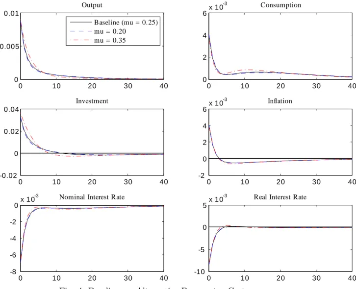
The …rst robustness analysis regards the size of the …nancial friction.

¹²

More con- cretely, we now consider values for the bankruptcy cost, , that are to the high and to the low part of the empirically relevant range. This is illustrated in Fig.

4.

Each line in the …gure is associated with one value of

2 f0:2, 0:25, 0:36g

, and parameters ,

c_e

and are adjusted in such a way that the same objects as in our baseline calibration are still targeted.

[Figure

4

about here]

Fig.

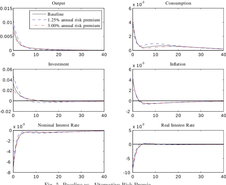
4

brings out a clear message. Our baseline results are robust with respect to reasonable variations in the size of the …nancial friction. A related question regards the quantitative importance of our baseline choice for the annual risk premium in the steady state. This is addressed in Fig.

5.

[Figure

5

about here]

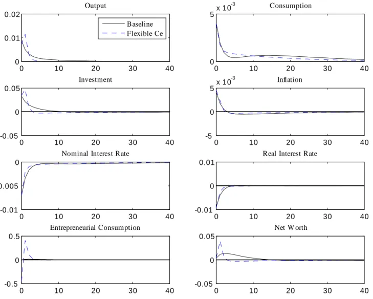
The investment response to the shock becomes smaller if the size of the …nancial friction, as measured by the risk premium, is increased. However, even in the case of a three percent annual risk premium the associated impact responses to the mone- tary policy shock remain somewhat counterfactual. The main problem is once again seen to be the large ‡exibility in investment. Finally, we examine the original mod- elling of the …nancial friction in Carlstrom and Fuerst (1997). In order to guarantee that the above mentioned contracting problem between entrepreneurs and the CMF is well-de…ned at each point in time, one has to make sure that entrepreneurs do not accumulate net worth to the point that this problem simply disappears. Carlstrom and Fuerst (1997) achieve this by assuming that entrepreneurs discount the future

therefore not go through in the context of a NK model. In fact, those authors had established an equivalence in the equilibrium determination of aggregate quantities between a (S,s) modelling of lumpy investment and a frictionless RBC model.

12A robustness analysis with respect to the monetary policy parameters just plays out in ways that are similar to the corresponding outcomes in standard NK models. The same is true for variations of the price stickiness parameter. Let us also notice that the baseline results turn out to be robust with respect to our choice of steady state in‡ation. Needless to say, those results are available upon request.

more heavily than do households. The entrepreneur’s Euler equation is therefore of the form

qt = Etf[qt+1(1 ) +rt+1]roit+1g;

(20) where parameter re‡ects the assumption that entrepreneurs discount the future more heavily than households. We set this parameter to

0:947. Otherwise, all para-

meters and steady state values are the same as in our baseline. The last equation also re‡ects that entrepreneurs are assumed to be risk-neutral. The associated monetary transmission mechanism is illustrated in Fig.

6.

[Figure

6

about here]

Compared with the baseline, the theoretical impulse responses, as implied by the Carlstrom and Fuerst (1997) assumption on entrepreneurial consumption, are further away from their empirical counterpart. In fact, the maximum investment response to the shock is now more than four percent, compared with about three percent in the baseline, and the one percent maximum response in the data. The economic reason is the large extent to which risk-neutral entrepreneurs engage in intertemporal consumption substitution implying highly volatile equilibrium invest- ment dynamics. This is seen in Fig.

6. An expansionary monetary policy shock

gives rise to an increase in aggregate demand in the economy. Firms are therefore incentivized to produce more and consequently increase their demand for capital and labor. The persistent increase in the demand for capital leads to an increase in its price. The latter results in an increased return on investment which gives entrepreneurs the incentive to reduce their consumption. Starting one period after the monetary policy shock entrepreneurs increase their consumption again. The reason is that they can enjoy an increased net worth by that time, and the relative attractiveness of investing (as opposed to consuming) declines, as the dynamic con- sequences of the monetary policy shock start fading out. Overall, Fig.

6

conveys a clear message. The assumed form of the …nancial friction matters for the implied monetary transmission mechanism, and this in itself makes it highly desirable to further improve the micro-foundations of quantitative macroeconomic models along that dimension.

4 Conclusion

Once New Keynesian (NK) theory (see, e.g., Woodford 2003) is combined with

a standard model of investment (see, e.g., Thomas 2002), the resulting framework

loses its ability to generate a realistic monetary transmission mechanism. This is the

puzzle uncovered in Reiter et al. (2013). The simple economic reason behind it is the high degree of ‡exibility in capital accumulation, as implied by standard investment theory. We therefore ask how to reconcile ‡exibility in capital accumulation with a quantitatively relevant monetary transmission mechanism. In order to address this question, we develop a NK model featuring fully ‡exible investment combined with a …nancial friction in the spirit of Carlstrom and Fuerst (1997). This simple model is shown to go a long way towards a realistic monetary transmission mechanism.

It can therefore be expected that in the presence of an empirically plausible

…nancial friction of the type considered in this paper, standard investment theory can be integrated into an empirically relevant NK model of the monetary transmission mechanism. This is the next natural step in this agenda. The interest is twofold.

First, it is an open question whether standard normative lessons from NK theory

hold up in the presence of lumpy investment. The reason is that lumpy investment is

a potential source of signi…cant heterogeneity across …rms. Hence, it might play an

important role in shaping the optimal monetary policy response to shocks, the same

way staggered prices generate ine¢ cient price dispersion and thus provide a motive

for in‡ation stabilization. Sveen and Weinke (2016) make some progress on that

front, however in the context of a simple Calvo (1983) style model of investment à la

Sveen and Weinke (2007). Second, in order to increase the empirical relevance of the

monetary transmission mechanism with respect to standard textbook treatments a

rich set of additional features has been proposed. Prominent among them is an

investment adjustment cost à la Christiano et al. (2005). But the existence of this

adjustment cost makes NK models inconsistent with the observed lumpiness in plant-

level investment. It is therefore an open question how to match the quantitative

features of estimated impulse responses to a monetary policy shock without relying

on assumptions that eliminate micro-level lumpiness in investment.

References

Bernanke, B., Gertler, M., Gilchrist, S., 1999. The Financial Accelerator in a Quan- titative Business Cycle Framework. In: Taylor, J., Woodford, M. (Eds.), Handbook of Macroeconomics. Vol. 1. Elsevier, Amsterdam, Netherlands, pp. 1341-1393.

Caballero, R.J., Engel, E.R.M.A., 2007. Price Stickiness in Ss Models: New Inter- pretations of Old Results. Journal of Monetary Economics 54S, 100–121.

Calvo, G., 1983. Staggered Prices in a Utility Maximizing Framework. Journal of Monetary Economics 12, 383-398.

Carlstrom, C.T., Fuerst, T.S., 1997. Agency Costs, Net Worth, and Business Fluc- tuations: A Computable General Equilibrium Analysis. American Economic Review 87, 893-910.

Carlstrom, C.T., Fuerst, T.S., 2001. Monetary Shocks, Agency Costs, and Business Cycles. Carnegie-Rochester Conference Series on Public Policy 54, 1-27.

Christiano, L.J., Eichenbaum, M., Evans, C.L., 2005. Nominal Rigidities and the Dynamic E¤ects of a Shock to Monetary Policy. Journal of Political Economy 113, 1-45.

Doms, M., Dunne, T., 1998. Capital Adjustment Patterns in Manufacturing Plants.

Review of Economic Dynamics 1, 409–429.

Galí, J., 2015. Monetary Policy, In‡ation, and the Business Cycle: An Introduction to the New Keynesian Framework. 2nd Edition. Princeton University Press.

Khan, A., Thomas, J.K., 2008. Idiosyncratic Shocks and the Role of Nonconvexities in Plant and Aggregate Investment Dynamics. Econometrica 76, 395-436.

Reiter, M., 2009. Solving Heterogeneous-Agent Models by Projection and Pertur- bation. Journal of Economic Dynamics and Control 33, 649-665.

Reiter, M., 2010. Approximate Aggregation in Heterogeneous-Agent Models. IAS Economics Working Paper 258.

Reiter, M., Sveen, T., Weinke, L., 2013. Lumpy Investment and the Monetary Transmission Mechanism. Journal of Monetary Economics, 60, 821–834.

Sveen, T., Weinke, L., 2007. Lumpy Investment, Sticky Prices, and the Monetary Transmission Mechanism. Journal of Monetary Economics 54S, 23-36.

Sveen, T., Weinke, L., 2016. Optimal Monetary Policy with Nominal Rigidities and

Lumpy Investment. Forthcoming International Journal of Central Banking.

Thomas, J.K., 2002. Is Lumpy Investment Relevant for the Business Cycle? Journal of Political Economy 110, 508-534.

Woodford, M., 2003. Interest and Prices: Foundations of a Theory of Monetary Policy. Princeton University Press.

Woodford, M., 2005. Firm-Speci…c Capital and the New-Keynesian Phillips Curve.

International Journal of Central Banking 1, 1-46.

Fig. 1. A Bird’s View on the Model.

0 10 20 30 40 0

0.005 0.01

Output

0 10 20 30 40

0 2 4

6x 10^-3 Consum pti on

0 10 20 30 40

-0.02 0 0.02 0.04

Investm ent

0 10 20 30 40

-2 0 2 4

6x 10^-3 Inflation

0 10 20 30 40

-8 -6 -4 -2

0x 10^-3 Nom i nal Interest Rate

0 10 20 30 40

-10 -5 0

5x 10^-3 Real interest Rate

Fig. 2. Dynamic Responses to a Monetary Policy Shock: Baseline.

0 10 20 30 40 0

0.01 0.02 0.03 0.04

Output

Baseline Flexible Capital

0 10 20 30 40

0 2 4

6x 10^-3 Consumption

0 10 20 30 40

-0.1 0 0.1 0.2 0.3

Investment

0 10 20 30 40

-5 0 5

10x 10^-3 Inflation

0 10 20 30 40

-8 -6 -4 -2

0x 10^-3 Nominal Interest Rate

0 10 20 30 40

-10 -5 0

5x 10^-3 Real Interest Rate

Fig. 3. Baseline vs. Flexible Capital.

0 10 20 30 40 0

0.005 0.01

Output

Baseline (mu = 0.25) mu = 0.20

mu = 0.35

0 10 20 30 40

0 2 4

6x 10^-3 Consumption

0 10 20 30 40

-0.02 0 0.02 0.04

Investment

0 10 20 30 40

-2 0 2 4

6x 10^-3 Inflation

0 10 20 30 40

-8 -6 -4 -2

0x 10^-3 Nominal Interest Rate

0 10 20 30 40

-10 -5 0

5x 10^-3 Real Interest Rate

Fig. 4. Baseline vs. Alternative Bancruptcy Costs.

0 10 20 30 40 0

0.005 0.01 0.015

Output Baseline

1.25% annual risk premium 3.00% annual risk premium

0 10 20 30 40

0 2 4

6x 10^-3 Consumption

0 10 20 30 40

-0.02 0 0.02 0.04 0.06

Investment

0 10 20 30 40

-2 0 2 4

6x 10^-3 Inflation

0 10 20 30 40

-8 -6 -4 -2

0x 10^-3 Nominal Interest Rate

0 10 20 30 40

-10 -5 0

5x 10^-3 Real Interest Rate

Fig. 5. Baseline vs. Alternative Risk Premia.

0 10 20 30 40 0

0.01 0.02

Output

Baseline Flexible Ce

0 10 20 30 40

0

5x 10^-3 Consumption

0 10 20 30 40

-0.05 0 0.05

Investment

0 10 20 30 40

-5 0

5x 10^-3 Inflation

0 10 20 30 40

-0.01 -0.005 0

Nominal Interest Rate

0 10 20 30 40

-0.01 0 0.01

Real Interest Rate

0 10 20 30 40

-0.5 0 0.5

Entrepreneurial Consumption

0 10 20 30 40

-0.05 0 0.05

Net W orth

Fig. 6. Baseline vs. Carlstrom Fuerst Ass. on Entrepreneurial Consumption.