19 Eastern European Business and Economics Journal Vol.1, No. 3, (2015): 19-47
Jenny Koerner University of Regensburg
Universitätsstr. 31, 93053 Regensburg, Germany Tel.: +49 941 943 2708
Jenny.Koerner@ur.de
Reviewers:
Mohamed Ben MIMOUN, Umm Al-Qura University, Saudi Arabia;
Kevin SALYER, University of California, Davis USA;
Sebastian UTZ, University of Regensburg, Germany.
Abstract
This paper analyzes the transmission mechanisms of a contractionary monetary policy shock on the real economy. The sufficiently long regime uniform time period since the political transformation in the Czech Republic provides evidence for effective inflation targeting by the Czech National Bank. I apply a recursive vector autoregression (VAR), a structural VAR, and structural vector error correction model (SVECM). In the SVAR the restrictions imply a lagged effect of the monetary policy shock on output and prices in the short run, and money neutrality in the long-run. In the SVECM a money demand and an interest rate relationship identify the cointegrating vectors. The impulse responses of all models state a reduction of output and consumer prices after monetary tightening. The exchange rate overshoots its steady state level in the VAR and SVECM models, indicating a large degree of exchange rate volatility after the shock. The results reveal an interest pass-through from Czech monetary policy to inflation.
Keywords: monetary transmission, Czech Republic, Structural VAR, Structural VECM, Cointegration, price puzzle
Introduction
After the transition to a free market system in the post-communist Czech Republic, the Czech National Bank adopted a monetary policy that targets an explicit inflation rate. A change in the policy interest rate modifies inflation and real variables through various channels. Vector autoregression (VAR) models are used to analyze the speed and the degree of the transmission. The development of the financial and banking systems has altered the monetary transmission mechanisms in the Czech Republic. The empirical analysis ranging over sufficiently long data set that is uniform across regimes provides insights into the changed transmission mechanisms. The results reveal a more symmetric
transmission mechanism to countries of the Eurozone than earlier studies.
In comparison with other Central and Eastern European countries, the Czech financial market advanced quickly after the transition. The two- stage banking system with commercial banks and an independent central bank replaced the communist structures and the liberalisation of the capital market in a matter of course. The Czech Republic pursues inflation targeting and has followed a flexible exchange rate system since 1997. The fast progress of the monetary and financial system in the Czech Republic accompanies the evolution of the monetary transmission mechanism.
Egert and MacDonald (2009) comprehensively summarize the main empirical studies to transmission channels in Eastern Europe. The analysis of Ganev et al. (2002) is among the first comprehensive studies of East Europe, including the Czech Republic, after the transformation.
They state that the pass-through of monetary policy to the real economy is rather imperfect. The underdeveloped institutions in this early phase of the transformation might justify this finding. Several authors found evidence for a price puzzle in the post-communist countries (Arnostova and Hurnik, 2005; Creel and Levasseur, 2005). A price puzzle refers to the positive reaction of the price level after a monetary policy shock that is not in line with macroeconomic theory. My study is similar to Borys et al. (2009), who estimate a VAR, structural VAR (SVAR), a factor- augmented VAR, and a Bayesian VAR. They document a well- functioning transmission mechanism symmetric to countries of the European monetary union (EMU). They find no price puzzle. They conclude that data from a single monetary policy regime eliminated the paradoxical result. I will confirm this finding with my results.
Additionally, my analysis covers a decent long time period, allowing to conduct a SVAR with long run restrictions and to account for cointegration relations within the Czech data set. To best of my knowledge, this is a gap in literature until now.
In this paper, the five-dimensional monthly data set ranges from the beginning of 1999 to September 2011 and comprises output, inflation, money supply, and the key interest rate, as well as the nominal exchange rate between the Koruna and the Euro. Since the Czech Republic is a small open economy, the relationships used for the identification of the models are based on the basic economic relationships of the Mundell- Fleming-Dornbusch model (Dornbusch, 1976). The focus of the analysis
is to evaluate the effect of a contractionary monetary policy shock on real variables and inflation. Monetary policy shocks refer to the unsystematic part of a change in the monetary policy instrument. I check the variables’
effects for symmetry with the reactions predicted by the Mundell- Fleming-Dornbusch model after monetary tightening. The results are of particular interest, since the countries of Eastern European enlargement have no opting-out clause from the EMU (there has been considerable opposition by the Czechs against the adoption of the Euro at the moment.). The countries are obliged to adopt the Euro eventually by the terms of their accession treaties. Since membership in the Exchange Rate Mechanism (ERM) is a prerequisite for the Euro adoption, and joining ERM is voluntary, the Czech Republic can ultimately control the timing of their adoption of the Euro by deliberately not satisfying the ERM requirement. Symmetric monetary transmission mechanisms with the Eurozone countries would be an important factor to ensure an effective monetary policy by the European Central Bank.
In VAR models, restrictions are necessary to identify a monetary policy shock and to allow an economic interpretation. Since exogenous imposed restrictions depict the structure of the underlying economic relationships, I use three different model types to analyse monetary transmission in the Czech Republic and to ensure robust results. A recursive, semistructural VAR is based on a Cholesky decomposition. In a SVAR with long and short-run restrictions, the monetary policy affects output and prices with a time lag, and the long-run restrictions define monetary neutrality. These assumptions are in compliance with economic theory. Similarly, the restrictions in the structural vector error correction model (SVECM) are set to regard an interest rate and money demand relationship as long-run relations within the data set.
The results of this study reveal an effective pass-through of Czech monetary policy actions to the price level without signs of a price puzzle.
In all models output and prices decrease after monetary tightening in line with the interrelations in the Mundell-Fleming-Dornbusch model. The effects of output are, however, associated with great uncertainty. The monetary policy transmission in the Czech economy shows symmetry to the transmission in EMU countries. Earlier studies could not confirm this finding. This result supports a Czech accession to the EMU which is however unlikely at the moment. Two of three models document a delayed overshooting of the exchange rate indicating high nominal exchange rate volatility. The gradual appreciation of the nominal
exchange rate since 1999 might have caused this result. The similar sign effects in the VAR, SVAR and SVECM model back the robustness of my results. The SVECM generates more persistent reactions than the models based on a VAR estimation.
In the next section I will introduce the method of VAR and vector autoregression models (VECM). The empirical analysis follows with the description of the data set and the estimation of the models including the identification of the SVECM. Subsequently, the model results are presented and interpreted. In the conclusion the main insights are summarized.
Method
VAR models are tools commonly applied to analyze the effects of monetary policy shocks. Vector autoregression models characterize merely endogenous variables and stationary time series. On the contrary, VECM models are based on integrated variables. I apply the different model specifications to formally verify the theory of the Mundell- Fleming Dornbusch model on the basis of empirical data from the Czech Republic and to learn from the past dynamic of economic variables (Lütkepohl, 2005).
Structural Vector Autoregression
A VAR (p) is a multivariate simultaneous equation model with p lagged values of the variables under consideration. The structural form is:
ܣݔ௧ = ܥଵݔ௧ିଵ+ ܥଶݔ௧ିଶ+ … + ܥݔ௧ି+ ܤߝ௧
The ሺ݇ × 1ሻ vector ݔ௧ contains the endogenous variablesand their lagged values ݔ௧ି. ߝ௧ is the ሺ݇ × 1ሻ vector of shocks. The ሺ݇ × ݇ሻ matrices ܣ, ܥ and ܤ express the contemporary relationships between the variables, the coefficient matrix for the corresponding lags (݈ = 1, … ሻ, and respectively the linear relationship between the vector of shocks ߝ௧. The single shock ߝ௧ characterizes orthogonality to each other and unit variance:
ܸܽݎሺߝ௧ሻ = Ωఌ = 1 … 0
⋮ ⋱ ⋮ 0 … 1൩
However, only the reduced VAR representation can be estimated:
ݔ௧ = Ψଵx୲ିଵ+ Ψଶx୲ିଶ+ ⋯ +Ψ୮x୲ି୮ + u୲
with the matrix Ψ = ܣିଵܥ and the residual vector ݑ௧ = ܣିଵܤߝ௧. The identification problem arises because the residuals are a linear transformation of the white noise vector ߝ௧. The residuals ݑ௧ for the k variables are correlated within the system. Since macroeconomic variables are likely to be correlated with each other, the residuals of the variables’ equations are also correlated:
ܸܽݎሺݑ௧ሻ = Ω௨ = ߪଵଶ … ߪ
⋮ ⋱ ⋮
ߪ … ߪଶ
Additional restrictions are needed to identify the shocks from the residuals. To solve the identification problem, I set A as an identity matrix and set ሺିଵሻ
ଶ restrictions in B. The restrictions affect the contemporary relationship between the shocks and the corresponding variables. In the recursive VAR the B matrix is lower triangular (Sims, 1980). In the SVAR, I set short and long-run restrictions. The restrictions in B, for example ܾ = 0 prevents that shock k affects variable j within the same period. Restrictions in the impact matrix influence the long-run evolution of shocks.
If the VAR(p) model is stationary, there exists a Moving-Average (MA) representation according to Wold’s theorem (Lütkepohl and Krätzig, 2004). The dependence of the variables in ݔ௧ from the orthogonal shocks facilitated the interpretation, because the residuals do not occur in isolation.
The impulse responsesillustrate the dynamic of a shock through the system (Lütkepohl and Krätzig, 2004). Summarizing Φ୧ = Ψܣିଵܤ for all i=1,2,3..., I can derive the impact multipliers Φthat allow long-run restrictions.
ݔ௧= Φߝ௧ି
ஶ
ୀ
The parameter Φሺሻ describes the reaction of variable j on a one standard deviation change of the k’s shock that occurred i periods ago. The uncorrelated shocks are isolated through the relationship ݑ௧= ܣିଵܤߝ௧ (Lütkepohl, 2005). The variance-covariance matrix of the residuals can be represented with the matrix B and Ωக, Ω௨ = ܤΩகܤᇱ.
Applying the Cholesky decomposition the factorization of the residual covariance matrix results in a product of lower triangular
matrices. Substituting Ωఌ by ܫ and normalizing the diagonal elements of B, so that ܤିଵΩ௨ ܤᇱିଵᇱ= ܫthe triangular structure is evident. Thus, the relationship between the variables depends on their ordering, creating a causal chain system.
In the SVAR, the short-run restrictions are set in the B matrix in a non-recursive way in line with economic theory. The long-run restriction in Φ are subject to a particular structural decomposition (Blanchard and Quah, 1989). The rationale behind the restrictions in the SVAR is introduced in the section on the identification.
Structural Vector Error Correction Model
Most macroeconomic variables exhibit a stochastic trend. A VECM incorporates the cointegrating relationship between the variables and regards it as a single long-run relationship. Assuming only variables integrated of order one I(1), the reduced form representation of a VECM(p) is given by
Δݔ௧ = Πݔ௧ିଵ+ ΓଵΔx୲ିଵ+ … + Γ୮ିଵΔx୲ି୮ାଵ+ u୲
while p is the number of lags included. Δݔ௧ contains the stationary first differences of the variables, Πݔ௧ିଵ includes the cointegrating relationships and is also stationary. Γ୧ for ݅ = 1, … , − 1 encompasses the short-run coefficients. The residuals u୲ are in general correlated with each other.
Π itself is of reduced rank. The decomposition in Π = αβᇱ yields two matrices, ߙ and ߚ ,with full rank. The cointegratng relationship is encompassed in ߚᇱݔ௧ିଵ. ߙ is the loading matrix representing the weights of each cointegration relation (Neusser, 2009). The matrices ߙ and ߚ are not unique. The cointegrating vectors are however identifiable with ݎሺݎ − 1ሻ restrictions based on economic theory in ߚ.
The MA-representation of a reduced form VECM subject to the shocks is:
ݔ௧= ΞAିଵB ߝ + Ξ∗ܮ
ஶ
ୀ
௧
ୀଵ
ܣିଵܤߝ௧+ ݕ∗
The first part including the cointegration relation does not converge to zero with ݅ → ∞. The part depicts the permanent effect of a shock. The infinite order polynomial with the Lag operator illustrates the transitory effects, since it converges to zero with j→ ∞. The term ݕ∗ includes the
initial values. As it has been the case in the VAR, the shocks have to be identified with ݑ௧= ܣିଵܤߝ௧ for a meaningful impulse response analysis.
The identification of the system is twofold. The determination of the cointegration rank r of Ξ provides the information about the ሺ݇ − ݎሻ permanent ߝand the r transitory shocks ߝ் (Brüggemann, 2003).
For the VECM, I assume that B is a unitary matrix. First, the short- run restrictions Ξ∗~ = Ξ∗ܮܣିଵܤߝ௧are declared as in the stationary VAR case with ሺିଵሻ
ଶ restrictions in A. Second, I summarize Ξ~ = ΞAିଵB. I reorder Ξ~, so that the transitory shocks are clustered with the zero vectors in the first columns ሺ݇ × ݎሻ. In the (݇ × ሺ݇ − ݎሻ) remaining columns of Ξ~ the permanent shocks have to be identified by
ሺ×ሻሺିିଵሻ
ଶ additional zero-restrictions.
In the (S)VAR and the SVECM the focus is the orthogonalisation of residuals by identifying restrictions.
Identification
The restrictions in a VAR, SVAR, and SVECM underlie the appraisal of the researcher unless there is some justification from subject matter theory (Lütkepohl and Krätzig, 2004). The relations in the Mundell- Fleming-Dornbusch Model build the foundation of the restrictions used here (Dornbusch, 1976). The variable set ݔ௧ = ሾܻ௧, ߨ௧, ܯ௧, ݅௧, ܧ௧ሿ comprises of output, a price variable, the real money supply, the nominal interest rate, and the exchange rate. The well-known steady-state conditions corresponding to the variables are the Phillips curve, an aggregated demand equation, a money demand and supply equation, as well as the uncovered interest parity condition. to determine the exchange rate. The restrictions enable to interpret the non-systematic part of a key interest change – the monetary policy shock. I use different model identification schemes to prevent that the results exhibit a modelling bias.
Recursive VAR identification
In the recursive VAR, the ordering of the five variables is crucial. The induced causal chain leans against Peersman and Smets (2001) and Bjornland (2008). The ordering ݔ௧ = ሾܻ௧, ߨ௧, ܯ௧, ݅௧, ܧ௧ሿ′ implies that domestic variables such as output, prices and the real money supply react
to a monetary policy shock with a time lag. But shocks of macroeconomic variables affect policy variables and the exchange rate instantaneously. Thus, the monetary policy shock ߝெ has only an instantaneous effect on the interest rate itself and on the exchange rate.
With this structure, the shock to output depicts an aggregate supply shock ߝௌand affects all variables contemporaneously. The shock to prices ߝூௌ
is assumed to be an aggregate demand shock which affects all variables besides output. A change in the money demand ߝெ influences the real money supply as well as the policy variable and the exchange rate. Since the exchange rate is weakly exogenous due to possible foreign influence, I place the nominal exchange rate last. ߝா௫ affects all variables with a lag. This procedure is in line with Bernanke and Mihov (1998) and Bjornland (2008).
ۏێ ێێ ۍݑݑగ
ݑெ ݑூ ݑாےۑۑۑې
= ۏێ ێێ
ێۍܾ,ௌ 0 0 0 0
ܾగ,ௌ ܾగ,ூௌ 0 0 0
ܾெ,ௌ ܾெ,ூௌ ܾெ,ெ 0 0
ܾூ,ௌ ܾூ,ூௌ ܾூ,ெ ܾூ,ெ 0
ܾா,ௌ ܾா,ூௌ ܾா,ெ ܾா,ெ ܾா,ா௫ےۑۑۑۑې ۏێ ێێ ۍߝௌ
ߝூௌ
ߝெ
ߝெ
ߝா௫ےۑۑۑې SVAR with long and short-run restrictions
The identification in a SVAR with long and short-run restrictions allows a more sophisticated identification of the shocks (Gali, 1992).
The long-run restrictions are set in the Φௌோ of the model. A main insight of macroeconomics is money neutrality, i.e. an increase in the money supply has no long-run effect on real variables, but generates inflation (Lastrapes, 1998). A monetary policy shock changes money supply. Therefore I assume the monetary policy shock does not have an effect on the real money aggregate and output in the long run, codified by zeros in Φௌோ. With this assumption, the nominal interest rate is inversely related to the money aggregate M2. M2, however, includes more monetary components beyond monetary reserves that are controllable by the monetary policy authority. The effect of a money demand shock involves a change in the money supply. The money neutrality assumption eliminates real consequences of a money demand shock in the long run (King and Watson, 1997). In line with Blanchard and Quah (1989) the aggregate demand shock has only a transitory effect on real output. Thus the assumptions Φ,ூௌ = Φ,ெ = Φ,ெ =
Φெ,ெ= 0 rely on a long-run vertical Phillips curve. Just aggregate supply and aggregate demand shocks change output permanently.
ۏێ ێێ ۍݑݑగ
ݑெ ݑூ ݑாےۑۑۑې
= ۏێ ێێ
ێۍܾ,ௌ ܾ,ூௌ 0 0 0
ܾగ,ௌ ܾగ,ூௌ 0 0 0
ܾெ,ௌ ܾெ,ூௌ ܾெ,ெ ܾெ,ெ ܾெ,ா௫
ܾூ,ௌ ܾூ,ூௌ ܾூ,ெ ܾூ,ெ ܾூ,ா௫
ܾா,ௌ ܾா,ூௌ ܾா,ெ ܾா,ெ ܾா,ா௫ےۑۑۑۑې ۏێ ێێ ۍߝௌ
ߝூௌ
ߝெ
ߝெ
ߝா௫ےۑۑۑې
Φௌோ = ۏێ ێێ
ێۍϕ,ௌ 0 0 0 ߶,ா௫
߶గ,ௌ ߶గ,ூௌ ߶గ,ெ ߶గ,ெ ߶గ,ா௫
߶ெ,ௌ ߶ெ,ூௌ ߶ெ,ெ 0 ߶ெ,ா௫
߶ூ,ௌ ߶ூ,ூௌ ߶ூ,ெ ߶ூ,ெ ߶ூ,ா௫
߶ா,ௌ ߶ா,ூௌ ߶ா,ெ ߶ா,ெ ߶ா,ா௫ےۑۑۑۑې
Further, six restrictions prevent contemporaneous reactions in the system, set in the B-matrix. Again, price rigidity is assumed by not allowing nominal shocks to affect real variables and inflation contemporaneously. Nominal shocks comprise the monetary demand and supply shock and the exchange rate shocks. The observable correlation of the monetary policy rate and the nominal money supply shows that a change of the monetary policy instrument influences the real money supply in the short run. The policy interest rate reacts to all shocks including the exchange rate implied by the fourth line. The monetary policy should not per se react to sudden changes of the exchange rate, but a limited reaction on exchange rate fluctuations is justifiable (Arnostova and Hurnik, 2005). In the Czech Republic, as a small open economy, shocks to the exchange rate modify the nominal money supply. In reverse, a shock to the money supply or the policy rate affects the nominal exchange rate. All shocks differ with this identification and are consistent with the general argumentation of macroeconomic theory.
In the next section, the impulse response analysis will expose whether a contractionary monetary policy shock also generates reactions that are comparable to the theory implications of the Mundell-Fleming- Dornbusch model.
The empirical analysis
The choice to analyse the Czech Republic has a couple of reasons. The Czech National Bank, independently from fiscal policy, pursues with its
objective on price stability a credible monetary policy according to the World Bank report (Mitra et al., 2010). Since the 2000s the Czech Republic marked nominal interest rates below the interest rate of the Euro area. Despite the exchange rate appreciation with the productivity growth, loans in local currency were thus more attractive than loans in foreign currency. During the catch-up process in the Czech Republic, no high inflation rate was observable that the Samuelson effect would imply and characterized neighbour countries. There are also no signs that the high fraction of foreign commercial banks impedes the monetary transmission. The Czech National Bank advocates not to manipulate the exchange rate in favour for the distinct Czech export sector (over 70 % of GDP) (Mitra et al., 2010). Thus, the economy is stable enough to adjust to shocks from abroad. The study of Coricelli et al. (2006) documents that the exchange rate pass-through is the lowest in the Czech Republic of the Central and Eastern European countries. The shock- absorbing effect of the exchange rate between the Czech koruna and the Euro and the positive institutional framework suggest that the monetary transmission mechanisms are consistent with economic theory in the Czech Republic.
Data
The minimal variable choice dictates the typical time series to analyze the monetary transmission mechanism. The monthly data set ranges from January 1999 to September 2011. In the end of 1998 the Czech National Bank switched to inflation targeting. Since 1997 the country has pursued a flexible exchange rate regime. The year 1998 was characterized by a banking crisis. That is why I choose January of 1999 as the starting date for the examination, which is uniform across regimes.
Table 7 provides the information about the data sources and possible corrections. The economic activity Y represents the seasonal adjusted real gross domestic product, RGDP. I use the interpolation method of Chow Lin, so that the average of the monthly interpolated date matches the quarterly observation.
The monthly total consumer price index, CPI, is used for the calculation of the price growth rate ߨ. The consumer price index includes the prices of imported goods contrary to the GDP deflator. The non- adjusted nominal money supply M2 is deflated by the CPI to serve as the real money supply, RM2.Including the real instead of the nominal money supply excludes the money supply as an instrument of the central bank
and ensures the separation between a money supply and a money demand shock.
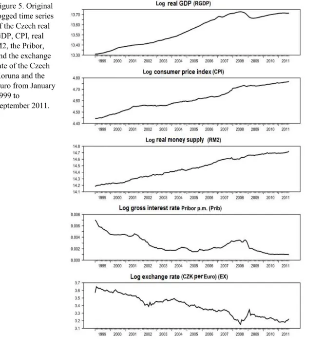
The Prague interbank offered rate (Pribor, or Prib) is used as the monetary policy rate. The 2-weeks repo rate is the official monetary instrument, but it is not continuously adjusted; this, Iuse the Pribor. The correlation between the Pribor and the 2-week repo rate is 0.98940. The exchange rate is the rate of exchange between the Czech Koruna and the Euro in direct quotation, Ex. Seasonally unadjusted time series are adjusted by X11 procedure. The Figure 5 shows the original log of all variables.
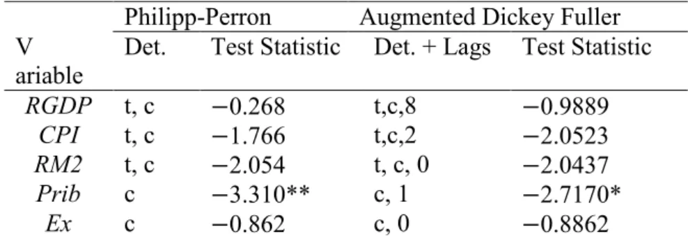
I apply the Phillips-Perron and Augmented Dickey Fuller unit root tests to all variables, including a constant. The results are summarized in Table 1. A unit root in the time series of the Prib can be rejected with both tests. All other variables are subject to a unit root. Stationary variables are necessary for a consistent VAR estimation. Therefore, I transform the remaining variables. The per month inflation rate is a stationary representation of the CPI. For consistency, all rates base on a month. I apply the Demean-Remean method on the variables RGDP, M2 and Ex to obtain stationary variables while keeping some level information. For this approach, I apply the Hodrick Prescott filter and add the arithmetic mean to the de-trended time series. The proportionality between the RGDP and M2 is retained in line with the quantity equation. The transformed data are denoted with an additional C.
Philipp-Perron Augmented Dickey Fuller V
ariable
Det. Test Statistic Det. + Lags Test Statistic RGDP t, c −0.268 t,c,8 −0.9889
CPI t, c −1.766 t,c,2 −2.0523
RM2 t, c −2.054 t, c, 0 −2.0437
Prib c −3.310** c, 1 −2.7170*
Ex c −0.862 c, 0 −0.8862
Note: Det.: deterministic component; t = trend; c = constant; asterisks (*) denote, that the zero hypothesis is rejected on a 10 % (*), on a 5 % (**) or a 1 % (***) significance level. The lag length in the Augmented Dickey-Fuller test is determined by the Schwarz criteria.
Table 1. Phillips- Perron and Augmented Dickey Fuller unit root test of original variables
Table 2 displays the results of the unit root tests with the transformed time series data and their first differences. The degree of integration is essential for the VECM analysis. Therefore I provide here the first difference of the variables. After the transformation all variables are stationary (Figure 6). I note that the zero hypothesis of a unit root cannot be rejected for CRGDP with the Phillips-Perron, but with the Augmented Dickey Fuller test. The Kwiatkowski, Phillips, Schmidt and Shin (KPSS) test with the zero hypothesis of stationarity cannot be rejected confirming that CRGDP is stationary. I continue with the estimation of the recursive and the structural VAR. The VECM estimation is possible with the original time series.
Philipp-Perron Augmented Dickey Fuller Variable Det. Test Statistic Det. +
Lags
Test Statistic
ߨ c −9.954*** c, 0 −9.633***
CRGDP c −2.457 c, 8 −2.957**
߂ܴܩܦܲ c −3.249** c, 10 −2.759*
CRM2 c −4.212*** c, 0 −4.068***
߂ܴܯ2 c −14.310 c, 0 −4.068***
CEx c −4.498 c, 0 −14.302***
߂ܧݔ c −14.935 c, 0 −15.123***
Note: Det.: deterministic component; t = trend; c = constant; asterisks (*) denote, that the zero hypothesis is rejected on a 10 % (*), on a 5 % (**) or a 1
% (***) significance level. The lag length in the Augmented Dickey Fuller test is determined by the Schwarz criteria.
Estimation of the VAR
I retain the introduced ordering of variables in the identification section for the maximum likelihood estimation of the recursive VAR; x୲ = ሾCRGDP୲, π୲, CRM2୲, Prib୲, CEx୲ሿ. The observation period includes the global financial crisis. I introduce a dummy variable for the time of the crisis to prevent biased results caused by the extreme fluctuations during the crisis. Based on the descriptive analysis of the de-trended data the permanent impulse dummy variable has the value one from October 2008 to April 2009 (Reade, 2005). The log-likelihood test does not reject the zero hypothesis of a model with a dummy variable. The order selection criteria of Schwarz and Akaike (Table 3) specify a lag length of p = 3 and p = 2, respectively. The LR-test (Sims, 1980) does not Table 2. Phillips-
Perron and Augmented Dickey Fuller unit root test of transformed variables
reject the zero-hypothesis from p = 3 (Table 4). The VAR is estimated with three lags VAR(3).
The Portmanteau-test for autocorrelation in the residuals with twelve lags shows that the null hypotheses of no autocorrelation in the residuals cannot be rejected. Several other diagnostic tests on normality, ARCH- effects of the residuals, and time-invariance in the mean of the variables and parameter stability are applied. They do not explicitly signal that the VAR(3) model is unable to sufficiently represent the data generating process of the time series. The results of the CUSUM and CUSUM of squares tests and the recursive coefficient estimation prove the parameter stability of the model. (Results to this and to additional tests can be provided on demand.) Since no eigenvalue of the system of equation is greater than one, the system is stationary and grants stability. This paves the way for an unbiased estimation.
Lags AIC SBC LR Test P-Value
1 −46.2318 −45.6493
2 −47.7074 −46.6627* 231.4213 0.000
3 −47.8169* −46.3351 29.2540 0.2534
4 −47.5891 −45.6999 −15.9488 NA
5 −47.6312 −45.3702 29.8808 0.2287
Note: The Log-Likelihood Ratio (LR) test evaluates the goodness of fit of the model with the corresponding lag-length. Asterisks (*) denote minimum values.
Model p=2 Model p=3
Log Determinante -62.6669 -63.8253
Test statistic ߯ଶሺ25ሻ 87.8253
P-value 0.0000
The variance-covariance matrix of the residuals from the VAR(3) as well as the log-likelihood and the log-determinant are used for the impulse answer analysis. The shocks can be identified from the estimated variance-covariance-matrix of the residuals by factorization with the introduced restrictions.
Estimation of the VECM
Besides the interest rate all original time series are integrated of order one based on the results from the unit root tests. In general, the estimation Table 3. Akaike
Information (AIC) and Schwarz Bayesian (SBC) criteria to specify the lag length
Table 4. LR-Test of Lag Length 3 vs.
2 by Sims (1980)
of a VECM conditions that all variables are integrated of order one. If a model is estimated with I(0) and I(1) –variables the concept of cointegration is extended, since every linear combination that results in I(0) residuals is a cointegration relation (Lütkepohl and Krätzig, 2004).
The VECM estimation of the variables, x୲ = ሾRGDP୲, CPI୲, RM2୲, Prib୲, Ex୲ሿ and their first differences includes a trend as restricted component; D୲ିଵୖ = t. A transitory dummy variable captures the single change in the level form of the variables and accompanied fluctuations with opposite signs in the first differences of the variables (Juselius, 2009). This development is observable in the time series for the time period of the financial crisis, why I choose a transitory dummy variable and a constant as unrestricted variables; D୲ = ቂc
d୲ቃ. d୲= ൝ 0 for t ≠ 2008: Oct and t ≠ 2009: Apr
1 for t = 2008: Oct
−1 for t = 2009: Apr
The information of the lag order selection criteria remain valid for the VECM estimation. Owing to the first differences the order of lags in the VECM is two; p = 2. The LM-test on autocorrelation and the multivariate ARCH-test and Omnibus test state that the model is sufficiently stable. The estimated VECM (2) model is given by:
∆x୲ = Π x୲ିଵ
D୲ିଵୖ ൨ + ΓଵΔx୲ିଵ+ ΓଶΔx୲ିଶ+ ΤD୲+ u୲
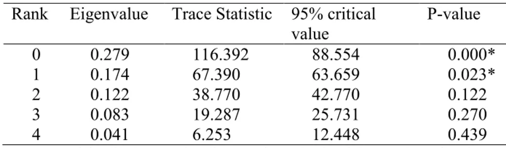
T is the coefficient matrix in front of the unrestricted coefficients. I use the Johansen procedure to specify the cointegrating vectors in the system. The Johansen trace test indicates two cointegrating vectors.
Rank Eigenvalue Trace Statistic 95% critical value
P-value
0 0.279 116.392 88.554 0.000*
1 0.174 67.390 63.659 0.023*
2 0.122 38.770 42.770 0.122
3 0.083 19.287 25.731 0.270
4 0.041 6.253 12.448 0.439
Note: Asterisks (*) denote, that the zero-hypothesis of the number of ranks can be rejected on a 5 % significance level. The tests start with the hypothesis that the rank of the matrix is ≤0 . The rank of the test is increased until the zero- hypothesis can be rejected.
Table 5. Johansen Trace test results
To identify the long run relations I normalize βଵ with regard to Prib and βଶ with regard to RM2. I test different possible variations of long-run relations for each ߚ-vector with an LR-test. The test reveals a money demand equation and an interest rate relation. The estimated and identified cointegrating vectors are summarized in Table 6. The cointegration space is identified with seven exclusion restrictions. The LM test does however not reject the thus overidentified model: ܺଶሺ5ሻ = 3.52432; − ݒ݈ܽݑ݁ = 0.61971 . The vector ߚመଵ represents the interest rate relation. The exchange rate and the price level are negatively related to the interest rate. The signs are plausible. The positive trend component indicates a low interest rate appreciation. ߚመଶ encompasses the real money demand equation. The real money demand increases almost proportionally to the RGDP (0.866). The negative dependence of the interest rate on real money demand is consistent with economic theory.
The approximate elasticity coefficient of 6.336 calculated from the monthly value on a yearly base (76.03229/12) is close to other results in the literature, ranging between 6.86 and 5.07 (Belke and Czudaj, 2010).
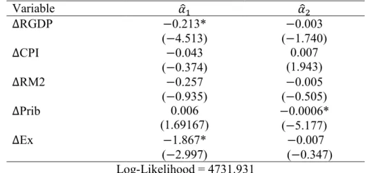
The deviations from the long-run interest rate and the money demand relation are only transitory and captured in ߝெ and ߝெ through the normalization on Prib and RM2 respectively. Money is neutral with this specification. The loading coefficients ߙො expose the dynamic of the endogenous variables for a temporary deviation from the long-run relations (Table 8). The estimation of the recursive eigenvalues (Figure 1) and 95% confidence intervals prove the stability of the parameters of the unrestricted VECM model with the two cointegrating vectors.
Variable ߚመଵ ߚመଶ
RGDP - −0.8660
(0.1170)
CPI 0.16703
(0.0303)
-
RM2 - 1
Prib 1 76.0323
(12.2448)
Ex 0.0292
(0.0109)
-
Trend −0.0002
(0.0000)
-
Note: is normalized to Prib to represent an interest rate relation. normalized to RM2 serves as a money demand equation. Standard deviations are in parenthesis.
Table 6.
Identified cointegration vectors in the VECM
The eigenvalues do not signal structural breaks in the estimated vectors of ࢼ and ࢻ.
Identification in the Structural VECM
The two cointegrating vectors imply the two transitory shocks. The remaining three ሺ݇ − ݎሻ shocks ߝௌ, ߝூௌ, and ߝா௫ have permanent effects on the dynamic of the system. The variables are ordered accordingly for the impulse response analysis x୲ = ሾRM2୲, Prib୲, Ex୲, RGDP୲, CPI୲ሿ. The first two columns of the impact matrix Ξ~are zero with this variable alignment and have no long-run effect. The additional restrictions distinguish the permanent shocks. The exchange rate shock does not influence output and prices in the long run. The demand shock is restricted to a neutral effect on output in the long run.
Ξ~ = ۏێ ێێ
ێۍ0 0 ߦெ,ா௫ ߦெ,ௌ ߦெ,ூௌ
0 0 ߦூ,ா௫ ߦூ,ௌ ߦூ,ூௌ
0 0 ߦா,ா௫ ߦா,ௌ ߦா,ூௌ
0 0 0 ߦ,ௌ 0 0 0 0 ߦగ,ௌ ߦగ,ூௌےۑۑۑۑې
The two transitory shocks differ in their contemporaneous effects set in the short-run impact matrix Ξ∗~. The monetary policy shock has a lagged effect on output, justified by the lagged response of real variables to nominal shocks. The shocks are orthogonalized through factorization of the estimated variance-covariance matrix with this identification.
બ~relies on a demanding numerical estimation technique (Lütkepohl Figure 1.
Timeline of the greatest recursive eigenvalues of the unrestricted VECM and its 95% confidence interval.
and Krätzig, 2004) while the maximum-likelihood method is used to estimate બ∗~.
Ξ∗~ = ۏێ ێێ
ێۍߦெ,ெ∗ ߦெ,ெ∗ ߦெ,ா௫∗ ߦெ,ௌ∗ ߦெ,ூௌ∗ ߦூ,ெ∗ ߦூ,ெ∗ ߦூ,ா௫∗ ߦூ,ௌ∗ ߦூ,ூௌ∗ ߦா,ெ∗ ߦா,ெ∗ ߦா,ா௫∗ ߦா,ௌ∗ ߦா,ூௌ∗ ߦ,ெ∗ 0 ߦ,ா௫∗ ߦ,ௌ∗ ߦ,ூௌ∗ ߦగ,ெ∗ ߦగ,ெ∗ ߦగ,ா௫∗ ߦగ,ௌ∗ ߦగ,ூௌ∗ ےۑۑۑۑې Results and interpretation
The identification of shocks enables the interpretation of the impulse responses. I analyze whether the responses are symmetric, which corresponds to the theoretical reactions predicted by the Mundell- Fleming-Dornbusch model. Then I compare the results to earlier studies to evaluate the changed transmission mechanism.
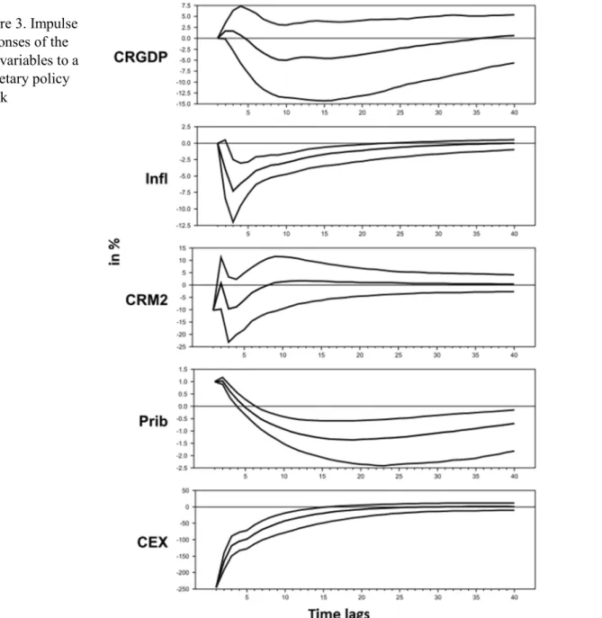
The recursive VAR and SVAR model are estimated by RATS.
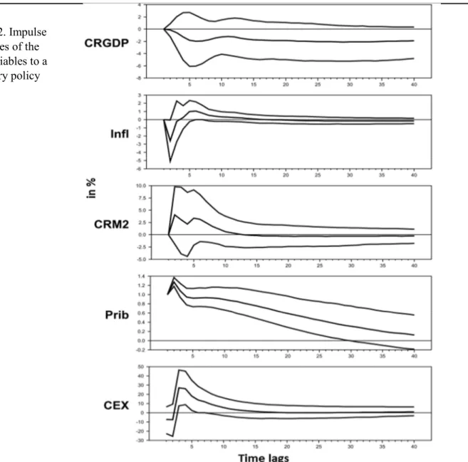
Figures 2 and 3 illustrate the responses of the variables over a 40- monthtime horizon to a 1% increase of the Prib (per month). The shock occurs only in the first period and imitates an increase of the per anno interest rate of 12.68 % which corresponds to an average increase of the interest rate of around 40 basis points. The uncertainty of the point estimations for the impulse responses are captured by the confidence bands of one standard deviation. Using a Monte Carlo simulation technique, I repeat the simulation 1000 times to calculate the confidence intervals. The impulse response functions are specified in percentage deviations from their initial level and refer to the transformed data.
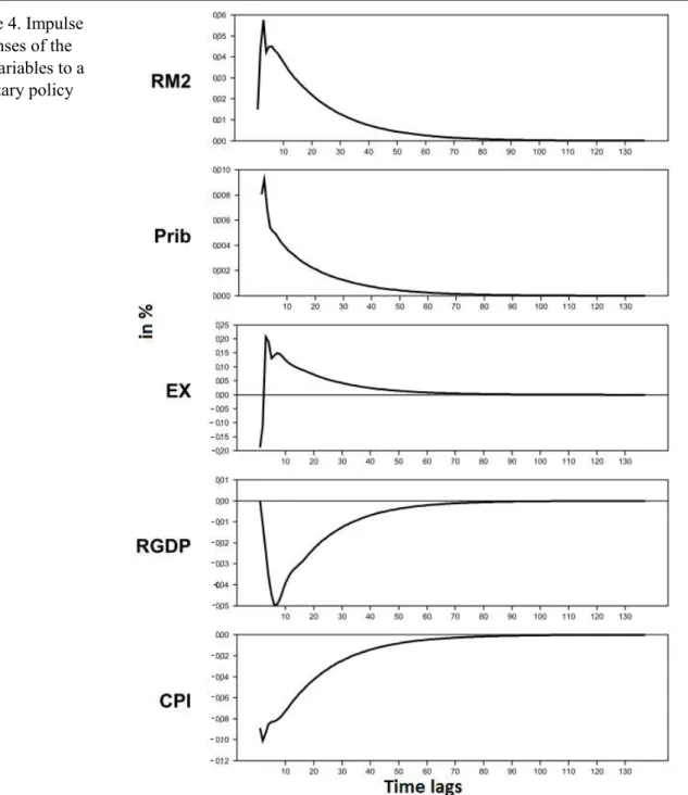
In the SVECM (Figure 4) I abstract from the confidence intervals because the theoretical characteristics of confidence bands in a non- stationary system are still not totally clarified (Lütkepohl and Krätzig, 2004). The problem is the singularity of the asymptotic distribution due to the possible zero variance. Zero variance can occur when the variables used for estimation are integrated. Therefore the significance of the impulse responses is not assessed for the SVECM. The time horizon on the x-axis spans over 10 years. The impulse responses of the variables are functions of their original log values which causes the scale difference. The magnitude of the shock differs in the SVECM due to technical reasons. The monetary policy shock of one standard deviation represents a change of the Prib of around one basis point. The qualitative
and quantitative interpretation are unaffected from these model differences.
Output falls by 2% in the VAR and 5% in the SVAR model at maximum in response to a positive interest rate shock. The reaction in the SVECM with 0.05% is proportional to the SVAR considering the different data format and shock degree. The bottom is reached after around 9 months. However, the confidence bands, when applied, do not state the significance of all reactions. The high uncertainty might be owed to the high fluctuations in the time series during the financial crisis.
Inflation drops significantly for around 3 months in the SVAR and insignificantly in the VAR model for around one quarter. In the SVECM the consumer price index decreases immediately after the shock. In no model is a price puzzle apparent. These reactions state an efficient pass through from the policy action to prices. The relatively quick reaction of the prices to monetary policy contraction might indicate that the Czech National Bank can successfully anchor inflation expectations.
The impulse responses of the real money supply show a liquidity puzzle in the recursive VAR and the SVECM. The real money supply, counterintuitively, increases after monetary tightening. The reaction in the VAR is less persistent than in the SVECM. The SVAR shows a significant drop of the real money supply only in the first months after the shock. That is in line with the theory since the demanded money supply decreases with an increase of the opportunity cost of money.
After monetary policy contraction, the uncovered interest parity condition implies an appreciation of the nominal exchange rate to compensate for the positive spread between the domestic and the foreign nominal interest rate as long as prices are rigid. The exchange rate gradually depreciates with the adjustment of prices. In the SVAR model this significant effect is observable. The extreme elasticity value of the exchange rate might be caused by the allowed simultaneity between the exchange rate and the interest rate in the SVAR. The recursive VAR and VECM show delayed overshooting. For two months after the shock, the exchange rate appreciates in the VAR and in the SVECM model. Then the rate overshoots its long-run level and gradually depreciates violating the interest rate parity condition (Dornbusch, 1976). In the long run in all models the exchange rate returns to the baseline. The magnitude of responses to Ex may to some extent reflect the general observation of high exchange rate volatility.
In the VAR, the SVAR, and the SVECM model, the variables’
reactions have generally the same sign but differ in their significance and quantitative effect. The SVAR model proved the pronounced reactions, while limited proportionality between the model specifications exists.
The responses in the VECM model are more persistent. A possible reason is that the model includes the original and differenced data and acknowledges long-run relations by cointegration. In conclusion, the sign effects of a monetary policy shock in the Czech Republic are robust to model specifications and are in line with the theory of the Mundell- Fleming-Dornbusch model.
Discussion of Results
Borys et al. (2009), among others, apply a recursive VAR and a SVAR with A-B restrictions for the time period from beginning of 1998 to mid 2006. The estimation is based on a stationary system with non-stationary time series. They also do not find evidence for a price puzzle as it is the case in the model Arnostova and Hurnik (2005), who estimate two recursive VAR models with different variable orderings. The reason for the price puzzle might be the examination period, which spansfrom 1994 to 2004 and includes regime shifts (Egert and MacDonald, 2009).
Compared to other studies, the results in this paper state a rapid reaction of prices to the monetary policy action. That suggests that prices have become more responsive to monetary policy shocks, reflecting an effective pass-through. The deepening of the financial sector and the banking system might have facilitated this development.
Comparable studies for the Czech Republic include the nominal money supply instead of the real money supply which I choose here to comply to the money demand interrelations in the Mundell-Fleming- Dornbusch model. Anzuini and Levy (2007) state that the exclusion of the money aggregate does not change the results. In their recursive and structural VAR model money’s reaction is likewise insignificant. The money supply evolved almost parallel to the real GDP over the time horizon. Likewise the financial crisis might have caused the unclear results.
The incongruent reaction of the nominal exchange rate of the models conforms to earlier studies. Borys et al. (2009) also find delayed overshooting in their model. Arnostova and Hurnik (2005) find evidence for an exchange-rate puzzle by depreciation of the exchange rate after the contractionary shock. In particular, in the SVAR model the strong
response of the exchange rate indicates high exchange-rate volatility connected with monetary policy actions. To some extent the effect is reasonable for a small open economy because of the structural appreciation of the domestic currency with the catching-up process and the general nation’s export orientation.
Monetary policy affects the economy close to what theory predicts, which earlier studies could not provide due to regime shifts. The effects are partially symmetric to the observed transmission mechanisms in countries of the Eurozone (Weber et al., 2009; Peersman and Smets, 2001).
Conclusion
In the Czech Republic, the transition to an inflation targeting and floating exchange rate regime has changed the monetary transmission mechanisms. This paper analyzes the effects of a contractionary monetary policy shock with a recursive VAR, SVAR, and a SVECM model over a time period that consists of a uniform regime. The data set includes the minimal variable set necessary for the analysis to reduce statistical inference. The restrictions used to identify the shocks are based on the Mundell-Fleming-Dornbusch model and the assumption of money neutrality by accounting for long-run relations.
The model estimation documents the following results: Prices and output decrease after monetary tightening. The inflation rate is very responsive and returns faster back to the steady state level than does output. The reaction of the output variable is, however, connected with a high degree of uncertainty. The real money supply increases insignificantly, which is puzzling. The mixed exchange rate reactions point to high exchange-rate volatility. The reaction in the recursive VAR and SVECM model exhibit delayed overshooting. Besides the liquidity puzzle, monetary policy affects the economy as predicted by the Mundell-Fleming-Dornbusch model.
The sign effects of the variables following a monetary policy shock are identical over all model specifications, indicating robust results. The dynamic of the variables in the VECM are more persistent likely caused by the use of level variables.
The quick response of prices compared to output suggests that the Czech National Bank is credible in pursuing its objective of price stability. This study provides no evidence for a price puzzle that resulted
in comparable earlier studies. The outcome confirms that estimation over a time period with a single regime solves the paradox reaction of prices.
The credit channel of monetary transmission has gained unprecedented relevancy following the recent financial crisis. The inclusion of credit aggregates in the VAR estimation would allow evaluating the pass- through from a key interest rate increase over the credit market to the real economy and prices. I leave this idea for future research. The analysis provided evidence for an efficient inflation targeting of the Czech Republic through a functional pass-through from money interest rate to prices.
References
Anzuini, A., & Levy, A. (2007). The monetary transmission mechanism in the Czech Republic. Applied Economics, 39(2007), 1147-1161 Arnostova, K., & Hurnik, J. (2005, December). The monetary
tranmission mechanism in the Czech Republic (Evidence from VAR analysis). CNB Working Paper Series no.4, Czech National Bank.
Artis, M., & Ehrmann, M. (2006). The exchange rate - A shock-absorber or a source of shocks? A study of four open economies Journal of International Money and Finance, 25(6), 874-893
Belke, A., & Czudaj, R. (2010). Is Euro area money demand (still) stable? Cointegrated VAR versus single equation techniques. Ruhr Economic Papers no. 171.
Bernanke, B., & Mihov, I. (1998). The liquidity effect and long-run neutrality. Carnegie-Rochester Conference Series on Public Policy, 49(December), 149-194
Bjornland, H. (2008). Monetary policy and exchange rate interactions in a small open economy. The Scandinavian Journal of Economics, 110(1), 197-221
Blanchard, O., & Quah, D. (1989). The dynamic effects of aggregate demand and supply disturbances. The American Economic Review, 79(4), 655-673
Borys, M. M., Horvath, R., & Franta, M. (2009). The effect of monetary policy in the Czech Republic: an Empirical Study. Empirica, 36(4), 419-443
Coricelli, F., Egert, B., & MacDonald, R. (2006). Monetary transmission mechanism in Central and Eastern Europe: Gliding on a wind of change. Working Paper No. 850, William Davidson Institute.
Creel, J., & Levasseur, S. (2005). Monetary policy transmission mechanism in the CEECs: How important are the differences with the Euro Area. Observatoire Francais des Conjonctures Economiques no. 2005-02
Czech National Bank. (2012). Nominal Exchange Rate. Retrieved June
2012, from CNB Code:10916:
http://www.cnb.cz/docs/ARADY/HTML/index_en.htm
Czech National Bank. (2012). Time series of the 3-months Pribor.
Retrieved June 2012, from CNB Code 85/1064:
http://www.cnb.cz/docs/ARADY/HTML/index_en.htm
Dornbusch, R. (1976). Expectations and exchange rate dynamics.
Journal of Political Economy, 84(6), 1161-1176.
Egert, B., & MacDonald, R. (2009). Monetary Transmission Mechanism in Central and Eastern Europe: Surveying the Surveyable. Journal of Economic Surveys, 23(2), 277-327.
Endres, W. (2010). Applied Econometric Time Series. USA: John Wiles and Sons, Inc.
Gali, J. 1992. How well does the IS-LM model fit Postwar U. S. Data?
The Quarterly Journal of Economics, 107(2),May
Ganev, G., Molnar, K., Rybinski, K., & Wozniak, P. (2002).
Transmission mechanism of monetary policy in Central and Eastern Europe. Network Reports 52, Center for Social and Economic Research.
Juselius, K. (2009). RATS Handbook: The cointegrated VAR Model.
Estima Part I, November 2009.
King, R., & Watson, M. W. (1997). Testing Long Run Neutrality.
Working Paper Series 4156, National Bureau of Economic Research.
Lastrapes, W. 1998. International evidence on equity prices, interest rate and money. Journal of International Finance, 17(3), 377-406.
Lütkepohl, H. (2005). New Introduction to multiple time series analysis.
Berlin, Heidelberg: Springer-Verlag.
Lütkepohl, H., & Krätzig, M. (2004). Applied Time Series Econometrics.
Cambridge: Cambridge University Press.
Main Economic Indicators, OECD. (2012). Time series of the nominal money aggregate M2 in the Czech Republic. Retrieved from Thomson Datastream Code 870000874.
Main Economic Indicators, OECD. (2012). Time series of total Consumer Prices in the Czech Republic. Retrieved from Thomson Datastream Code 870000856.
Mitra, P., Zalduendo, J., & Selowsky, M. (2010). Turmoil at Twenty - recession, Recovery, and the Reform in Central and Eastern Europe and the former Soviet Union. Washington DC: The international Bank for Reconstruction and Development/The World Bank.
Oxford Economics (2012). Time series of the Czech Gross Domestiv Product. Retrieved from Thomson Datastream Code CZXGDPR.D.
Peersman, G., & Smets, F. (2001). The monetary transmission mechanism in the Euro Area: More Evidence from VAR Analysis.
Working Paper 91, European Central Bank.
Reade, J. (2005). The cointegrated VAR methodology. Summer School in Econometrics at the University of Copenhagen.
Sims, C. (1986). Are forecasting models usable for policy analysis?
Federal Reserve Bank of Minneapolis Quarterly Review, 10(1), 2-16 Sims, C. A. (1980). Macroeconomics and Reality. Econometrica, 48(1),
1-48
Weber, A., Gerke, R., & Worms, A. (2009). Has the monetary transmission process in the Euro area changed? Evidence based on VAR estimates. Working Paper No. 276, BIS.
Appendixes
Variable ߙොଵ ߙොଶ
ΔRGDP −0.213*
(−4.513)
−0.003 (−1.740)
ΔCPI −0.043
(−0.374)
0.007 (1.943)
ΔRM2 −0.257
(−0.935)
−0.005 (−0.505)
ΔPrib 0.006
(1.69167)
−0.0006*
(−5.177)
ΔEx −1.867*
(−2.997)
−0.007 (−0.347) Log-Likelihood = 4731.931
Asterisks (*) denote the loading coefficients that are significant on 5 % significance level. T-values are in parentheses.
Variable Describtion and Source
RGDP Quarterly seasonally adjusted real GDP, based on a price index with the reference year 2005, in million aof Czech korona (Oxford Economics , 2012)
CPI Log difference of the monthly non-adjusted consumer price index, (Main Economic Indicators, OECD, 2012) RM2 Non-adjusted nominal money aggregate M2 (Main
Economic Indicators, OECD, 2012)
Prib The Pribor is a p.a. interest rate is calculated to a monthly base; used as a gross interest rate (Czech National Bank, 2012)
Ex Nominal exchange rate between the Czech Koruna and the Euro. Direct quotation, not seasonally-adjusted (Czech National Bank, 2012)
Table 7. Data describtion and sources
Table 8. Loading coefficients of the VECM.
Estimation is based on the recursive VAR. Deviations from the baseline are in percent over a 40-month period. Confidence bands of one standard deviation are simulated by the Monte Carlo method.
Figure 2. Impulse responses of the five variables to a monetary policy shock.
Estimation is based on the SVAR. Deviations from the baseline are in percent over a 40-month period. Confidence bands of one standard deviation are simulated by the Monte Carlo method.
Figure 3. Impulse responses of the five variables to a monetary policy shock
Estimation is based on the SVECM. Deviations from the baseline are in percent over a 140-month period.
Figure 4. Impulse responses of the five variables to a monetary policy shock
Figure 5. Original logged time series of the Czech real GDP, CPI, real M2, the Pribor, and the exchange rate of the Czech Koruna and the Euro from January 1999 to
September 2011.
Figure 6.
Transformed time series of the Czech real GDP, CPI, real M2, and the exchange rate of the Czech Koruna and the Euro from January 1999 to
September 2011.