Research Collection
Working Paper
A dynamic approach to car availability throughout the life course
Author(s):
Crastes dit Sourd, Romain; Dubernet, Ilka; Beck, Matthew; Hess, Stephane; Axhausen, Kay W.; Holz-Rau, Christian; Scheiner, Joachim
Publication Date:
2020-08-26 Permanent Link:
https://doi.org/10.3929/ethz-b-000438685
Rights / License:
In Copyright - Non-Commercial Use Permitted
This page was generated automatically upon download from the ETH Zurich Research Collection. For more information please consult the Terms of use.
ETH Library
course
Romain Crastes dit Sourd Ilka Dubernet Matthew Beck Stephane Hess Kay W. Axhausen Christian Holz-Rau
Joachim Scheiner August 26, 2020
WORKING PAPER - DO NOT QUOTE WITHOUT PERMISSION.
Abstract
The relatively new research field of mobility biographies designates the analysis of long-term mobility behaviour and the availability of mobility tools in a life span. A retrospective survey of the TU Dortmund, ETH Zurich and Goethe University Frank- furt collects data on individual mobility biographies of three different generations in a household with a life-calendar. Most of the past long-term decisions made by in- dividuals such as buying a house or changing job affect their preferences in future periods and induce economic constraints in the form of transaction costs. Ignoring these aspects may lead to biased estimates in the analysis. A dynamic probit model is used to identify impacts on the individual decisions on car availability in a life span and tests for differences between gender or is used to include the time dependency of the explanatory variables such as age, the number of children or education. The focus of the paper is to compare the modelling results following common practices in the life course calendar literature, based on random effects probit models with the results obtained with a dynamic random effects probit model with autocorrelation.
In contrary to the classic random effects probit model approach the main advantage of the dynamic probit approach is to explicitly model the correlated time-fixed and time-varying unobserved heterogeneity by the means of composite marginal likelihood estimation.
Keywords: car availability, life course analysis, composite marginal likelihood, mo- bility biography
1 Introduction and related work
The contemporary increasing complexity of household and family structures, labour mar- kets changes and individualisation of lifestyles cohere with an increase in activities and flexibility, changing attitudes and behaviour patterns. This also affects individual mo- bility behaviour as well as mobility tool ownership. It is still challenging to capture such
1
ideas conceptually, methodically and empirically, and to identify the most influential factors in order to contribute to planning practice (Axhausen, 2008). So far changes in mobility behaviour are often covered with static cross-sectional studies but these neglect the dynamic and implications of long term decisions (Lanzendorf,2003).
In the past decade the focus of interest therefore shifted towards individual and joint long term decisions in a life span. The biography approach examines mobility behaviour (including residential choice and travel behaviour) in the context of key events in a life course (such as changes of job or family formation) and life phases (e.g. adolescence or the family phase). Besides people’s own experiences the influence of the social environ- ment is of interest. The relevance of both the life course and the social environment are acknowledged in the theoretical discussions about mobility biography and mobility socialisation (Scheiner,2007). Beige and Axhausen(2012) show that strong interdepen- dencies exist between the various key events and long-term mobility decisions during the life course and argue that events occur to a great extent simultaneously.
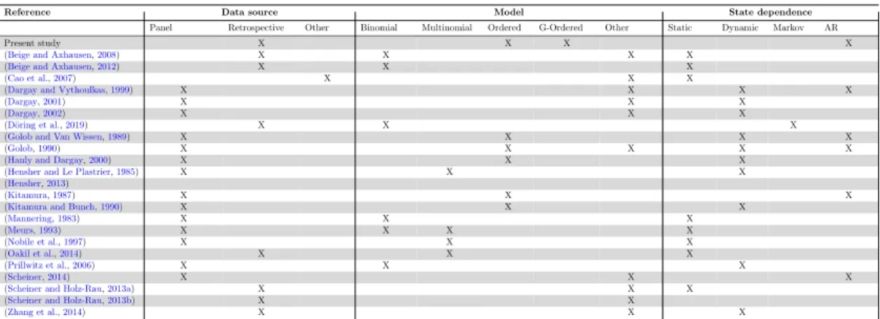
Several empirical studies reported in Table 1 attempt to understand and explain everyday travel behaviour as a routine activity changing due to key events such as resi- dential relocation, the birth of a child or exogenous interventions. The different studies are classified based on the data source they use, the type of model they propose (un- orderedversus orderedversus continuous), as well as how the influence of past outcomes (the dynamic process) is accounted for in the model. In a large majority of cases, we find that the work based on retrospective data is not accounting for the dynamic nature of the mobility decisions made throughout the life course. A similar conclusion is shared by a comprehensive review of the theoretical framework and most important studies in- vestigating mobility behaviour and mobility tool ownership over the life course recently published by M¨uggenburg et al. (2015). The authors address open research questions and conclude that studies often investigate long-term decisions with static (panel) mod- els and neglect the dynamic, causality, interrelations and time dependency of the target and explanatory variable (M¨uggenburg et al.,2015). In addition, most econometric ap- plications hypothesise that car availability (or car ownership) should be modelled as a series of discrete choices following the findings from Bhat and Pulugurta (1998) while recent findings from the qualitative literature indicate that ”car ownership changes are more seen as a process rather than as discrete decisions” (Clark et al.,2016).
This paper addresses these shortcomings by proposing an autoregressive generalised ordered probit model for modelling car availability, thus taking the earlier described de- pendencies into account while also engaging with findings from the qualitative literature by representing car availability as a process driven by a single latent variable rather than a choice between several alternatives. Section2discusses the factors that have driven car ownership and car availability to be mainly modelled as a succession of discrete choices and proposes an alternative framework. Section3further describes the framework of the model, which is subsequently applied to empirical data of a retrospective survey. The paper continues with the description of the data set used for the application in theData
Table 1: Overview on (quantitative) studies on car availability & ownership
Reference Data source Model State dependence
Panel Retrospective Other Binomial Multinomial Ordered G-Ordered Other Static Dynamic Markov AR
Present study X X X X
(Beige and Axhausen,2008) X X X X
(Beige and Axhausen,2012) X X X
(Cao et al.,2007) X X X
(Dargay and Vythoulkas,1999) X X X X
(Dargay,2001) X X X
(Dargay,2002) X X X
(D¨oring et al.,2019) X X X
(Golob and Van Wissen,1989) X X X X
(Golob,1990) X X X X X
(Hanly and Dargay,2000) X X X
(Hensher and Le Plastrier,1985) X X X
(Hensher,2013)
(Kitamura,1987) X X X
(Kitamura and Bunch,1990) X X X
(Mannering,1983) X X X
(Meurs,1993) X X X X
(Nobile et al.,1997) X X X
(Oakil et al.,2014) X X X
(Prillwitz et al.,2006) X X X
(Scheiner,2014) X X X
(Scheiner and Holz-Rau,2013a) X X X
(Scheiner and Holz-Rau,2013b) X X
(Zhang et al.,2014) X X X
description Section (4). The model results are presented and discussed in the Results Section (5). Section 6, Conclusions and Outlook, summarizes this paper and gives an outlook on future work and challenges.
2 Ordered and unordered response structures for mod- elling car availability
In this section, we address a fundamental question which has receive extensive attention in the literature on car ownership and which relates to whether vehicle ownership should be modelled by the means of an ordered or unordered-response mechanism. In a partic- ularly influential paper, Bhat and Pulugurta (1998) present the underlying theoretical structures and identifies the advantages and disadvantages of the two response mech- anisms. The unordered response system approach is based on a utility maximisation hypothesis while the ordered response system approach assumes that a single continuous variable represents the latent car ownership propensity of an agent (a household or an individual for example). The authors point out that the unordered response system, which is represented by the well-known multinomial logit model (MNL), is better at capturing a pattern of elasticity effects of variables across alternatives, while the ordered response system, represented by the ordered logit model (OL), is”constrained to have a more rigid trend in elasticity effects”.
More precisely, the econometric framework for modelling car ownership via a MNL structure can be defined as follows: let the utility of car ownership levelkbe a function of a vector of exogenous variables xassociated with an agentibe written as:
Uk,i=β0kxi+k,i (1)
where βk is a vector of parameters (including a constant) to be estimated for each
car ownership level with k = 1,2,...K. For identification reasons, the parameters for one of the car ownership levels must be normalised to zero. In the notation which we adopt and which is used for modelling car availability rather than car ownership in the remainder of this paper, all the exogenous variables in the model are associated with agent characteristics as opposed to car features. Following the usual assumption about the error term being independently and identically distributed across alternative car ownership levels and following a Gumbel distribution, the choice probability for agent i to choose car ownership levelk corresponds to:
Pk,i= eβ0kxi Pk0=K
k0=0 eβk0xi (2)
In contrast, the econometric framework for the ordered response structure, which in this paper will consist in an ordered probit, is defined as follows:
y∗i =β0xi+i, (3)
wherey∗i is an unobserved latent process related tocar availability propensity defined as a function of relevant exogenous variables. iis an index for individuals xi is a vector of exogenous variables, andβ0 is a vector of coefficients to be estimated. The error termi
is assumed to follow a standard normal distribution with zero mean and unit variance (changing this assumption to a Gumbel distribution leads to the OL model used byBhat and Pulugurta(1998)). The discrete outcome observed for individualistill corresponds to ki, where ki may take one value among K. However, we now have that yi = ki if µk−1,i < yi∗ < µk,i, where µk,i is the upper bound threshold corresponding to the discrete levelki withµ0 =−∞andµK = +∞. With this notation,µ1,µ2, ...,µK−1 are parameters to be estimated withµ1 < µ2 < ... < µK−1. The probability for observing a given outcomek for agentiis now given by:
Pk,i= Φ(µk,i−β0xi)−Φ(µk−1,i−β0xi) (4) where Φ stands for the standard normal cumulative distribution. The ordered structure contrasts with the unordered response structure which features one (latent) utility for each potential outcome, instead of one single latent process related to car availability.
This important distinction makes the ordered choice model closer to the findings of Clark et al. (2016), who state that ”household car ownership level should be considered as the outcome of a continuous process of development over the life course, rather than as discrete decisions”. However, this does not necessary mean that ordered model structures have been found to be a superior alternative to model car ownership decisions.
Indeed, using four different datasets, Bhat and Pulugurta(1998) estimate a series of models and compare the relative performances of the ordered and unordered response
structure by looking at measures of fit in an estimation and a validation sample. Their comparative analysis offers evidence that ”auto ownership modelling must be pursued using the unordered-response class of models”. However, this is mainly driven by the fact that an unordered model will feature K-1 times more parameters than an ordered model all else being equal. More recent papers have introduced a more flexible class of ordered response structure models known as generalised or hierarchical ordered response models. Such class of models has been originally proposed by Maddala (1986), Ierza (1985) and Srinivasan (2002) with further refinements proposed byEluru et al. (2008), among others.
2.1 Generalised ordered structures
Generalised ordered response structure models are built on the same principles as the simple ordered structure previously described (which means that such models still feature K−1 thresholds), but allow the thresholdsmuto vary across agents based on observed or unobserved heterogeneity. In this paper, we are particularly interested in the structure where thresholds are a function of exogenous variables related to the characteristics of the agents, labelledzand which is not restricted to the variables featured inx although this is the case in our application. A similar model is proposed byEluru (2013) and we adopt an analogous notation:
µk,i=µk−1,i+eκk+ζk0zi (5)
For identification reasons, one of the thresholds must remain constant across agents, meaning that µk,i =µk−1,i+eκk. The choice of which threshold to set as the base (or reference) is arbitrary. Assuming a (standard) normally distributed error term for the unobserved latent outcomeY∗ leads to the generalised ordered probit model, for which the likelihood function simply corresponds to Equation8. In the literature, several studies have compared the generalised ordered response structure with an unordered response structure (Eluru, 2013). The generalised ordered response structure, by allowing more flexible thresholds than classic ordered response models, is found to be on par with the unordered response structure, which is mainly driven by the fact that such specifications can now feature the exact same number of parameters all else being equal. The choice of an ordered or unordered specification should hence be made based on whether researchers seek to explicitly recognise the inherent ordering within the decision variable or not, as well as whether no major discrepancies can be reported in terms of goodness-of-fit between a generalised ordered response structure and an equivalent unordered model.
Having clarified the fact that an unordered response model should not be considered asa priori superior to an ordered response structure for modelling car availability and having demonstrated the compatibility of this approach with the qualitative findings of Clark et al. (2016), we now move on to the description of panel generalised ordered response structures for large time series, which are typically encountered in mobility biography studies.
3 Modelling work
3.1 Panel probit
The panel generalised ordered probit model simply consists in introducing a random effect in the cross-sectional generalised ordered model previously introduced. Thelatent car availability propensity for an agent iis given by:
y∗ij =β0xij +αi+ij, (6)
wherejis an index for thejth observation for agenti, withj= 1, 2, ...,J the number of periods under study, xij is a vector of exogenous variables which can vary across time, and β0 is a vector of coefficients to be estimated. The new parameter, αi, corresponds to an individual specific random disturbance (i.e. a random effect). Finally, the serially independent error termij is assumed to follow a standard normal distribution with zero mean and unit variance.
The discrete outcome observed for individual i at time j corresponds to kij, where kij may take one value among K at each time period (kij = 1, 2, ..., K). In the context of this paper, kij refers to a given level of car availability among K (”never available”, ”sometimes available” or ”always available”). We have again thatyij = kij
if µijk−1 < yij∗ < µijk, where µijk is the upper bound threshold corresponding to the discrete levelkij with µ0 =−∞ and µK = +∞. We have again that the thresholds are allowed to vary based on observed characteristics of the agents or their environment:
µk,ij =µk−1,ij+eζk+βk0xij (7)
Finally, αi = α + ηi where ηi is an individual-specific random term. The role of ηi is to generate an equi-correlation between the repeated choice situations for a given individual. The α parameter is normalised to 0 if µ1 is estimated (and the reverse is also possible). In this paper, we consider that ηi is normally distributed with variance σ2 but other distributional assumptions may be tested. The model is easily and rapidly estimated using Maximum Simulated Likelihood (MSL). The probability of the observed vector ki of the sequence of ordinal choices (ki1, ki2, ..., kiJ) for individual i given the individual specific random term ηi can be written as:
P(ki)|ηi=
J
Y
j=1
Φ(µijk−α−β0Xijk−1−ηi)−Φ(µij −α−β0Xij −ηi)
(8) where Φ stands for the standard normal cumulative distribution. It is then easy to integrate out the individual specific random-termηi in order to obtain the unconditional
log-likelihood of the observed choice sequence.
logLi(θ) = log
Z +∞
−∞
J
Y
j=1
Φ(µijk−α−β0Xij−σv)−Φ(µijk−1−α−β0Xij −σv)
φ(v)dv (9)
where v = ησi with ηq ∼N(0, σ2) and θ corresponds to a vector of parameters. The log-likelihood function of the P-GOPROBIT entails only a one dimensional integral so model estimation is generally fast.
3.2 Autoregressive structures
The simple model presented above assumes that the multiple observations for each in- dividual are equally correlated across time. However, we seek to model car availability as a dynamic process, that is to account for the fact that Y∗ is influenced by its past realisations. From a behavioural point of view, this means that we assume that some of the unobserved factors affecting car availability at time t are correlated with the same unobserved factors at timet−1,−2,−T, giving rise to an autoregressive process.
We argue that such a modelling approach is necessary to better explaincar availability changes over time as a process (Clark et al., 2016) in the sense that it better captures the temporal dimension of such process.
We follow Paleti and Bhat (2013) and assume a classic autoregressive structure of order 1 (AR1). We define corr(ij, ig = ρ|tij−tig|) with tij the measurement time for observation yij (g 6=j), where 0 < ρ < 1, a constraint that be easily enforced through a logistic transformation. The latent outcomes y∗ij now follow a multivariate normal distribution for the ith individual. The mean vector of the multivariate normal distri- bution may be standardised in which case it corresponds to α+βτ0Xi1,α+βτ0Xi2, ...,α+βτ0XiJ while the correlation matrix Σ has non diagonal entries ζig = σ2+ρ
|tij−tig|
τ2 , where τ, the standard deviation of the latent outcome y∗ij, corresponds to √
σ2+ 1. While (9) only entails a one-dimension integral, the autoregressive model requires the evaluation of an integral of dimensionJ for agenti. The log-likelihood function becomes:
logLi(θ) =
Z δmi1
w1=δmi1−1
, ..., Z δmiJ
wJ=δmiJ−1
φJ(w1, ..., wJ|Σ)dw1, ..., dwJ
, (10)
where δmij = µmij−α−βτ 0Xij and φJ is the standard multivariate normal distribution of dimensionJ and w1, w2, ..., wJ are the normalised means.
The dimensionality of integration often rules out the use of MSL for estimating the autoregressive panel generalised ordered probit model. For example, in the context of
the application presented in this paper, such a model would take weeks if not months to converge and would be very prone to simulation errors (Paleti and Bhat,2013). These issues are easily circumvented by the Composite Marginal Likelihood (CML) estimation approach, which, in the context of this paper, entails only the evaluation of pairs of bivariate normal probabilities.
3.3 Composite Marginal Likelihood estimation
Recently, the Composite Marginal Likelihood (CML) and its developments such as the Maximum Approximate Composite Marginal Likelihood (MACML) methods have be- come popular alternatives to MSL in the choice modelling field (Bhat,2011;Varin,2008;
Varin and Czado,2009;Varin et al.,2011). Composite Likelihood is an inference function derived by multiplying a collection of component likelihoods, where the collection used is determined by the context (Varin et al.,2011), and where each individual component is a conditional or marginal density, leading to an unbiased estimator. Paleti and Bhat (2013) simply describe CML as an estimation technique which replaces the multivariate probability of the dependent choices in the likelihood function by a compounding of prob- abilities of lower dimensions. A growing literature on CML estimation has proven that this estimation technique can perform as well as MSL at a fraction of the computational cost (Paleti and Bhat, 2013). It is worth noting that there exists a Bayesian approach to CML estimation (Pauli et al.,2011).
3.4 The composite marginal likelihood autoregressive panel ordered probit model
The CML functions presented in this paper are pairwise-likelihood functions formed by the product of likelihood contributions of varying subsets of pairs of observed events.
The following equation assumes that all the possible pairs are used for each individual.
A typical full-pairwise log-likelihood function for theith individual corresponds to:
logLi(θ) =
J
X
g=j+1 J−1
X
j=1
wi·log
P r(yij =kij, yig =kig)
, (11)
where wi is a weight which varies across individuals in unbalanced panel data contexts and
P r(yij =kij, yig =kig)
=φ2(δkij, δkig, ζig)−φ2(δkij, δkig−1, ζig)
−φ2(δkij−1, δkig, ζig) +φ2(δkij−1, δkig−1, ζig)
(12)
It is worth noting that (12) can be evaluated rapidly by using the rectangle properties of the bivariate normal distribution. Varin and Czado (2009) indicate that the CML estimator is consistent and asymptotically normally distributed, where the asymptotic
variance covariance matrix is given by the Godambe sandwich information matrix (Go- dambe,1960;Zhao and Joe,2005). The CML formulation is remarkably short and simple in comparison to its MSL counterpart. However,Paleti and Bhat(2013) as well asVarin and Czado (2009), among others, have proved that it is as able as the MSL approach to estimate the model parameters while being less prone to convergence issues. It is important to mention that although 11 uses all possible pairs of observations for each individual. However, the whole set of pairs for each individual may not be necessarily used in practice.
3.5 Model composition
The full-pairwise marginal likelihood function also presented in equation (11) requires the evaluation of J ×(J −1)/2 pairs of bivariate normal probabilities in the case of J time periods observed for each individual in the dataset. A full-pairwise approach is efficient and computationally affordable when the number of time periods is moderate, where the definition of moderate depends on the context and the sample size, amongst other factors. The full-pairwise approach becomes more computationally intensive as the number of time periods increases. A recent stream of studies proved that there may be no need to make use of all possible pairs, as pairs formed from closer observations provide more information than distant pairs. This has been found to be true in both temporal and spatial contexts (Bhat et al.,2014;Varin and Vidoni,2005). Bhat et al.(2014) suggests that the optimal maximum distance d between pairs can correspond to the value that minimises the trace (or the determinant) of the asymptotic variance-covariance matrix of a model with as complete a specification of covariate effects as possible. A similar proposition has been made by Varin and Vidoni (2005). Bhat et al. (2014) and Varin and Vidoni (2005) simply suggest starting with a low value of the distance threshold (which requires the evaluation of a small number of pairs in the CML function) and increase the distance threshold up to a point where increasing it does not improve the trace, or even increases it. Formally, this approach can be defined as the weighted sum of the log-bivariate densities of pairs of observations that are distant apart up to lagd.
In this paper, we build our model by following this approach.
Finally, in the context of unbalanced panel data, that is when the number of obser- vations for each individual varies across the sample, it is necessary for CML estimation to be efficient to vary the weight factorwacross respondents. In their review,Paleti and Bhat(2013) report a number of weighting strategies and in particular the recent contri- bution from Joe and Lee (2009), who suggest to setwq = (Ji−1)−1[1 + 0.5(Ji−1)]−1. In this paper, we follow the recommendations from Joe and Lee (2009) given that the panel we use is unbalanced, as introduced in the next section.
4 Data description
The data originates from a retrospective survey which is carried out since 2007 at a the Department of Transport Planning of the TU Dortmund as an annual first-year seminar’s homework. The questionnaire for the survey was primarily designed as part of a diploma thesis (Kl¨opper and Weber,2007) and has been used since then without adjustments to guarantee the comparability of the data. Since 2012 it is part of the collaborative project
”Mobility Biographies: A Life-Course Approach to Travel Behaviour and Residential Choice” and data is additionally collected in Frankfurt and Zurich.
The survey addresses the students of the seminar, their parents and grandparents.
The students represent the seeds and are asked to give the questionnaire to both their parents and two of their grandparents - who are randomly chosen, one from the maternal and one from the paternal side. If one of the family members is not available for any reason the students can alternatively ask another person preferably of the same gener- ation. The questionnaire which is the same for every generation asks for retrospective information on an individual’s residential and employment biography, travel behaviour and holiday trips as well as socio-economic characteristics and behavioural attitudes.
From 2007 - 2012 the participation in the survey was mandatory for the students in Dortmund which hence resulted in an average response rate above 90%. In 2013 the students could participate voluntarily thus the rate dropped to almost 20% which is slightly higher but still comparable to the response rates experienced in Frankfurt and Zurich in 2013 where participation was also voluntary. Consequently since 2014 the data collection is again mandatory in Dortmund and also in Frankfurt. Due to university ethical guidelines participation in Zurich remains voluntary. The data is collected at a person level so that every individual represents one case in the dataset. It is also possible to identify the members of one family and model aggregated groups.
4.1 Data issues
As the sample has a unique structure it is not possible to appraise representativeness (see (Erickson, 1979) for problems with representativeness in snowball surveys). The seeds are participants of a university seminar thus due to survey design highly educated individuals are likely to be overrepresented in all three generations. The majority of the respondents live in Dortmund respectively North Rhine-Westphalia - one of the most densely populated regions of Germany - so the data might also contain a bias to a more urban population. Furthermore within the grandparent generation a bias to female participants who live longer on the one hand and are also often younger, more popular and communicative can be recognized (Scheiner et al.,2014). Finally retrospective data especially collected for a long period as the life course always bears the risk of the so called memory bias which means a unintended or voluntary bias of the autobiographic memory (Manzoni et al.,2010). However the whole study focusses on mobility behaviour in the life-course and on finding intergenerational relations thus the results are not expected
to be significantly affected by the structural differences between the sample and the population. A more detailed documentation of the data set can be found in Scheiner et al. (2014)
4.2 Survey sample
For this paper data gathered for the parents generation in Dortmund from 2007-2012 is analysed. The dataset contains 684 respondents. The minimum age is 18 years old while the maximum is 72. One observation correspond to one year for a given respondent.
The data set features 20044 observations in total, meaning that it is unbalanced. The maximum number of observation for a respondent is 51. The variables which are used for modelling car availability in the remainder of the paper are introduced below:
Car availability (Categorical dependent variable): whether a car is0 - Never avail- able,1 - Sometimes available or2 - Always available.
age: age in years
distw: distance to work, in kilometers
german: 1 if the nationality of the respondent is german, 0 else
own home: 1 if the respondent owns its home, 0 else
moped: 1 if the respondent owns a moped, 0 else
moving: 1 if the respondent changed home on a given year, 0 else
children: Number of children
birth: 1 if birth of a child on a given year, 0 else
married: 1 if the respondent is married, 0 else
wed: 1 if year of wedding, 0 else
licence moped: 1 if the respondent has a license for driving a moped, 0 else
licence car: 1 if the respondent has a license for driving a car, 0 else
central 1 t0 5: whether the respondent lives in a central location or not. 1 if the respondent corresponds to the given category, 0 else. Ranges from very central (central1) to very remote (central5)
pop 1 to 7: whether the respondent lives in a large city of not. 1 if the respondent corresponds to the given category, 0 else. Ranges from less than 1,000 inhabitants (population1) to more than 500,000 inhabitants (population7)
edu cat: Types of education. 1 if the respondent corresponds to the given category, 0 else.
degree: 1 if the respondent has a degree and 0 else
home cat: Type of home. 1 if the respondent corresponds to the given category, 0 else.
In addition, we provide more details about the distribution of car availability across time in Figure1below:
Figure 1: Car availability across time
4.3 Modelling strategy
The objective of this modelling work is to model car availability as a dynamic process rather than a series of decisions over time, which calls for using an ordered response structure model while also accounting for the panel nature of the data and autocorrelation in the errors. However, a series of conditions need to be fulfilled before estimating such a model. Firstly, it is necessary to control whether there is an important discrepancy in terms of goodness-of-fit between an ordered and unordered response structure for modellingcar availability. Secondly, the impact of accounting for the dynamic nature of the process by modelling autocorrelation in the errors needs to be carefully assessed by
also estimating a non-dynamic model and comparing results. Finally, the model outputs need to be reported as both parameter estimates and marginal (or partial effects, that is the effect of a discrete change in a given independent variable on the probability of reporting a given level ofcar availability all else being equal) in order to be able to fully understand which factors influence car availability through the life course. Five models are estimated in total:
Model A: cross-sectional ordered probit model
Model B: cross-sectional multinomial logit model
Model C: cross-sectional generalised ordered probit model
Model D: Random effects generalised ordered probit model
Model E: Autoregressive (AR1) generalised ordered probit model
For the multinomial model, the base is set as Never available. For the generalised ordered models, which feature two thresholds parameters µ1 and µ2 given that the de- pendent variable has three modalities, we introduce some flexibility inµ2 by making it a function of the same variables which are set to affect Y∗, the latent car availability propensity. The model results are reported in the next section.
5 Results
5.1 Unordered versus ordered response structures
We being our quantitative analysis by comparing the outputs from Model A, B and C.
Model results are reported in Table 2. We do not compare parameter values in details are they are not directly comparable and our interest here is mainly to compare the fit of the ordered and unordered response structures. The log-likelihood for Model A is found to be -13963.03 while it is -13318.89 for Model B and -13328.71 for Model C. The difference between Model B and C is negligible given the magnitude of the log-likelihood for both models. These results indicate that the ordered model structure is as good as the unordered response structure for modelling car availability providing that the two models are allowed to be as flexible as one another. We conclude that an ordered response structure is suitable given the data at hand and pursue our analysis with estimating and commenting the results for Models D and E.
14
Log-Likelihood -13963.03 Log-Likelihood -13318.89 Log-Likelihood -13328.71
AIC 27994.05 AIC 26769.79 AIC 26789.41
BIC 28262.84 BIC 27291.56 BIC 27311.19
Parameters
Latent car availability
propensity Parameters
Sometimes Always
Parameters
Latent car availability propensity
Thresholds and interactions with threshold 2
Coefficient Robust T. Coefficient Robust T. Coefficient Robust T. Coefficient Robust T. Coefficient Robust T.
Threshold1 1.1501 3.6577 . . . . . Threshold1 . . 1.5216 4.08
Threshold2 -0.4169 -5.6711 Constant -4.2598 -4.53 -3.145 -4.57 Threshold2 . . -2.4071 -3.62
female -0.6877 -7.0583 female -0.3712 -1.28 -1.4092 -6.17 female -0.6359 -5.55 0.1207 0.76
age 0.0152 3.2064 age -0.0024 -0.16 0.0262 1.98 age 0.0109 1.61 -0.0073 -0.88
distw 0.0137 3.4492 distw 0.018 1.36 0.0413 3.91 distw 0.0107 2.44 -0.0051 -0.5
german 0.1682 0.7747 german 0.5858 1.06 0.4472 1 german 0.1762 0.67 0.158 0.36
own home 0.2220 2.3035 own home 0.9619 3.12 0.7678 3.1 own home 0.5005 3.83 0.498 3.05
moped 0.0337 0.1407 moped -0.5626 -0.88 -0.0253 -0.05 moped -0.0556 -0.22 -0.4436 -0.96
moving -0.0283 -0.8523 moving 0.0094 0.1 -0.0317 -0.4 moving -0.0248 -0.63 -0.0016 -0.03
children -0.0829 -1.7065 children -0.0214 -0.14 -0.1503 -1.12 children -0.0763 -1.16 0.0236 0.3
birth 0.0790 2.4066 birth 0.0644 0.67 0.1568 1.84 birth 0.0759 1.76 -0.0051 -0.11
married 0.1899 2.0804 married 1.0017 3.6 0.7026 3.15 married 0.3932 3.49 0.5461 3.3
wed -0.0200 -0.3248 wed -0.3549 -1.81 -0.2182 -1.28 wed -0.1193 -1.42 -0.1696 -1.65
license moped 0.0970 0.8947 license moped 0.128 0.38 0.2721 0.93 license moped 0.0424 0.31 -0.0684 -0.4
license car 1.3744 8.2571 license car 2.6072 6.46 2.7173 9.19 license car 1.5565 9.88 1.0469 2.99
central2 0.1185 0.9360 central2 0.3777 1.01 0.344 1.11 central2 0.2041 1.22 0.1639 0.79
central3 0.3361 2.8136 central3 -0.0335 -0.09 0.6302 2.36 central3 0.2269 1.6 -0.256 -1.17
central4 0.1238 0.9600 central4 0.5186 1.3 0.3718 1.16 central4 0.2284 1.35 0.2266 1.03
central5 0.1909 1.5968 central5 0.1466 0.4 0.3714 1.31 central5 0.1898 1.26 -0.0028 -0.01
pop1 -0.2518 -0.8399 pop1 -2.0436 -2.16 -1.0771 -1.74 pop1 -0.6312 -2.06 -1.1608 -1.62
pop2 0.1979 1.0793 pop2 -0.5151 -0.89 0.1539 0.36 pop2 0.0449 0.21 -0.3655 -1.03
pop3 -0.0124 -0.0809 pop3 -0.028 -0.06 -0.1355 -0.34 pop3 0.0257 0.13 0.0979 0.38
pop5 -0.0888 -0.5857 pop5 0.1931 0.41 -0.1289 -0.32 pop5 0.0064 0.03 0.1827 0.76
pop6 -0.0751 -0.5819 pop6 0.0565 0.15 -0.128 -0.4 pop6 0.0138 0.08 0.1445 0.66
pop7 -0.1796 -1.2710 pop7 -0.1786 -0.43 -0.3992 -1.18 pop7 -0.1323 -0.74 0.076 0.29
edu training 0.2726 2.0521 edu training 0.2466 0.65 0.6794 2.2 edu training 0.3016 1.83 0.0328 0.15
edu uni 0.2855 1.9386 edu uni -0.4029 -0.96 0.4379 1.34 edu uni 0.1686 0.97 -0.3314 -1.27
edu other 0.4502 2.8662 edu other 0.7578 1.67 1.2127 3.24 edu other 0.6029 2.98 0.2375 0.9
degree 0.2067 1.8024 degree 0.7445 2.43 0.4195 1.75 degree 0.3523 2.77 0.5091 2.58
home det house 0.0190 0.1561 home det house -0.4629 -1.23 -0.0977 -0.32 home det house -0.1249 -0.79 -0.3018 -1.46
home semi det house -0.0934 -0.6780 home semi det house -0.8185 -2.01 -0.4432 -1.41 home semi det house -0.3473 -2.12 -0.4912 -2.09
home townhouse -0.1183 -0.9307 home townhouse -0.3437 -0.81 -0.3133 -0.9 home townhouse -0.1967 -1.09 -0.1703 -0.81
home aprt big -0.0887 -0.5630 home aprt big 0.3458 0.81 -0.0831 -0.23 home aprt big -0.0186 -0.1 0.1409 0.59
home other 0.0904 0.5608 home other -0.8945 -2.02 -0.0464 -0.14 home other -0.0898 -0.5 -0.6504 -2.27
5.2 Static versus dynamic model structures
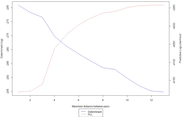
The estimation of Model D is straightforward. It simply consists in re-estimating Model C while accounting for the panel nature of the data by adding a random effect parameter, σ. The model is estimated using MSL and 1,000 Halton draws. On the other hand and as previously introduced in Section 3.5, finding the best autoregressive model using CML requires to estimate a series of models with an increasing number of related pairs of observations for the same individual. We start by estimating a model where each bivariate pair is not separated by more than two years and increase this number until the logarithm of the determinant of the robust variance-covariance matrix for each estimated model stops increasing (or decreases). Results are reported in Table3 and Figure2.
Figure 2: Trace and Predictive Log-Likelihood
In addition of the logarithm of the determinant, we also compute the predictive log- likelihood for each model (Castro et al.,2013), which allows to compare the goodness-of- fit of the CML models to Model A, B, C and D. The results indicate that the adequate distance between pairs is 14 years. Interestingly, the model which features the best value for the logarithm of the determinant is also the model which features the best predictive log-likelihood. Having established the right model composition for Model E, we move on to comparing Model D and Model E.
Table 3: Goodness-of-fit indicators d Determinant PLL 2 -264.0736 -4182.26 3 -266.6883 -4179.959 4 -268.4825 -4160.955 5 -275.2321 -4062.872 6 -278.8054 -4022.956 7 -281.5748 -3997.095
8 -284.112 -3978.297
9 -286.5214 -3964.236 10 -287.1156 -3959.526 11 -290.237 -3949.051 12 -292.9751 -3944.075 13 -294.8523 -3942.283 14 -295.1941 -3942.258
The results for Model D and E are reported in Table 4 below. The main result is that the autoregressive specification, Model E, largely outperforms the static one, Model D, in terms of predicting log-likelihood (-6320.049 versus -3942.258). In addition, ρ, the parameter which regulates the AR1 process in Model E, is found to be strongly significant. These results clearly indicate that modelling car availability as a dynamic process improves model performances. In addition, Model E features smaller standard errors for most parameters in comparison to Model D, which is likely to be induced by the fact that some of the noise in the data is now captured by the autocorrelation parameter, ρ. These quantitative results confirm the qualitative insights ofClark et al.
(2016). We now move on to the interpretation of the model parameters, which requires the computation of marginal effects.
5.3 Model interpretation and marginal effects
Parameters interpretation in probit regression is not straightforward. A detailed analysis of the results is further complicated by the generalized structure used in this paper.
As previously mentioned, a positive parameter in the latent car availability propensity equation means that an increase in the given independent variable leads to an increase in observing a higher outcome. However, a positive parameter in the Interactions with threshold 2 equation means that an increase in the given independent variable leads to a decrease in observing a higher car availability outcome. To facilitate the interpretation of the results from the Random effects generalized ordered probit model and the AR1 Random effects generalized ordered probit, we compute the marginal effects1 for the most
1Also known as partial effects in the literature.
Table 4: Model results
Model D Model E
Log-Likelihood -6320.049 Predictive log-likelihood -3942.258
AIC 12774.1
CM (Log)-Likelihood -511.5514
BIC 13303.78
Parameters
Latent car availability propensity
Thresholds and interac-
tions with threshold 2 Parameters
Latent car availability propensity
Thresholds and interac- tions with threshold 2 Coefficient Robust T. Coefficient Robust T. Coefficient Robust T. Coefficient Robust T.
Threshold1 . . 4.0868 5.2 Threshold1 . . 2.3502 3.47
Threshold2 . . -1.1411 -1.6 Threshold2 . . -1.1609 -2.05
female -1.754 -4.94 0.151 1.14 female -1.3117 -5.29 0.077 0.57
age 0.0309 2.01 0.0028 0.31 age 0.0244 2.52 -0.0044 -0.61
distw 0.0059 0.89 -0.0044 -0.63 distw 0.0194 1.95 0.0059 0.91
german 1.032 1.94 0.454 1.34 german 0.3021 0.65 0.158 0.5
own home 0.3183 1.43 0.2536 1.82 own home 0.5352 2.98 0.3407 2.37
moped -0.8425 -2.29 -0.6148 -1.2 moped -0.3915 -1.18 -0.5741 -1.23
moving -0.0535 -0.76 -0.0397 -0.89 moving -0.08 -1.59 -0.0702 -1.62
children 0.0722 0.62 0.0296 0.46 children 0.0194 0.23 0.077 1.26
birth 0.0946 1.03 0.0667 1.37 birth 0.0308 0.49 -0.0284 -0.63
married 0.6628 3.73 0.4809 3.49 married 0.4006 2.95 0.3551 2.34
wed -0.1793 -1.43 -0.1325 -1.42 wed -0.0733 -0.74 -0.0848 -0.96
license moped 1.2269 2.11 0.0523 0.35 license moped 0.1746 0.75 0.0647 0.47
license car 3.8801 7.8 0.4813 1.09 license car 2.9127 7.19 0.6356 2.18
central2 -0.1769 -0.61 -0.0034 -0.02 central2 0.2009 0.97 0.1167 0.66
central3 -0.3637 -1.29 -0.3096 -1.2 central3 0.1561 0.85 -0.1976 -0.98
central4 0.0038 0.01 0.0597 0.29 central4 0.2786 1.25 0.2313 1.21
central5 0.3284 1.1 0.0837 0.38 central5 0.3571 1.75 0.0948 0.53
pop1 0.2404 0.4 -0.5873 -1.05 pop1 -1.0571 -1.87 -1.1706 -1.67
pop2 -0.3853 -0.87 -0.6293 -1.81 pop2 -0.4023 -1.22 -0.6954 -2.17
pop3 -0.1441 -0.43 -0.248 -1.28 pop3 -0.2372 -0.78 -0.2266 -1.07
pop5 0.2274 0.65 -0.0463 -0.29 pop5 -0.0165 -0.04 0.0075 0.03
pop6 0.0806 0.26 -0.1508 -0.93 pop6 -0.1118 -0.4 -0.0729 -0.42
pop7 0.1921 0.64 -0.1087 -0.61 pop7 -0.2975 -1.01 -0.1589 -0.78
edu training 1.1061 2.14 -0.1398 -0.8 edu training 0.5777 1.89 -0.0734 -0.4
edu uni 0.6613 1.32 -0.3864 -1.91 edu uni 0.3598 1.15 -0.3619 -1.7
edu other 1.5324 2.51 0.0471 0.24 edu other 0.9639 2.62 0.0938 0.45
degree 0.8534 4.13 0.4242 2.4 degree 0.4481 2.64 0.3975 2.06
home det house 0.2219 1.04 -0.0324 -0.22 home det house 0.018 0.09 -0.1426 -0.87
home semi det house 0.0244 0.09 -0.1679 -0.87 home semi det house -0.2807 -1.34 -0.3105 -1.56
home townhouse 0.1154 0.36 -0.0648 -0.36 home townhouse -0.1619 -0.69 -0.0856 -0.48
home aprt big 0.116 0.29 0.189 0.56 home aprt big 0.0011 0 0.1465 0.66
home other -0.5194 -2.15 -0.6047 -2.23 home other -0.3868 -1.75 -0.7562 -2.78
σ(rand. effect) 2.9987 14.7 . . σ(rand. effect) 1.623 7.04 . .
ρ . . . . Rho 2.6441 11.54 . .
significant parameters. Marginal effects can simply be described as the effect of a discrete variation of a given predictorxon the probability of observing the modelled outcome all else being equal.
5.3.1 Computation
Details on the computation of marginal effects in the context of probit models are given by Greene and Hensher (2010). Following the notations established in Equation 4 and accounting for the fact that most of the variables used in this analysis appear in both Y∗ andµ2, it comes that
δP rob(Y =k|x, z)
δx = (φ(µk−β0x)−φ(µk−1−β0x))β (13)
and
δP rob(Y =k|x, z)
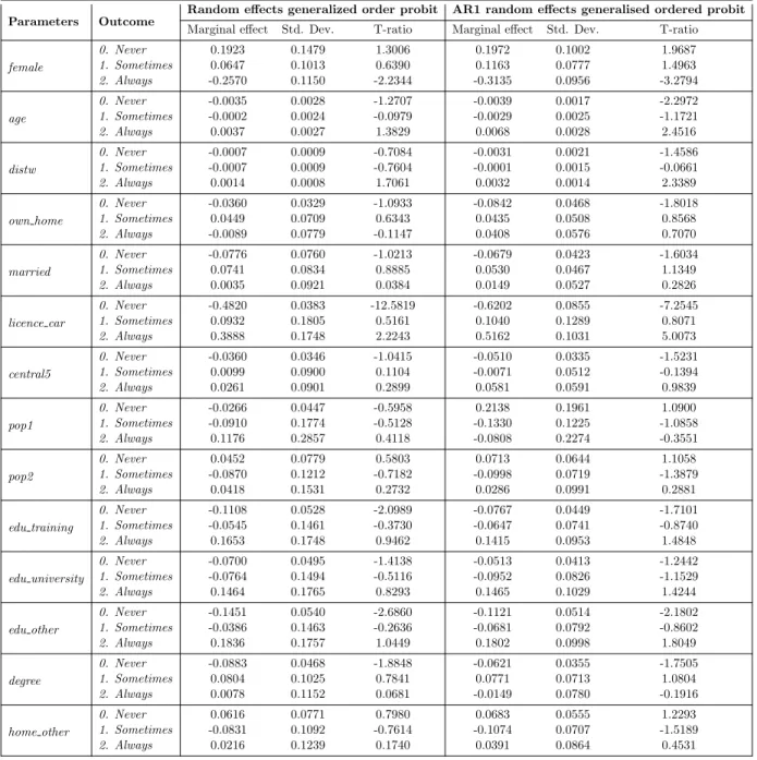
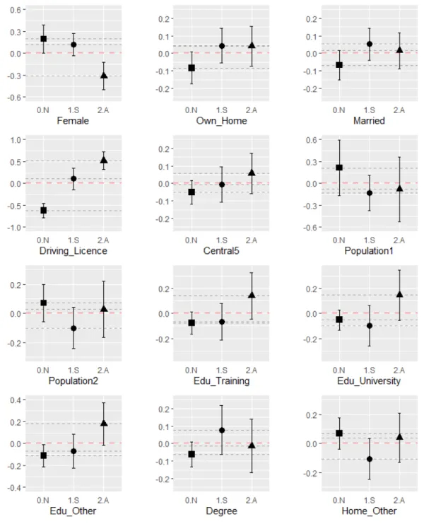
δz = (φ(µk−β0x)µkζk−φ(µk−1−β0x))µk−1ζk−1 (14) We compute the marginal effects for the three outcome considered ([Car] ”0. Never available”, ”1. Sometimes available” and ”2. Always available”) and the models with and without autocorrelation. This allows us to give richer comments on the differences in terms of behavioural interpretations provided by the two models as well as to further demonstrate the need to account for autocorrelation in large panel datasets such as those typically found in life-course analysis. Results are reported in Table5below. Given that the marginal effects are computed ”at means”, that is by assuming during computations that the values for all the predictors is at their corresponding mean, some marginal effects are not found to be significant although their corresponding parameters in Table4 are.
In this paper, we only compute the marginal effects for the parameters which have been found to be significant in the model estimation phase.
5.3.2 Interpretation
We describe how to interpret the results from Table 5 by taking the example of the variablefemale for Model E. According to the model results, being a woman with respect to being a man increases the probability of reporting a car as never available by 0.1972 while it decreases the probability of reporting a car as Always available by 0.3135. For continuous variables (ageanddistw (distance to work)), the values correspond to a shift in outcome probability for a unit increase.
We report differences between Model D and Model E. In particular, we find that the marginal effects derived from both models are similar in sign, but that the simple random effects models fails to capture effects which are typically considered to be strongly significant in the literature in some cases. For example, the variable f emale, for which