Spectra of ‘‘real-world’’ graphs: Beyond the semicircle law
Ille´s J. Farkas,1,*Imre Dere´nyi,2,3,†Albert-La´szlo´ Baraba´si,2,4,‡and Tama´s Vicsek1,2,§
1Department of Biological Physics, Eo¨tvo¨s University, Pa´zma´ny Pe´ter Se´ta´ny 1A, H-1117 Budapest, Hungary
2Collegium Budapest, Institute for Advanced Study, Szentha´romsa´g utca 2, H-1014 Budapest, Hungary
3Institut Curie, UMR 168, 26 rue d’Ulm, F-75248 Paris 05, France
4Department of Physics, University of Notre Dame, Notre Dame, Indiana 46556 共Received 19 February 2001; published 20 July 2001兲
Many natural and social systems develop complex networks that are usually modeled as random graphs. The eigenvalue spectrum of these graphs provides information about their structural properties. While the semi- circle law is known to describe the spectral densities of uncorrelated random graphs, much less is known about the spectra of real-world graphs, describing such complex systems as the Internet, metabolic pathways, net- works of power stations, scientific collaborations, or movie actors, which are inherently correlated and usually very sparse. An important limitation in addressing the spectra of these systems is that the numerical determi- nation of the spectra for systems with more than a few thousand nodes is prohibitively time and memory consuming. Making use of recent advances in algorithms for spectral characterization, here we develop meth- ods to determine the eigenvalues of networks comparable in size to real systems, obtaining several surprising results on the spectra of adjacency matrices corresponding to models of real-world graphs. We find that when the number of links grows as the number of nodes, the spectral density of uncorrelated random matrices does not converge to the semicircle law. Furthermore, the spectra of real-world graphs have specific features, depending on the details of the corresponding models. In particular, scale-free graphs develop a trianglelike spectral density with a power-law tail, while small-world graphs have a complex spectral density consisting of several sharp peaks. These and further results indicate that the spectra of correlated graphs represent a practical tool for graph classification and can provide useful insight into the relevant structural properties of real networks.
DOI: 10.1103/PhysRevE.64.026704 PACS number共s兲: 02.60.⫺x, 68.55.⫺a, 68.65.⫺k, 05.45.⫺a
I. INTRODUCTION
Random graphs 关1,2兴 have long been used for modeling the evolution and topology of systems made up of large as- semblies of similar units. The uncorrelated random graph model—which assumes each pair of the graph’s vertices to be connected with equal and independent probabilities—
treats a network as an assembly of equivalent units. This model, introduced by the mathematicians Paul Erdo˝s and Al- fre´d Re´nyi关1兴, has been much investigated in the mathemati- cal literature 关2兴. However, the increasing availability of large maps of real-life networks has indicated that real net- works are fundamentally correlated systems, and in many respects their topology deviates from the uncorrelated ran- dom graph model. Consequently, the attention has shifted towards more advanced graph models which are designed to generate topologies in line with the existing empirical results 关3–14兴. Examples of real networks, that serve as a bench- mark for the current modeling efforts, include the Internet 关6,15–17兴, the World-Wide Web关8,18兴, networks of collabo- rating movie actors and those of collaborating scientists 关13,14兴, the power grid关4,5兴, and the metabolic network of numerous living organisms 关9,19兴.
These are the systems that we will call ‘‘real-world’’ net- works or graphs. Several converging reasons explain the en- hanced current interest in such real graphs. First, the amount of topological data available on such large structures has increased dramatically during the past few years thanks to the computerization of data collection in various fields, from sociology to biology. Second, the hitherto unseen speed of growth of some of these complex networks—e.g., the Internet—and their pervasiveness in affecting many aspects of our lives has created the need to understand the topology, origin, and evolution of such structures. Finally, the in- creased computational power available on almost every desktop has allowed us to study such systems in unpre- cedented detail.
The proliferation of data has lead to a flurry of activity towards understanding the general properties of real net- works. These efforts have resulted in the introduction of two classes of models, commonly called small-world graphs 关4,5兴 and the scale-free networks 关10,11兴. The first aims to capture the clustering observed in real graphs, while the sec- ond reproduces the power-law degree distribution present in many real networks. However, until now, most analyses of these models and data sets have been confined to real-space characteristics, which capture their static structural properties e.g., degree sequences, shortest connecting paths, and clus- tering coefficients. In contrast, there is extensive literature demonstrating that the properties of graphs and the associ- ated adjacency matrices are well characterized by spectral methods, that provide global measures of the network prop- erties关20,21兴. In this paper we offer a detailed analysis of the
*Email address: fij@elte.hu
†Email address: derenyi@angel.elte.hu
‡Email address: alb@nd.edu
§Email address: vicsek@angel.elte.hu
most studied network models using algebraic tools intrinsic to large random graphs.
The paper is organized as follows. Section II introduces the main random graph models used for the topological de- scription of large assemblies of connected units. Section III lists the—analytical and numerical—tools that we used and developed to convert the topological features of graphs into algebraic invariants. Section IV contains our results concern- ing the spectra and special eigenvalues of the three main types of random graph models: sparse uncorrelated random graphs in Sec. IV A, small-world graphs in Sec. IV B, and scale-free networks in Sec. IV C. Section IV D gives simple algorithms for testing the graph’s structure, and Sec. IV E investigates the variance of structure within single random graph models.
II. MODELS OF RANDOM GRAPHS A. The uncorrelated random graph model
and the semicircle law 1. Definitions
Throughout this paper we will use the term ‘‘graph’’ for a set of points共vertices兲connected by undirected lines共edges兲; no multiple edges and no loops connecting a vertex to itself are allowed. We will call two vertices of the graph ‘‘neigh- bors,’’ if they are connected by an edge. Based on Ref.关1兴, we shall use the term ‘‘uncorrelated random graph’’ for a graph if共i兲the probability for any pair of the graph’s vertices being connected is the same, p; 共ii兲 these probabilities are independent variables.
Any graph G can be represented by its adjacency matrix A(G), which is a real symmetric matrix: Ai j⫽Aji⫽1, if vertices i and j are connected, or 0, if these two vertices are not connected. The main algebraic tool that we will use for the analysis of graphs will be the spectrum—i.e., the set of eigenvalues—of the graph’s adjacency matrix. The spectrum of the graph’s adjacency matrix is also called the spectrum of the graph.
2. Applying the semicircle law for the spectrum of the uncorrelated random graph
A general form of the semicircle law for real symmetric matrices is the following关20,22,23兴. If A is a real symmetric N⫻N uncorrelated random matrix, 具Ai j典⬅0 and具Ai j
2典⫽2 for every i⫽j , and with increasing N each moment of each 兩Ai j兩 remains finite, then in the N→⬁ limit the spectral density—i.e., the density of eigenvalues—of A/
冑
N con-verges to the semicircular distribution
共兲⫽
再
共02otherwise.2兲⫺1冑
42⫺2 if 兩兩⬍2 共1兲This theorem is also known as Wigner’s law关22兴, and its extensions to further matrix ensembles have long been used for the stochastic treatment of complex quantum-mechanical systems lying far beyond the reach of exact methods关24,25兴.
Later, the semicircle law was found to have many applica- tions in statistical physics and solid-state physics as well 关20,21,26兴.
Note, that for the adjacency matrix of the uncorrelated random graph many of the semicircle law’s conditions do not hold, e.g., the expectation value of the entries is a nonzero constant: p⫽0. Nevertheless, in the N→⬁ limit, the re- scaled spectral density of the uncorrelated random graph converges to the semicircle law of Eq.共1兲 关27兴. An illustra- tion of the convergence of the average spectral density to the semicircular distribution can be seen on Fig. 1. It is neces- sary to make a comment concerning figures here. In order to keep figures simple, for the spectral density plots we have chosen to show the spectral density of the original matrix A and to rescale the horizontal 共兲 and vertical 共兲 axes by
⫺1N⫺1/2⫽关N p(1⫺p)兴⫺1/2andN1/2⫽关N p(1⫺p)兴1/2. Some further results on the behavior of the uncorrelated random graph’s eigenvalues, relevant for the analysis of real- world graphs as well, include the following: The principal eigenvalue 共the largest eigenvalue 1) grows much faster than the second eigenvalue: limN→⬁(1/N)⫽p with prob- ability 1, whereas for every⑀⬎1/2, limN→⬁(2/N⑀)⫽0 共see Refs. 关27,28兴 and Fig. 1兲. A similar relation holds for the smallest eigenvalue N: for every ⑀⬎1/2, limN→⬁(N/N⑀)
⫽0. In other words, if具ki典 denotes the average number of connections of a vertex in the graph, then 1 scales as pN
⬇具ki典, and the width of the ‘‘bulk’’ part of the spectrum, the set of the eigenvalues兵2, . . . ,N其, scales as
冑
N. Lastly,the semicircular distribution’s edges are known to decay FIG. 1. If N→⬁and p⫽const, the average spectral density of an uncorrelated random graph converges to a semicircle, the first eigenvalue grows as N, and the second is proportional to冑N 共see Sec. II A兲. Main panel: The spectral density is shown for p⫽0.05 and three different system sizes: N⫽100共—兲, N⫽300共– –兲, and N⫽1000共- - -兲. In all three cases, the complete spectrum of 1000 graphs was computed and averaged. Inset: At the edge of the semi- circle, i.e., in the ⬇⫾2冑N p(1⫺p) regions, the spectral density decays exponentially, and with N→⬁, the decay rate diverges 关20,29兴. Here, F()⫽N⫺1兺i⬍1 is the cumulative spectral distri- bution function, and 1⫺F is shown for a graph with N⫽3000 vertices and 15 000 edges.
exponentially, and the number of eigenvalues in the
⬎O(
冑
N) tail has been shown to be of the order of 1关20,29兴.B. Real-world graphs
The two main models proposed to describe real-world graphs are the small-world model and the scale-free model.
1. Small-world graphs
The small-world graph 关4,5,30兴 is created by randomly rewiring some of the edges of a regular关31兴ring graph. The regular ring graph is created as follows. First draw the ver- tices 1,2, . . . ,N on a circle in ascending order. Then, for every i, connect vertex i to the vertices lying closest to it on the circle: vertices i⫺k/2, . . . ,i⫺1,i⫹1, . . . ,i⫹k/2, where every number should be understood modulo N (k is an even number兲. Figure 9 will show later that this algorithm creates a regular graph indeed, because the degree关31兴of any vertex is the same number k. Next, starting from vertex 1 and pro- ceeding towards N, perform the rewiring step. For vertex 1, consider the first ‘‘forward connection,’’ i.e., the connection to vertex 2. With probability pr, reconnect vertex 1 to an- other vertex chosen uniformly at random and without allow- ing multiple edges. Proceed toward the remaining forward connections of vertex 1, and then perform this step for the remaining N⫺1 vertices also. For the rewiring, use equal and independent probabilities. Note that in the small-world model the density of edges is p⫽具ki典/(N⫺1)⬇k/N.
Throughout this paper, we will use only k⬎2.
If we use pr⫽0 in the small-world model, the original regular graph is preserved, and for pr⫽1, one obtains a ran- dom graph that differs from the uncorrelated random graph only slightly: every vertex has a minimum degree of k/2.
Next, we will need two definitions. The separation between vertices i and j, denoted by Li j, is the number of edges in the shortest path connecting them. The clustering coefficient at vertex i, denoted by Ci, is the number of existing edges among the neighbors of vertex i divided by the number of all possible connections between them. In the small-world model, both Li j and Ci are functions of the rewiring prob- ability pr. Based on the above definitions of Li j( pr) and Ci( pr), the characteristics of the small-world phenomenon, which occurs for intermediate values of pr, can be given as follows 关4,5兴:共i兲the average separation between two verti- ces, L( pr), drops dramatically below L( pr⫽0), whereas共ii兲 the average clustering coefficient C( pr) remains high, close to C( pr⫽0). Note that the rewiring procedure is carried out independently for every edge; therefore, the degree sequence and also other distributions in the system, e.g., path length and loop size, decay exponentially.
2. The scale-free model
The scale-free model assumes a random graph to be a growing set of vertices and edges, where the location of new edges is determined by a preferential attachment rule 关10,11兴. Starting from an initial set of m0 isolated vertices, one adds one new vertex and m new edges at every time step t. 共Throughout this paper, we will use m⫽m0.兲The m new
edges connect the new vertex and m different vertices chosen from the N old vertices. The ith old vertex is chosen with probability ki/兺j⫽1,Nkj, where ki is the degree of vertex i.
关The density of edges in a scale-free graph is p⫽具ki典/(N
⫺1)⬇2m/N.兴In contrast to the small-world model, the dis- tribution of degrees in a scale-free graph converges to a power law when N→⬁, which has been shown to be a com- bined effect of growth and the preferential attachment 关11兴. Thus, in the infinite time or size limit, the scale-free model has no characteristic scale in the degree size关14,32–37兴.
3. Related models
Lately, numerous other models have been suggested for a unified description of real-world graphs 关14,32–35,37–40兴. Models of growing networks with aging vertices were found to display both heavy tailed and exponentially decaying de- gree sequences 关34–36兴as a function of the speed of aging.
Generalized preferential attachment rules have helped us bet- ter understand the origin of the exponents and correlations emerging in these systems 关32,33兴. Also, investigations of more complex network models—using aging or an additional fixed cost of edges 关12兴 or preferential growth and random rewiring 关37兴—have shown, that in the ‘‘frequent rewiring, fast aging, high cost’’ limiting case, one obtains a graph with an exponentially decaying degree sequence, whereas in the
‘‘no rewiring, no aging, zero cost’’ limiting case the degree sequence will decay as a power law. According to studies of scientific collaboration networks 关13,14兴 and further social and biological structures关12,19,41兴, a significant proportion of large networks lies between the two extremes. In such cases, the characterization of the system using a small num- ber of algebraic constants could facilitate the classification of real-world networks.
III. TOOLS A. Analytical 1. The spectrum of the graph
The spectrum of a graph is the set of eigenvalues of the graph’s adjacency matrix. The physical meaning of a graph’s eigenpair 共an eigenvector and its eigenvalue兲 can be illus- trated by the following example. Write each component of a vector vជ on the corresponding vertex of the graph: vi on vertex i. Next, on every vertex write the sum of the numbers found on the neighbors of vertex i. If the resulting vector is a multiple ofvជ, thenvជ is an eigenvector, and the multiplier is the corresponding eigenvalue of the graph.
The spectral density of a graph is the density of the eigen- values of its adjacency matrix. For a finite system, this can be written as a sum of␦ functions
共兲ª1
N
兺
j⫽N1 ␦共⫺j兲, 共2兲which converges to a continuous function with N→⬁ (j is the jth largest eigenvalue of the graph’s adjacency matrix兲.
The spectral density of a graph can be directly related to the graph’s topological features: the kth moment Mkof共兲 can be written as
Mk⫽1
N j
兺
⫽N1 共j兲k⫽N1Tr共Ak兲⫽1 N i
兺
1,i2,•••,ik
Ai
1,i2Ai
2,i3•••Ai
k,i1. 共3兲
From the topological point of view, Dk⫽N Mkis the num- ber of directed paths 共loops兲 of the underlying—
undirected—graph, that return to their starting vertex after k steps. On a tree, the length of any such path can be an even number only, because these paths contain any edge an even number of times: once such a path has left its starting point by choosing a starting edge, no alternative route for returning to the starting point is available. However, if the graph con- tains loops of odd length, the path length can be an odd number, as well.
2. Extremal eigenvalues
In an uncorrelated random graph the principal eigenvalue
1 shows the density of edges and 2 can be related to the conductance of the graph as a network of resistances 关42兴. An important property of all graphs is the following: the principal eigenvector eជ1 of the adjacency matrix is a non- negative vector共all components are non-negative兲, and if the graph has no isolated vertices, eជ1 is a positive vector 关43兴. All other eigenvectors are orthogonal to eជ1, therefore they all have entries with mixed signs.
3. The inverse participation ratios of eigenvectors The inverse participation ratio of the normalized j th ei- genvector eជj is defined as关26兴
Ij⫽k
兺
⫽N1 关共ej兲k兴4. 共4兲If the components of an eigenvector are identical, (ej)i
⫽1/
冑
N for every i, then Ij⫽1/N. For an eigenvector with one single nonzero component, (ej)i⫽␦i,i⬘, the inverse par- ticipation ratio is 1. The comparison of these two extremal cases illustrates that with the help of the inverse participation ratio, one can tell whether only O(1) or as many as O(N) components of an eigenvector differ significantly from 0, i.e., whether an eigenvector is localized or nonlocalized.B. Numerical
1. General real symmetric eigenvalue solver
To compute the eigenpairs of graphs below the size N
⫽5000, we used the general real symmetric eigenvalue solver of Ref.关44兴. This algorithm requires the allocation of memory space to all entries of the matrix, thus to compute the spectrum of a graph of size N⫽20 000 (N⫽1 000 000) using this general method with double precision floating point arithmetic, one would need 3.2 GB 共8 TB兲 memory
space and the execution of approximately 30N2⫽1.2⫻1010 (3⫻1013) floating point operations 关44兴. Consequently, we need to develop more efficient algorithms to investigate the properties of graphs with sizes comparable to real-world net- works.
2. Iterative eigenvalue solver based on the thick-restart Lanczos algorithm
The spectrum of a real-world graph is the spectrum of a sparse real symmetric matrix; therefore, the most efficient algorithms that can give a handful of the top nd eigenvalues—and the corresponding eigenvectors—of a large graph are iterative methods关45兴. These methods allow the matrix to be stored in any compact format, as long as matrix-vector multiplication can be carried out at a high speed. Iterative methods use little memory: only the nonzero entries of the matrix and a few vectors of size N need to be stored. The price for computational speed lies in the number of the obtained eigenvalues: iterative methods compute only a handful of the largest共or smallest兲eigenvalues of a matrix.
To compute the eigenvalues of graphs above the size N
⫽5 000, we have developed algorithms using a specially modified version of the thick-restart Lanczos algorithm 关46,47兴. The modifications and some of the main technical parameters of our software are explained in the following paragraphs.
Even though iterative eigenvalue methods are mostly used to obtain the top eigenvalues of a matrix, after minor modi- fications the internal eigenvalues in the vicinity of a fixed
⫽0 point can be computed as well. For this, extremely sparse matrices are usually ‘‘shift-inverted,’’ i.e., to find those eigenvalues of A that are closest to0, the highest and lowest eigenvalues of (A⫺0I)⫺1 are searched for. How- ever, because of the extremely high cost of matrix inversion in our case, for the computation of internal eigenvalues we suggest using the ‘‘shift-square’’ method with the matrix
B⫽关*/2⫺共A⫺0I兲2兴2n⫹1. 共5兲
Here*is the largest eigenvalue of (A⫺0I)2, I is the iden- tity matrix, and n is a positive integer. Transforming the matrix A into B transforms the spectrum of A in the follow- ing manner. First, the spectrum is shifted to the left by 0. Then, the spectrum is ‘‘folded’’ 共and squared兲 at the origin such that all eigenvalues will be negative. Next, the spectrum is linearly rescaled and shifted to the right, with the follow- ing effect: 共i兲 the whole spectrum will lie in the symmetric interval 关⫺*/2,*/2兴 and 共ii兲 those eigenvalues that were closest to 0 in the spectrum of A will be the largest now, i.e., they will be the eigenvalues closest to */2. Now, rais- ing all eigenvalues to the (2n⫹1)st power increases the relative difference, 1⫺i/j, between the top eigenvalues
i and j by a factor of 2n⫹1. This allows the iterative method to find the top eigenvalues of B more quickly. One can compute the corresponding eigenvalues 共those being closest to0) of the original matrix, A: if bជ1,bជ2, . . . ,bជn
dare the normalized eigenvectors of the ndlargest eigenvalues of
B, then for A the nd eigenvalues closest to 0 will be, not necessarily in ascending order, bជ1Abជ1,bជ2Abជ2, . . . ,bជn
dAbជn
d. The thick-restart Lanczos method uses memory space for the nonzero entries of the N⫻N large adjacency matrix, and ng⫹1 vectors of length N, where ng(ng⬎nd) is usually be- tween 10 and 100. Besides the relatively small size of re- quired memory, we could also exploit the fact that the non- zero entries of a graph’s adjacency matrix are all 1’s: during matrix-vector multiplication—which is usually the most time-consuming step of an iterative method—only additions had to be carried out instead of multiplications.
The numerical spectral density functions of large graphs (N⭓5000) of this paper were obtained using the following steps. To compute the spectral density of the adjacency ma- trix A at an internal⫽0 location, first the ndeigenvalues closest to0 were searched for. Next, the distance between the smallest and the largest of the obtained eigenvalues was computed. Finally, to obtain (0) this distance was multi- plied by N/(nd⫺1), and was averaged using nav different graphs. We used double precision floating point arithmetic, and the iterations were stopped if共i兲at least nititerations had been carried out and 共ii兲the lengths of the residual vectors belonging to the nd selected eigenpairs were all below
⫽10⫺12关46兴.
IV. RESULTS
A. Sparse uncorrelated random graphs:
The semicircle law is not universal
In the uncorrelated random graph model of Erdo˝s and Re´nyi, the total number of edges grows quadratically with the number of vertices: Nedge⫽N具ki典⫽N p(N⫺1)⬇pN2. However, in many real-world graphs edges are ‘‘expensive,’’
and the growth rate of the number of connections remains well below this rate. For this reason, we also investigated the spectra of such uncorrelated networks, for which the prob- ability of any two vertices being connected changes with the size of the system using pN␣⫽c⫽const. Two special cases are ␣⫽0 共the Erdo˝s-Re´nyi model兲 and ␣⫽1. In the second case, pN→const as N→⬁, i.e., the average degree remains constant.
For ␣⬍1 and N→⬁, there exists an infinite cluster of connected vertices 共in fact, it exists for every ␣⭐1 关2兴兲. Moreover, the expectation value of any ki converges to in- finity, thus any vertex is almost surely connected to the infi- nite cluster. The spectral density function converges to the semicircular distribution of Eq.共1兲because the total weight of isolated subgraphs decreases exponentially with growing system size. 共A detailed analysis of this issue is available in Ref. 关48兴.兲
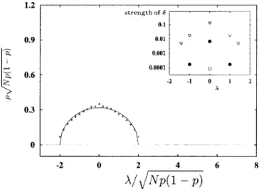
For ␣⫽1 and N→⬁ 共see Fig. 2兲, the probability for a vertex to belong to a cluster of any finite size remains also finite 关49兴. Therefore, the limiting spectral density contains the weighted sum of the spectral densities of all finite graphs 关50兴. The most striking deviation from the semicircle law in this case is the elevated central part of the spectral density.
The probability for a vertex to belong to an isolated cluster of size s decreases exponentially with s 关49兴; therefore, the
number of large isolated clusters is low. The eigenvalues of a graph with s vertices are bounded by ⫺
冑
s⫺1 and冑
s⫺1.For these two reasons, the amplitudes of ␦ functions decay exponentially, as the absolute value of their locations, 兩兩, increases.
The principal eigenvalue of this graph converges to a con- stant: limN→⬁(1)⫽pN⫽c, and 共兲 will be symmetric in the N→⬁ limit. Therefore, in the limit, all odd moments ( M2k⫹1), and thus the number of all loops with odd length (D2k⫹1), disappear. This is a salient feature of graphs with tree structure共because on a tree every edge must be used an even number of times in order to return to the initial vertex兲, indicating that the structure of a sparse uncorrelated random graph becomes more and more treelike. This can also be understood by considering that the typical distance共length of the shortest path兲between two vertices on both a sparse un- correlated random graph and a regular tree with the same number of edges scales as ln(N). So except for a few short- cuts a sparse uncorrelated random graph looks like a tree.
B. The small-world graph Triangles are abundant in the graph
For pr⫽0 the small-world graph is regular and also pe- riodical. Because of the highly ordered structure, 共兲 con- tains numerous singularities, which are listed in Sec. VI A 共see also Fig. 3兲. Note that共兲 has a high third moment.
共Remember, that we use only k⬎2.兲
FIG. 2. If N→⬁ and pN⫽const, the spectral density of the uncorrelated random graph does not converge to a semicircle. Main panel: Symbols show the spectrum of an uncorrelated random graph共20 000 vertices and 100 000 edges兲measured with the itera- tive method using nav⫽1, nd⫽101, and ng⫽250. A solid line shows the semicircular distribution for comparison.共Note that the principal eigenvalue 1 is not shown here because here at any0
point the average first-neighbor distance among nd⫽101 eigenval- ues was used to measure the spectral density.兲Inset: Strength of␦ functions in共兲‘‘caused’’ by isolated clusters of sizes 1, 2, and 3 in uncorrelated random graphs 共see Ref.关50兴for a detailed expla- nation兲. Symbols are for graphs with 20 000 vertices and 20 000 edges共ⵜ兲, 50 000 edges共䊉兲, and 100 000 edges共䊊兲. Results were averaged for three different graphs everywhere.
If we increase pr such that the small-world region is reached, i.e., the periodical structure of the graph is per- turbed, then singularities become blurred and are trans- formed into high local maxima, but 共兲 retains a strong skewness 共see Fig. 3兲. This is in good agreement with the results of Refs. 关30,51兴, where it has been shown that the local structure of the small-world graph is ordered; however, already a very small number of shortcuts can drastically change the graph’s global structure.
In the pr⫽1 case the small-world model becomes very similar to the uncorrelated random graph: the only difference is that here, the minimum degree of any vertex is a positive constant k/2, whereas in an uncorrelated random graph the degree of a vertex can be any non-negative number. Accord- ingly,共兲 becomes a semicircle for pr⫽1 共Fig. 3兲. Never- theless, it should be noted that as pr converges to 1, a high value of M3 is preserved even for pr close to 1, where all local maxima have already vanished. The third moment of
共兲 gives the number of triangles in the graph 共see Sec.
III A 1兲; the lack of high local maxima, i.e., the remnants of singularities, shows the absence of an ordered structure.
From the above we conclude, that—from the spectrum’s point of view—the high number of triangles is one of the most basic properties of the small-world model, and it is preserved much longer than regularity or periodicity if the
level of randomness pr is increased. This is in good agree- ment with the results of Ref.关19兴where the high number of small cycles is found to be a fundamental property of small- world networks. As an application, the high number of small cycles results in special diffusion on small-world graphs 关61兴.
C. The scale-free graph
For m⫽m0⫽1, the scale-free graph is a tree by definition and its spectrum is symmetric 关43兴. In the m⬎1 case 共兲 consists of several well distinguishable parts 共see Fig. 4兲. The ‘‘bulk’’ part of the spectral density—the set of the eigen- values 兵2, . . . ,N其—converges to a symmetric continuous function which has a trianglelike shape for the normalized values up to 1.5 and has power-law tails.
The central part of the spectral density lies well above the semicircle. Since the scale-free graph is fully connected by definition, the increased number of eigenvalues with small magnitudes cannot be accounted to isolated clusters, as be- fore in the case of the sparse uncorrelated random graph. As an explanation, we suggest, that the eigenvectors of these eigenvalues are localized on a small subset of the graph’s vertices. 共This idea is supported by the high inverse partici- pation ratios of these eigenvectors, see Fig. 7.兲
1. The spectral density of the scale-free graph decays as a power law
The inset of Fig. 4 shows the tail of the bulk part of the spectral density for a graph with N⫽40 000 vertices and FIG. 3. Spectral densities of small-world graphs using the com-
plete spectra. The solid line shows the semicircular distribution for comparison. 共a兲 Spectral density of the regular ring graph created from the small-world model with pr⫽0, k⫽10, and N⫽1000. 共b兲 For pr⫽0.01, the average spectral density of small-world graphs contains sharp maxima, which are the ‘‘blurred’’ remnants of the singularities of the pr⫽0 case. Topologically, this means that the graph is still almost regular, but it contains a small number of im- purities. In other words, after a small perturbation, the system is no longer degenerate. 共c兲 The average spectral density computed for the pr⫽0.3 case shows that the third moment of共兲is preserved even for very high values of pr, where there is already no sign of any blurred singularity共i.e., regular structure兲. This means that even though all remaining regular islands have been destroyed already, triangles are still dominant.共d兲 If pr⫽1, then the spectral density of the small-world graph converges to a semicircle. In共b兲,共c兲, and 共d兲, 1000 different graphs with N⫽1000 and k⫽10 were used for averaging.
FIG. 4. Main panel: The average spectral densities of scale-free graphs with m⫽m0⫽5 and N⫽100共—兲, N⫽1000共– –兲, and N
⫽7000共- - -兲vertices.共In all three cases, the complete spectrum of 1000 graphs was used.兲Another continuous line shows the semicir- cular distribution for comparison. Observe that共i兲the central part of the scale-free graph’s spectral density is trianglelike, not semicircu- lar and共ii兲 the edges show a power-law decay, whereas the semi- circular distribution’s edges decay exponentially, i.e., it decays ex- ponentially at the edges关20兴. Inset: The upper edge of the spectral density for scale-free graphs with N⫽40 000 vertices, the average degree of a vertex being 具ki典⫽2m⫽10 as before. Note that both axes are logarithmic, indicating that共兲has a power-law tail. Here we used the iterative eigenvalue solver of Sec. III B 2 with nd
⫽21, nav⫽3, and ng⫽60. The line with the slope⫺5 in this figure is a guide to the eye.
200 000 edges共i.e., pN⫽10). Comparing this to the inset of Fig. 1, where the number of vertices and edges is the same as here, one can observe the power-law decay at the edge of the bulk part of 共兲. As shown later, in Sec. IV D, the power- law decay in this region is caused by localized eigenvectors;
these eigenvectors are localized on vertices with the highest degrees. The power-law decay of the degree sequence, i.e., the existence of very high degrees, is, in turn, due to the preferential attachment rule of the scale-free model.
2. The growth rate of the principal eigenvalue shows a crossover in the level of correlations
Since the adjacency matrix of a graph is a non-negative symmetric matrix, the graph’s largest eigenvalue 1 is also the largest in magnitude共see, e.g., Theorem 0.2 of Ref.关43兴兲. Considering the effect of the adjacency matrix on the base vectors (bi)j⫽␦i j(i⫽1,2, . . . ,N), it can be shown that a lower bound for1is given by the length of the longest row vector of the adjacency matrix, which is the square root of the graph’s largest degree k1. Knowing that the largest de- gree of a scale-free graph grows as
冑
N关11兴, one expects1to grow as N1/4 for large enough systems.
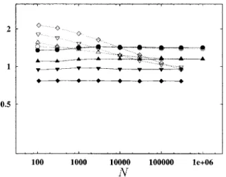
Figure 5 shows a rescaled plot of the scale-free graph’s largest eigenvalue for different values of m. In this figure,1
is compared to the length of the longest row vector
冑
k1 on the ‘‘natural scale’’ of these values, which is冑
mN1/4关11兴. It is clear that if m⬎1 and the system is small, then throughseveral decades共a兲 1is larger than
冑
k1 and共b兲the growth rate of 1 is well below the expected rate of N1/4. In the m⫽1 case, and for large systems,共a兲 the difference between
1 and
冑
k1 vanishes and共b兲the growth rate of the principal eigenvalue will be maximal, too. This crossover in the be- havior of the scale-free graph’s principal eigenvalue is a spe- cific property of sparse growing correlated graphs, and it is a result of the changing level of correlations between the long- est row vectors 共see Sec. VI B兲.3. Comparing the role of the principal eigenvalue in the scale-free graph and the␣Ä1 uncorrelated random
graph: A comparison of structures
Now we will compare the role of the principal eigenvalue in the m⬎1 scale-free graph and the␣⫽1 uncorrelated ran- dom graph through its effect on the moments of the spectral density. On Figs. 4 and 5 one can observe that 共i兲 the prin- cipal eigenvalue of the scale-free graph is detached from the rest of the spectrum, and共ii兲as N→⬁, it grows as N1/4共see also Secs. IV C 2 and VI B兲. It can be also seen that in the limit, the bulk part will be symmetric, and its width will be constant „Fig. 4 rescales this constant width merely by an- other constant, namely关N p(1⫺p)兴⫺1/2. Because of the sym- metry of the bulk part, in the N→⬁ limit, the third moment of 共兲is determined exclusively by the contribution of the principal eigenvalue, which is N⫺1(1)3⬀N⫺1/4. For each moment above the third 共e.g., for the lth moment兲, with growing N, the contribution of the bulk part to this moment will scale as O(1), and the contribution of the principal ei- genvalue will scale as N⫺1⫹l/4. In summary, in the N→⬁
limit, the scale-free graph’s first eigenvalue has a significant contribution to the fourth moment; the fifth and all higher moments are determined exclusively by 1: the lth moment will scale as N⫺1⫹l/4.
In contrast to the above, the principal eigenvalue of the
␣⫽1 uncorrelated random graph converges to the constant pN⫽c in the N→⬁limit, and the width of the bulk part also remains constant 共see Fig. 2兲. Given a fixed number l the contribution of the principal eigenvalue to the lth moment of the spectral density will change as N⫺1clin the N→⬁ limit.
The contribution of the bulk part will scale as O(1), there- fore all even moments of the spectral density will scale as O(1) in the N→⬁limit, and all odd moments will converge to 0.
The difference between the growth rate of the moments of
共兲 in the above two models 共scale-free graph and ␣⫽1 uncorrelated random graph model兲 can be interpreted as a sign of different structure 共see Sec. III A 1兲. In the N→⬁
limit, the average degree of a vertex converges to a constant in both models: limN→⬁具ki典⫽pN⫽c⫽2m. 共Both graphs will have the same number of edges per vertex.兲On the other hand, in the limit all moments of the␣⫽1 uncorrelated ran- dom graph’s spectral density converge to a constant, whereas the moments Ml(l⫽5,6, . . . ) of the scale-free graph’s共兲 will diverge as N⫺1⫹l/4. In other words: the number of loops of length l in the ␣⫽1 uncorrelated random graph will grow as Dl⫽N Ml⫽O(N), whereas for the scale-free graph for every l⭓3, the number of these loops will grow as FIG. 5. Comparison of the length of the longest row vector冑k1
and the principal eigenvalue1in scale-free graphs. Open symbols show1/(冑mN1/4), closed symbols show冑k1/(冑mN1/4). The pa-
rameter values are m⫽1 共䊊兲, m⫽2 共䉭兲, m⫽4 共䉮兲, and m⫽8 共〫兲. Each data point is an average for nine graphs. For the reader’s convenience, data points are connected. If m⬎1 and the network is small, the principal eigenvalue 1 of a scale-free graph is deter- mined by the largest row vectors jointly: the largest eigenvalue is above 冑k1 and the growth rate of1 stays below the maximum possible growth rate, which is1⬀N1/4. If m⫽1, or the network is large, the effect of row vectors other than the longest on1 van- ishes: the principal eigenvalue converges to the length of the long- est row vector, and it grows as1⬀N1/4. Our results show a cross- over in the growth rate of the scale-free model’s principal eigenvalue.
Dl⫽N Ml⫽O(Nl/4). From this we conclude that in the limit, the role of loops is negligible in the␣⫽1 uncorrelated random graph, whereas it is large in the scale-free graph. In fact, the growth rate of the number of loops in the scale-free graph exceeds all polynomial growth rates: the longer the loop size 共l兲 investigated, the higher the growth rate of the number of these loops (Nl/4) will be. Note that the rela- tive number of triangles共i.e., the third moment of the spec- tral density, Ml/N) will disappear in the scale-free graph, if N→⬁.
In summary, the spectrum of the scale-free model converges to a trianglelike shape in the center, and the edges of the bulk part decay slowly. The first eigenvalue is detached from the rest of the spectrum, and it shows an anomalous growth rate. Eigenvalues with large magnitudes belong to eigenvectors localized on vertices with many neighbors. In the present context, the absence of triangles, the high number of loops with length above l⫽3, and the buildup of correlations are the basic properties of the scale- free model.
D. Testing the structure of a ‘‘real-world’’ graph To analyze the structure of a large sparse random graph 共correlated or not兲, here we suggest several tests that can be performed withinO(N) CPU time, useO(N) floating point operations, and can clearly differentiate between the three
‘‘pure’’ types of random graph models treated in Sec. IV.
Furthermore, these tests allow one to quantify the relation between any real-world graph and the three basic types of random graphs.
1. Extremal eigenvalues
In Sec. III A 2 we have already mentioned that the ex- tremal eigenvalues contain useful information on the struc- ture of the graph. As the spectra of uncorrelated random graphs 共Fig. 1兲 and scale-free networks 共Fig. 4兲 show, the principal eigenvalue of random graphs is often detached from the rest of the spectrum. For these two network types, the remaining bulk part of the spectrum, i.e., the set 兵2, . . . ,N其, converges to a symmetric distribution, thus the quantity
Rª1⫺2
2⫺N
共6兲
measures the distance of the first eigenvalue from the main part of 共兲 normalized by the extension of the main part. (R can be connected to the chromatic number of the graph关52兴.兲
Note that in the N→⬁ limit the␣⫽0 sparse uncorrelated random graph’s principal eigenvalue will scale as 具ki典, whereas both2 and兩⫺N兩will scale as 2
冑
具ki典. Therefore, if 具ki典⬎4, the principal eigenvalue will be detached from the bulk part of the spectrum and R will scale as (冑
具ki典⫺2)/4. If, however,具ki典⭐4, 1 will not be detached from the bulk part, it will converge to 0.
The above explanation and Fig. 6 show that in the 具ki典
⬎4 sparse uncorrelated random graph model and the scale- free network,1 and the rest of the spectrum are well sepa- rated, which gives similarly high values for R in small sys- tems. In large systems, R of the sparse uncorrelated random graph converges to a constant, while R in the scale-free model decays as a power-law function of N. The reason for this drop is the increasing denominator on the right-hand side of Eq. 共6兲: 2 and N are the extremal eigenvalues in the lower and upper long tails of共兲, therefore, as N increases, the expectation values of 2 and ⫺N grow as quickly as that of 1. On the other hand, the small-world network shows much lower values of R already for small systems:
here,1is not detached from the rest of the spectrum, which is a consequence of the almost periodical structure of the graph.
On Fig. 6 graphs with the same number of vertices and edges are compared. For large (N⭓10 000) systems and for sparse uncorrelated random graphs R converges to a con- stant, whereas for scale-free graphs and small-world net- works it decays as a power law. The latter two networks significantly differ in the magnitude of R. In summary, the suggested quantity R has been shown to be appropriate for distinguishing between the following graph structures:共i兲pe- riodical or almost periodical 共small world兲,共ii兲uncorrelated nonperiodical, and 共iii兲 strongly correlated nonperiodical 共scale free兲.
2. Inverse participation ratios of extremal eigenpairs Figure 7 shows the inverse participation ratios of the eigenvectors of an uncorrelated random graph, a small-world graph with pr⫽0.01, and a scale-free graph. Even though all FIG. 6. The ratio R⫽(1⫺2)/(2⫺N) for sparse uncorre- lated random graphs 共⫹兲, small-world graphs with pr⫽0.01共䊉兲, and scale-free networks共䉭兲. All graphs have an average degree of 具ki典⫽10, and at each data point, the number of graphs used for averaging was 9. Observe, that for the uncorrelated random graph, R converges to a constant 共see Sec. III A 2兲, whereas it decays rapidly for the two other types of networks, as N→⬁. On the other hand, the latter two network types共small-world and scale-free兲dif- fer significantly in their magnitudes of R.
three graphs have the same number of vertices (N⫽1000) and edges 共5000兲, one can observe rather specific features 共see also the inset of Fig. 7兲.
The uncorrelated random graph’s eigenvectors show very little difference in their level of localization, except for the principal eigenvector, which is much less localized than the other eigenvectors; I(2) and I(N) are almost equal. For the small-world graph’s eigenvectors, I() has many differ- ent plateaus and spikes; the principal eigenvector is not lo- calized, and the second and Nth eigenvectors have high, but different, I() values. The eigenvectors belonging to the scale-free graph’s largest and smallest eigenvalues are local- ized on the ‘‘largest’’ vertices. The long tails of the bulk part of共兲are due to these vertices. All three investigated eigen- vectors (eជ1, eជ2, and eជN) of the scale-free graph are highly localized. Consequently, the inverse participation ratios of the eigenvectors eជ1, eជ2, and eជN are handy for the identifica- tion of the three basic types of random graph models used.
E. Structural variances
Relative variance of the principal eigenvalue for different types of networks: The scale-free graph and self-similarity Figure 8 shows the relative variance of the principal ei- genvalue, i.e., (1)/E(1), for the three basic random graph types.
For nonsparse uncorrelated random graphs (N→⬁ and p⫽const兲this quantity is known to decay at a rate which is faster than exponential 关28,53兴. Comparing sparse graphs with the same number of vertices and edges, one can see that in the sparse uncorrelated random graph and the small-world model the relative variance of the principal eigenvalue drops quickly with growing system size. In the scale-free model, however, the relative variance of the principal eigenvalue’s distribution remains constant with an increasing number of vertices.
In fractals, fluctuations do not disappear as the size of the system is increased, while in the scale-free graph, the relative variance of the principal eigenvalue is independent of system size. In this sense, the scale-free graph resembles self-similar systems.
V. CONCLUSIONS
We have performed a detailed analysis of the complete spectra, eigenvalues, and the eigenvectors’ inverse participa- tion ratios in three types of sparse random graphs: the sparse uncorrelated random graph, the small-world model, and the scale-free network. Connecting the topological features of these graphs to algebraic quantities, we have demonstrated that 共i兲the semi circle law is not universal, not even for the uncorrelated random graph model;共ii兲the small-world graph is inherently noncorrelated and contains a high number of FIG. 7. Main panel: Inverse participation ratios of the eigenvec-
tors of three graphs shown as a function of the corresponding ei- genvalues: uncorrelated random graph共⫹兲, small-world graph with pr⫽0.01共䊉兲, and scale-free graph 共䉭兲. All three graphs have N
⫽1000 vertices, and the average degree of a vertex is 具ki典⫽10.
Observe that the eigenvectors of the sparse uncorrelated random graph and the small-world network are usually nonlocalized关I() is close to 1/N兴. On the contrary, eigenvectors belonging to the scale-free graph’s extremal eigenvalues are highly localized with I() approaching 0.1. Note also that for⬇0, the scale-free graph’s I() has a significant ‘‘spike’’ indicating again the localization of eigenvectors. Inset: Inverse participation ratios of the first, second, and Nth eigenvectors of an uncorrelated random graph共⫹兲, a small- world graph with pr⫽0.01 共䊉兲, and a scale-free graph 共䉭兲. For each data point, the number of vertices was N⫽300 000 and the number of edges was 1 500 000. Clearly, the principal eigenvector of the scale-free graph is localized, while the principal eigenvector of the other two systems共the uncorrelated models兲is not. Note also that the inverse participation ratios of the second and Nth eigenvec- tors clearly differ in the small-world graph—the spectrum of this graph has already been shown to be strongly asymmetric—whereas in the uncorrelated random graph the inverse participation ratios of eជ2 and eជN are approximately the same. Thus, with the help of the inverse participation ratios of eជ1, eជ2, and eជN, one can identify the three main types of random graphs used here.
FIG. 8. Size dependence of the relative variance of the principal eigenvalue, i.e., (1)/E(1), for sparse uncorrelated random graphs 共⫹兲, small-world graphs with pr⫽0.01共䊉兲, and scale-free graphs共䉭兲. The average degree of a vertex is具ki典⫽10, and 1000 graphs were used for averaging at every point. Observe that in the uncorrelated random graph and the small-world model
(1)/E(1) decays with increasing system size; however, for scale-free graphs with the same number of edges and vertices, it remains constant.
triangles;共iii兲the spectral density of the scale-free graph is made up of three, well distinguishable parts 共center, tails of bulk, first eigenvalue兲, and as N→⬁, triangles become neg- ligible and the level of correlations changes.
We have presented practical tools for the identification of the above-mentioned basic types of random graphs and fur- ther, for the classification of real-world graphs. The robust eigenvector techniques and observations outlined in this pa- per combined with previous studies are likely to improve our understanding of large sparse correlated random structures.
Examples for algebraic techniques already in use for large sparse correlated random structures are analyses of the Inter- net 关6,18兴and search engines关54,62兴and mappings关55,56兴 of the World-Wide Web. Besides the improvement of these techniques, the present work may turn out to be useful for analyzing the correlation structure of the transactions be- tween a very high number of economical and financial units, which has already been started in, e.g., Refs.关57–59兴. Lastly, we hope to have provided quantitative tools for the classifi- cation of further ‘‘real-world’’ networks, e.g., social and bio- logical networks.
Note added in proof. Recently, we were made aware of a manuscript by Goh, Kahng, and Kim 关63兴investigating the spectral properties of scale-free networks. Also, our attention has been drawn to a recent publication of Bauer and Golinelli关64兴on the spectral properties of uncorrelated ran- dom graphs.
ACKNOWLEDGMENTS
We thank D. Petz, G. Stoyan, G. Tusna´dy, K. Wu, and B.
Kahng for helpful discussions and suggestions. This research was partially supported by a HNSF Grant No. OTKA T033104 and NSF Grant No. PHY-9988674.
APPENDIX A: THE SPECTRUM OF A SMALL-WORLD GRAPH FOR prÄ0 REWIRING PROBABILITY
1. Derivation of the spectral density
If the rewiring probability of a small-world graph is pr
⫽0, then the graph is regular, each vertex is connected to its
k nearest neighbors, and the eigenvalues can be computed using the graph’s symmetry operations. Rotational symmetry operations can be easily recognized, if the vertices of the graph are drawn along the perimeter of a circle 共see Fig. 9兲: let P(n) (n⫽0,1, . . . ,N⫺1) denote the symmetry operation that rotates the graph by n vertices in the anticlockwise di- rection. Being a symmetry operation, each P(n) commutes with the adjacency matrix A, and they have a common full orthogonal system of eigenvectors.
Now, we will create a full orthogonal basis of A.共We will treat only the case when N is an even number; odd N’s can be treated similarly.兲It is known that the eigenvalues of A are real; however, to simplify calculations, we will use complex numbers first. The eigenvectors of every P(n) are eជ1,eជ2, . . . ,eជN,
共el兲j⫽exp
冉
2iNjl冊
, 共A1兲where l⫽0,2, . . . ,N⫺1 and i⫽
冑
⫺1. The eigenvalue of P(n) on eជlissl(n)⫽exp
冉
2inlN冊
. 共A2兲By adding these values pairwise, one can obtain the N eigenvalues of the graph
l⫽2
兺
j⫽1 k/2cos
冉
2jlN冊
. 共A3兲In the previous exponential form the right-hand side is a summation for a geometrical series; therefore,
l⫽sin关共k⫹1兲l/N兴
sin共l/N兲 ⫺1. 共A4兲 In the N→⬁ limit, this converges to
共x兲⫽sin关共k⫹1兲x兴
sin共x兲 ⫺1, 共A5兲 where x is evenly distributed in the interval关0,兴.
2. Singularities of the spectral density
The spectral density is singular in⫽(x), if and only if (d/dx)(x)⫽0, which is equivalent to
共k⫹1兲tan共x兲⫽tan关共k⫹1兲x兴. 共A6兲 Since k is an even number, both this equation and Eq.
共A5兲are invariant under the transformation x哫⫺x, there- fore only the x⑀关0,/2兴 solutions will give different val- ues. If k⫽10共see Fig. 3兲, Eq.共A6兲has k/2⫹1⫽6 solutions in 关0,/2兴, which are x⫽0, 0.410, 0.704, 0.994, 1.28, and
/2. Therefore, according to Eq.共A5兲, in the N→⬁ limit the spectral density will be singular in the following points:
i⫽⫺3.46,⫺2.19,⫺2,0.043,0.536, and k⫽10. 共A7兲 FIG. 9. The regular ring graph obtained from the small-world
model in the pr⫽0 case: rotations ( P(n) for every n⫽0,1, . . . ,N
⫺1) are symmetry operations of the graph. The P(n) operators 共there are N of them兲can be used to create a full orthogonal basis of the adjacency matrix A: taking any P(n), it commutes with A, there- fore they have a common full orthogonal system of eigenvectors.
共For a clear illustration of symmetries, this figure shows a graph with only N⫽15 vertices and k⫽4 connections per vertex.兲
APPENDIX B: CROSSOVER IN THE GROWTH RATE OF THE SCALE-FREE GRAPH’S
PRINCIPAL EIGENVALUE
The largest eigenvalue is influenced only by the longest row vector if and only if the two longest row vectors are almost orthogonal:
vជ1vជ2Ⰶ兩vជ1兩兩vជ2兩. 共B1兲
For m⬎1, the left-hand side共lhs兲of Eq.共B1兲is the num- ber of simultaneous 1’s in the two longest row vectors, and the rhs can be approximated with 兩vជ1兩2⫽k1, the largest de- gree of the graph. It is known关11兴that for large j ( j⬎i), the
jth vertex will be connected to vertex i with probability Pi j
⫽m/(2
冑
i j ). Thus, we can write Eq. 共B1兲 in the following forms:t
兺
⫽1 NP1t2Ⰶt
兺
⫽1 NP1t 共B2兲
or
冑
Ncln NcⰇm
4 , 共B3兲
where Ncis the critical system size.
关1兴P. Erdo˝s and A. Re´nyi, Publ Math 6, 290共1959兲; Publ. Math.
Inst. Hung. Acad. Sci. 5, 17共1960兲; 5, 290共1959兲; Acta Math.
Acad. Sci. Hung. 12, 261共1961兲.
关2兴B. Bolloba´s, Random Graphs共Academic, London, 1985兲. 关3兴S. Redner, Eur. Phys. J. B 4, 131共1998兲.
关4兴D.J. Watts and S.H. Strogatz, Nature 共London兲 393, 440 共1998兲.
关5兴D.J. Watts, Small Worlds: The Dynamics of Networks Between Order and Randomness (Princeton Reviews in Complexity) 共Princeton University Press, Princeton, NJ, 1999兲.
关6兴M. Faloutsos, P. Faloutsos, and C. Faloutsos, Comput. Com- mun. Rev. 29, 251共1999兲.
关7兴L.A. Adamic and B.A. Huberman, Nature共London兲401, 131 共1999兲.
关8兴R. Albert, H. Jeong, and A.-L. Baraba´si, Nature共London兲401, 130共1999兲.
关9兴H. Jeong, B. Tombor, R. Albert, Z.N. Oltvai, and A.-L. Bara- ba´si, Nature共London兲407, 651共2000兲.
关10兴A.-L. Baraba´si and R. Albert, Science 286, 509共1999兲. 关11兴A.-L. Baraba´si, R. Albert, and H. Jeong, Physica A 272, 173
共1999兲.
关12兴L.A.N. Amaral, A. Scala, M. Barthe´le´my, and H.E. Stanley, e-print cond-mat/0001458.
关13兴A.L. Baraba´si, H. Jeong, E. Ravasz, Z. Ne´da, T. Vicsek, and A.
Schubert共unpublished兲.
关14兴M.E.J. Newman, Proc. Natl. Acad. Sci. USA 98, 404共2001兲;e- print cond-mat/0011144.
关15兴A. Medina, I. Matta, and J. Byers, Comput Commun. Rev. 30, 18共2000兲.
关16兴R. Cohen, K. Erez, D. ben-Avraham and S. Havlin, Phys. Rev.
Lett. 85, 4626共2000兲.
关17兴R. Cohen, K. Erez, D. ben-Avraham, and S. Havlin, Phys. Rev.
Lett. 86, 3682共2001兲.
关18兴A. Broder, R. Kumar, F. Maghoul, P. Raghavan, S. Rajalopa- gan, R. Stata, A. Tomkins, and J. Wiener, in Proceeding of the 9th International World-Wide Web Conference, 2000 共un published兲, see 共http://www.almaden.ibm.com/cs/k53/
www9.final/兲.
关19兴Petra M. Gleiss, Peter F. Stadler, Andreas Wagner, and David A. Fell共unpublished兲.
关20兴M.L. Mehta, Random Matrices, 2nd ed.共Academic, New York, 1991兲.
关21兴A. Crisanti, G. Paladin, and A. Vulpiani, Products of Random Matrices in Statistical Physics, Springer Series in Solid-State Sciences Vol. 104共Springer, Berlin, 1993兲.
关22兴E.P. Wigner, Ann. Math. 62, 548 共1955兲; 65, 203共1957兲; 67, 325共1958兲.
关23兴F. Hiai and D. Petz The Semicircle Law, Free Random Vari- ables and Entropy 共American Mathematical Society, Provi- dence, 2000兲, Section 4.1.
关24兴F.J. Dyson, J. Math. Phys. 3, 140共1962兲. 关25兴E.P. Wigner, SIAM Rev. 9, 1共1967兲.
关26兴T. Guhr, A. Mu¨ller-Groeling, and H.A. Weidenmu˝ller, Phys.
Rep. 299, 189共1998兲.
关27兴F. Juha´sz, in Algebraic Methods in Graph Theory共North Hol- land, Amsterdam, 1981兲, pp. 313–316.
关28兴D. Cvetkovic and P. Rowlinson, Linear Multilinear Algebra 28, 3共1990兲.
关29兴B.V. Bronx, J. Math. Phys. 5, 215共1964兲.
关30兴M.E.J. Newman, C. Moore, and D.J. Watts, Phys. Rev. Lett.
84, 3201共2000兲.
关31兴The number of edges meeting at one vertex of a graph is called the degree of that vertex, and a graph is called regular if every vertex has the same degree.
关32兴P.L. Krapivsky and S. Redner, e-print cond-mat/0011094.
关33兴P.L. Krapivsky, G.J. Rodgers, and S. Redner, e-print cond-mat/0012181.
关34兴S.N. Dorogovtsev and J.F.F. Mendes, Phys. Rev. E 62, 1842 共2000兲.
关35兴S.N. Dorogovtsev, J.F.F. Mendes, and A.N. Samukhin, e-print cond-mat/0011077.
关36兴S.N. Dorogovtsev and J.F.F. Mendes, Phys. Rev. E 63, 056125 共2001兲.
关37兴R. Albert and A.-L. Baraba´si, Phys. Rev. Lett. 85, 5234共2000兲. 关38兴G. Bianconi and A.-L. Baraba´si, e-print cond-mat/0011224.
关39兴G. Bianconi, and A.-L. Baraba´si, e-print cond-mat/0011029.
关40兴A. Vazquez, e-print cond-mat/0006132.
关41兴J.M. Montoya and R.V. Sole´共unpublished兲; R.V. Sole´ and J.
M. Montoya共unpublished兲.
关42兴Handbook of Combinatorics, edited by R.L. Graham, M.
Gro¨tschel, and L. Lova´sz共North-Holland, Amsterdam, 1995兲. 关43兴D. M. Cvetkovic´, M. Doob, and H. Sachs, Spectra of Graphs
共VEB Deutscher Verlag der Wissenschaften, Berlin, 1980兲. 关44兴W.H. Press, S.A. Teukolsky, W.T. Vetterling, and B.P. Flan-