Supplemental material for
Quantum graphs whose spectra mimic the zeros of the Riemann zeta function
Jack Kuipers, Quirin Hummel, and Klaus Richter
Institut f¨ur Theoretische Physik, Universit¨at Regensburg, D-93040 Regensburg, Germany
Appendix A: The density of Riemann zeta zeros in the complex plane
Taking the logarithmic derivativeζ′(z)/ζ(z) of the Rie- mann zeta function transforms its zeros into single poles in the complex plane. Therefore its real part evaluated at the critical line,z= 1/2+it−τin the limitτ→0−, gives Dirac-delta peaks at all the non-trivial zeros, assuming they indeed lie on the critical line z = 1/2 + it. The divergent expression (2) of the Letter for the oscillating part of the density of the Riemann zeros corresponds to Re[(ζ′/ζ)(1/2+it)]/πusing the Euler product representa- tion ofζand ignoring the fact that this only converges for Rez >1. Smoothing expression (2) of the Letter with a Gaussian finally makes it convergent and transforms the delta peaks into Gaussian peaks of finite width.
In order to visualize the density of Riemann zeros in the complex plane we define
doscC (t+ iτ) =−1 π
X
p
∞
X
m=1
lnp
pm/2exp (−itmlnp+τ mlnp) (A1) on the half plane τ ≤ 0 to the right of the critical line, which equals (ζ′/ζ)(1/2 + it−τ)/π using the divergent series expansion ofζ(z).
To achieve convergence forτ ∈[−1/2,0], we smooth it parallel to the critical line by convolving it with a Gaus- sian with respect to t. For the left side τ > 0 of the critical line we apply the reflection property of the ζ- function
ζ(1−z) = 2(2π)−zcosπz 2
Γ(z)ζ(z) (A2) onζ′/ζ= (lnζ)′ to define
doscC (t+ iτ) =−[doscC (t−iτ)]∗−2 ¯dC(t+ iτ), (A3) which relates it back to the density evaluated at τ <0 using (A1). ¯dCis defined as
d¯C(t+ iτ) =− 1
2πln 2π−1 4cotπ
4 +π
2(it−τ) + 1
2πψ 1
2−it+τ
, (A4)
where ψ(z) denotes the digamma function [forτ = 0, it corresponds to the smooth part (1) of the Letter].
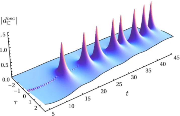
FigureA1shows the absolute value ofdoscC (t+ iτ) with a truncation to 10000 primes and a smoothing width of 0.3, whereas Fig. A2 shows the real part of the same object. The pole-like peaks at the non-trivial Riemann zeta zeros can easily be identified.
FIG. A1. Absolute value|doscC (t+ iτ)|. The first 10000 primes have been used and a smoothing int-direction with a Gaussian of standard deviation 0.3 has been applied.
FIG. A2. Real part Re[doscC (t+ iτ)]. The first 10000 primes have been used and a smoothing int-direction with a Gaussian of standard deviation 0.3 has been applied.
Appendix B: Increasing the number of copies of butterfly graphs
If from the start we set the number of copies of the butterfly graphs tolp,m =mthen the corresponding re- cursion
cos(θp,m) =− 1 2m2pm/2−
d<m
X
d|m
d m
2 cosm
dθp,d
(B1)
2
0 10 20 30 40
-0.5 0.0 0.5 1.0
k dΕosc HkL
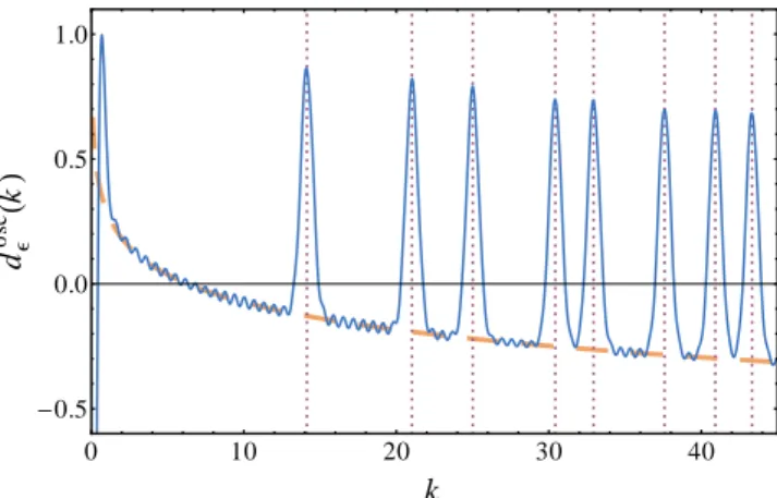
FIG. B1. Solid blue: density of exact eigenvalues of the lin- early growing set of butterfly graphs (B1) smoothed with a Gaussian of width ǫ = 0.4 and the mean part subtracted.
The set of graphs is truncated atǫmlnp≤3.7. Dotted pur- ple: exact zeros of the Riemann zeta function. Dashed orange:
negative of the mean part of the Riemann zeros density.
is solvable with real θp,m for all (p, m) since the sum of squared divisors of m(divided by m2) is bounded suffi- ciently. One can estimate
d<m
X
d|m
d2 m2 ≤
⌊√ m⌋
X
d|m
d2 m2 +
⌊√ m⌋
X
d|m
1
d2 −1 (B2)
< 1 3√m+ 1
2m+ 1
6m3/2 +π2
6 −1≡B(m). For m ≥ 4 the bound B(m) is already smaller than 1 [B(4) = 0.957. . .] and the additional summand in (B1) is 1/(2m2pm/2) ≤1/128. Thus for allm ≥ 4 the RHS of (B1) is smaller than 1 in absolute value. The cases m = 1,2,3 can be easily checked by direct calculation of the sum of squares of divisors. They give sufficient bounds for (B1) for the worst case p= 2 and hence for all primesp. Therefore, the recursion (B1) has solutions for all (p, m). Figure B1 shows the fluctuating part of the exact spectrum of a truncated set of butterfly graphs with linearly growing number of copies lp,m = m. The enhancement of the small damped high frequency oscilla- tions in comparison to the butterfly graphs without linear growth in Fig. 2 of the Letter is a direct consequence of the increased weight of butterflies with longer bonds.
Appendix C: Sets of butterfly graphs with identical lengths
The prescriptions (14) of the Letter and (B1) allow us to construct a sets of graphs with the same oscillating part of the density of states as the Riemann zeros, but rely on a recursive construction to find the graphs. If we
FIG. C1. Settingp = 2 and R = 30 we calculate the shift
∆2,r from equally spaced angles as defined in (C11). The dotted line is from the exact numerical solution of the 30 simultaneous equations in (C4) while the solid line is derived from the approximate solutions of (C9).
perform the sum overm in Eq. (2) of the Letter to get dosc(t) =−1
π X
p
lnp
√pcos(tlnp)−1
p+ 1−2√pcos(tlnp), (C1) the resultant terms
doscp (k) =−lnp π
√pcos(klnp)−1
p+ 1−2√pcos(klnp) (C2) are periodic with period 2π/ln(p). This is the same pe- riod as the solutions with m = 1 before. A butterfly graph of bond length ln(p) contributes to dosc(k) with this period (and also all fractions of it; the amplitudes of all the harmonics are determined by the scattering ma- trix). Thus a set of butterfly graphs, all with bond length ln(p) could be constructed in a way that together they produce the correct Fourier coefficients of doscp (k). We can try to find this set of butterfly graphs for each prime pso that together they again give Eq. (2) of the Letter.
If we label the scattering matrices of all the butterflies Sp,r, they have to fulfill the equations
X
r
TrSp,rm =− 1
pm/2, (C3)
or
2X
r
cos(mθp,r) =− 1
pm/2, (C4) in terms of the positiveθp,r< π.
1. Approximate solution
With a finite set of graphsr= 1, . . . , Rwe can find nu- merical solutions for the firstRequations formin (C4), but more importantly we can find approximate solutions
3 for any number of graphs. Assume our discrete pairs of
solutions −π < ±θp,r < π follow a density ψp(θ) then the limit of infinite solutions would be
2 Z π
0
cos(mθ)ψp(θ)dθ=− 1
pm/2 (C5) for eachm. Solving forψpis just taking the Fourier series so
πψp(θ) =−X
m
cos(mθ)
pm/2 = 1−√pcos(θ)
p+ 1−2√pcos(θ), (C6) exactly mimicking (C1).
WithRpairs of θsolutions, the overall density should beψp(θ) +R/πand we want discrete solutions that best approximate this density. Dividing the overall density be- tweenθ=−πandθ=πinto 2Rbars of equal (unit) area, we could expect to find a solution inside each bar and we approximate by placing it at the center of mass. Equiv- alently we are dividing the cumulative function evenly.
From the symmetry, we only need to look at the solu- tions between 0 andπwhich should then satisfy
r−1
2 =Rθp,r
π +
Z θp,r
0
ψp(θ)dθ , (C7) with
π Z θp,r
0
ψp(θ)dθ=−Im X∞ m=1
eimθp,r mpm/2
= Imh ln
1−p−1/2eiθp,ri . (C8) Since the argument of the logarithm in (C8) always lies in the right half plane ofC, we can write
πr−π
2 =Rθp,r+ arctan sinθp,r
cosθp,r−√p, (C9) or equivalently
tan(π∆p,r) = sinθp,r
√p−cosθp,r
, (C10)
with−1/2<∆p,r <1/2, where we defined the shift from equally spaced angles as
∆p,r =Rθp,r
π −r+1
2. (C11)
2. Examples
ForR= 30 we plot the shifts (C11) forp= 2 for both the exact solutions of the 30 equations in (C4) as well as the approximate solutions from (C9) or (C10) in Fig.C1.
At the level of the accuracy visible in the graph, these shifts are essentially identical.
Taking a larger number of approximate solutions by setting R = 100 we place a Gaussian smoothed delta
FIG. C2. The solid line is the density of states of 100 butterfly graphs of length ln(2) smoothed by a Gaussian function of width w=π/10 and with the mean part 100/πsubtracted.
The dotted line instead is thep= 2 term of Eq. (C1) of the Letter, transformed to θ = kln(2) and smoothed with the same Gaussian.
0 10 20 30 40
-0.5 0.0 0.5 1.0
k dΕosc HkL
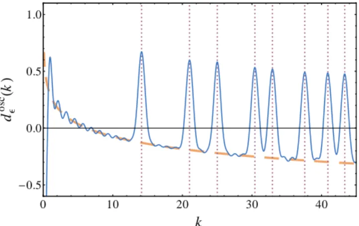
FIG. C3. Solid blue: density of eigenvalues of the set of but- terfly graphs involving identical bond lengths for each prime up to p = 181 derived using (C10) and the low value of R = 10. The result is smoothed with a Gaussian of width ǫ= 0.5 and the mean part has been subtracted. Dotted pur- ple: exact zeros of the Riemann zeta function. Dashed orange:
negative of the smooth part of the Riemann zeros density.
function (of width ǫ = π/10) on each of the ±θ2,r and their periodic repetitions and subtract the mean part 100/π. Plotting the result as the solid line in Fig. C2 we can compare to the (equally smoothed) p= 2 term of (C1). In terms of anglesθ=kln(2) this is just the con- volution ofψ2(θ) with the same Gaussian and we overlay this result as a dotted line in Fig. C2. Again the lines are indistinguishable in the graph.
Even a small set of graphs is enough to be able to pick out the zeros of the Riemann zeta function. Setting R= 10 for example, we plot in Fig.C3the smoothed os- cillating partdoscǫ (k) of a complete set of butterfly graphs with equal bond lengths ln(p) for primes up to 181. The spectrum corresponds to the approximate solutions us- ing (C10).