The composite size spectra (Fig

1 RESOLUTION OF COMPOSITE AND COMBINED SIZE SPECTRA OF PHYTO- AND PROTOZOOPLANKTON

Compositesize spectra of maximum resolution can be constructed when individual size spectra of every taxonomic group are added up, i.e.j represents all taxonomic groups present in the dataset. All taxon- specific KDEs can be assembled to a composite size spectrum, for example of all phytoplankton or zooplankton taxa:

KDE^composite_phy/zoo (s) =

M_phy/zoo

X

j=1

KDE_j(s, h_j) (S1)

Here, the bandwidth parameterh_j is taxon-specific. The variability in size is typically smaller within taxa than in combined phytoplankton and microzooplankton subsets, which results in a smaller degree of smoothing (see equation 5), and thus a higher resolution incompositespectra, as compared tocombined spectra.

The composite size spectra (Fig. S1, left panels) therefore exhibit details with the highest possible resolution of the communities’ size structure. The high level of detail in the composite size spectra turned out to be associated with considerable uncertainties, with many narrow peaks, in particular for ESD>20 µm. The abundance of cells of ESD<20 µm seemed less variable among taxa. The highest abundance in phytoplankton appeared in the proximity of 5 µm and also around ESD = 7 µm. These were mainly diatoms and prymnesiophytes. Likewise, the highest abundance of heterotrophs fell into the same size range. It is noteworthy that the distinct peaks around ESD = 5 µm and ESD = 7 µm were also apparent in the spectra of heterotrophic cells, but with an additional distinct peak in the proximity of 10–11 µm.

Furthermore, heterotrophic dinoflagellates lead to an additional peak at ESD = 200 µm.

Considering the confidence limits, it appeared difficult to unambiguously interpret ecological details of thecompositesize spectra. We found major characteristics of thecompositesize spectra to be well and consistently captured by thecombinedsize spectra (Fig. S1, right panels). Similar to thecompositesize spectra, autotrophic and heterotrophiccombinedspectra overlapped between ESD≈20 µm and ESD≈ 50 µm. In size ranges ESD>50 µm, where cell abundance decreased significantly,combinedandcomposite size spectra differed. The largest phytoplankton in thecompositespectrum was larger than ESD = 200 µm, while thecombined spectrumapproximated 1 cell L⁻¹s⁻¹at ESD≈180 µm. Furthermore, a symmetrical peak was centred around 110 µm in thecombinedspectrum and corresponded an trough in thecomposite spectrum, where in turn a peak followed around ESD≈140 µm. Heterotrophic cells covered approximately the same size range in thecompositeandcombinedspectra.

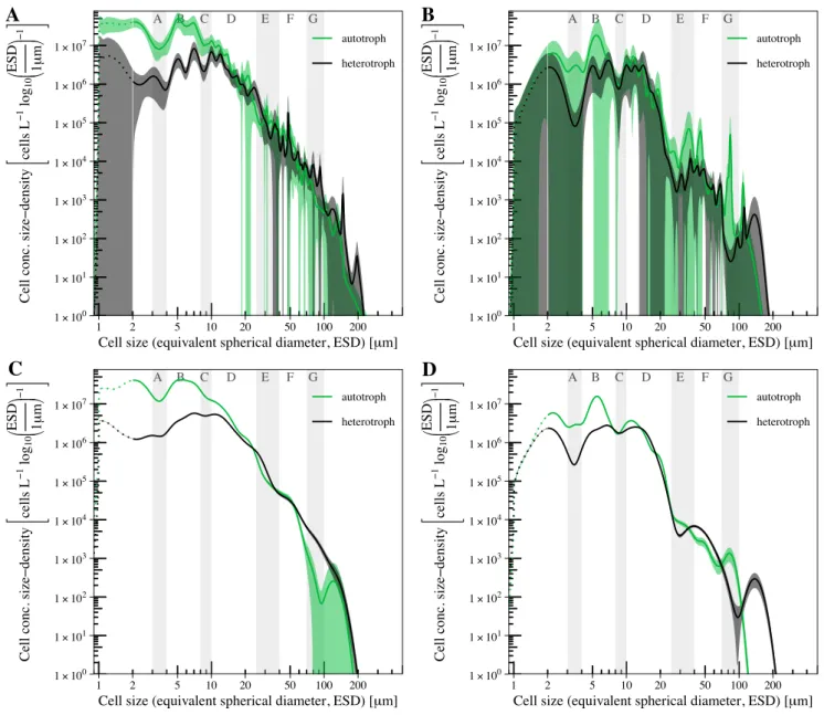
Analogously, the analysis ofcompositeseasonally separated size spectra (Fig.S2AandB) gave no clear advantage over thecombined spectra (Fig. S2CandD). Many details in thecompositesize spectra are subject to considerable uncertainty, which complicates the identification and interpretation of general trends, if compared to patterns derived with thecombined spectra. For instance, the comparison between summer (left panels of Fig. S2) and autumn spectra (right panels) illustrates that thecombinedsize spectra show only a few peaks and troughs, but total cell concentration are still in accordance with thecomposite

A B C D E F G

A B C D E F G

A B C D E F G

A B C D E F G

composite combined

autotrophheterotroph

1 2 5 10 20 50 100 200 1 2 5 10 20 50 100 200

1×10⁰ 1×10¹ 1×10² 1×10³ 1×10⁴ 1×10⁵ 1×10⁶ 1×10⁷

1×10⁰ 1×10¹ 1×10² 1×10³ 1×10⁴ 1×10⁵ 1×10⁶ 1×10⁷

Cell size (equivalent spherical diameter, ESD) [µm]

Cell conc. size−density  cells L−1 log10 ESD 1µm −1 

autotroph heterotroph

Figure S1. Composite(left) andcombined (right) size spectra for autotrophic (upper) and heterotrophic (lower) microplankton.

spectra. Important and predominant features, e.g. the depression around 4 µm, the step-like drop around 30 µm, and the trough in summer and the peak in autumn of the autotrophic size spectra at 90 µm, remain well expressed in thecombined size spectra, which also confirms the consistency and robustness of our approach.

A B C D E F G

1×10⁰ 1×10¹ 1×10² 1×10³ 1×10⁴ 1×10⁵ 1×10⁶ 1×10⁷

1 2 5 10 20 50 100 200

Cell size (equivalent spherical diameter, ESD) [μm]

Cell conc. size−density ⎡ ⎣⎢cellsL−1log10⎛ ⎝⎜ESD 1μm⎞ ⎠⎟−1⎤ ⎦⎥

autotroph heterotroph

A A B C D E F G

1×10⁰ 1×10¹ 1×10² 1×10³ 1×10⁴ 1×10⁵ 1×10⁶ 1×10⁷

1 2 5 10 20 50 100 200

Cell size (equivalent spherical diameter, ESD) [μm]

Cell conc. size−density ⎡ ⎣⎢cellsL−1 log10⎛ ⎝⎜ESD 1μm⎞ ⎠⎟−1⎤ ⎦⎥

autotroph heterotroph

B

A B C D E F G

1×10⁰ 1×10¹ 1×10² 1×10³ 1×10⁴ 1×10⁵ 1×10⁶ 1×10⁷

1 2 5 10 20 50 100 200

Cell size (equivalent spherical diameter, ESD) [μm]

Cell conc. size−density ⎡ ⎣⎢cellsL−1log10⎛ ⎝⎜ESD 1μm⎞ ⎠⎟−1⎤ ⎦⎥

autotroph heterotroph

C _{A B C D E F G}

1×10⁰ 1×10¹ 1×10² 1×10³ 1×10⁴ 1×10⁵ 1×10⁶ 1×10⁷

1 2 5 10 20 50 100 200

Cell size (equivalent spherical diameter, ESD) [μm]

Cell conc. size−density ⎡ ⎣⎢cellsL−1 log10⎛ ⎝⎜ESD 1μm⎞ ⎠⎟−1⎤ ⎦⎥

autotroph heterotroph

D

Figure S2. Compositesize spectra for summer (A) and autumn (B). Species-specific size spectra were summed to autotrophic and heterotrophic spectra and averaged across samples;Combinedsize spectra for summer (C) and autumn (D), derived from a combined data-set of all available data. Shaded areas mark the confidence interval (KDE(s)±1.96×SE(s)).

2 SUPPLEMENTARY TABLES AND FIGURES

3.2 % 5.8 % 3.5 % 2.1 %

1.1 % 0.1 % < 0.1 % 0.1 %

5.4 % 0.6 % 1.1 % 3.9 %

14.1 %

39.6 % 36.6 % 17.6 % 30.4 %

27.7 % 48.8 %

< 0.1 % < 0.1 %

1.1 % < 0.1 % 5.9 % 0.4 %

1.1 %

< 0.1 % < 0.1 % < 0.1 % < 0.1 %

0.9 % < 0.1 % 1.2 % 0.2 %

< 0.1 % < 0.1 % < 0.1 % 0.1 %

0.1 % < 0.1 % < 0.1 % 0.1 %

0.3 % 3 % 0.4 % 0.8 %

< 0.1 % 0.2 % 0.4 %

< 0.1 % < 0.1 %

< 0.1 % < 0.1 % 0.4 %

0.4 % 0.2 % 0.2 %

< 0.1 % < 0.1 %

0.4 % 0.3 % 0.3 % 0.1 %

< 0.1 %

1.1 % 1.6 % 0.9 % 0.3 % < 0.1 %

5.9 % 1.7 % 0.7 % 1.3 %

< 0.1 %

1.6 % 1.2 % 3.8 % 2 %

1.6 % 0.4 % 0.4 %

0.2 % 0.8 % < 0.1 % < 0.1 %

10.8 % 25.7 % 1.8 % 1.3 %

5.8 % 0.1 %

5.6 % 7.5 % 1.1 % 1.4 %

< 0.1 % < 0.1 % < 0.1 %

19.1 % 13 % 3.2 % 3.3 %

0.1 % 0.2 %

0.6 % 0.4 % 0.1 %

1.1 % < 0.1 %

0.5 %

0.2 % < 0.1 % < 0.1 % 0.1 %

< 0.1 % 0.3 % 0.1 %

0.2 %

2.2 % 0.1 % 6.4 % 1.8 %

0.2 % < 0.1 % < 0.1 %

< 0.1 % < 0.1 % < 0.1 % < 0.1 %

< 0.1 % < 0.1 % < 0.1 % < 0.1 %

< 0.1 % < 0.1 %

< 0.1 % < 0.1 %

< 0.1 % < 0.1 %

0.2 % < 0.1 % Summer,

Atlantic S1

Summer, Polar

S2 Autumn,

Atlantic S3

Autumn, Polar

S4 Phaeocystis sp.

Phaeocystis pouchetiiEmiliania huxleyi Coccolithus pelagicusCoccolithophores

Micromonas spp.

Thalassiosira spp.Rhizosolenia spp.Melosira arcticaProboscia alataGuinardia sp.

Eucampia groenlandicaCorethron sp.

Chaetoceros spp. (spore)Chaetoceros spp.Centric Diatoms

Pseudo−nitzschia spp.

Pleurosigma/Gyrosigma spp.Nitzschia cf seriata (chain)Fragilariopsis oceanicaNavicula vanhoeffeniiFragilariopsis spp.Navicula pelagicaPennate DiatomsNitzschia spp.Navicula spp.Haslea spp.

Fragilariopsis cylindrus (chain)Cylindrotheca closteriumFossula arcticaFragilaria sp.

Cryptophytes Dinobryon sp.

Dictyocha speculum MicroflagellatesFlagellates

Protoperidinium spp.Prorocentrum sp.

Prorocentrum cf minimumH. thecate DinoflagellatesA. thecate DinoflagellatesCeratium arcticumH. DinoflagellatesA. DinoflagellatesAmphidinium spp.

Mesodinium rubrumFavella sp.Ciliates Monosiga sp.

ChoanoflagellatesBicosta sp.

Tintinnids Stenosemella sp.Parafavella sp.Ptychocylis sp.

Parafavella denticulataAcanthostomella sp.

Acanthostomella norvegica

Eutreptiella spp.

Undefined species

1 10² 10⁴ 10⁶ 10⁸

Cell concentration [cells L⁻¹]

0.6 % 2.4 % 4.5 % 2.9 %

1.6 % 0.2 % < 0.1 % 0.2 %

1 % 0.3 % 2 % 3.5 %

0.9 %

1.4 % 7.9 % 1.9 % 13 %

0.1 % 0.2 %

0.3 % 0.1 %

0.8 % 0.4 % 16.3 % 3.4 %

0.6 %

0.6 % 0.4 % < 0.1 % 0.1 %

2.6 % 0.1 % 3.4 % 5.7 %

< 0.1 % < 0.1 % 0.1 % 2.4 %

3.5 % 0.7 % 0.2 % 0.9 %

6.5 % 8.9 % 6.2 % 4.3 %

< 0.1 % 0.1 % 0.1 %

0.4 % < 0.1 %

< 0.1 % < 0.1 % 0.9 %

0.7 % 0.3 % 0.1 %

< 0.1 % 0.1 %

1.1 % 0.5 % 0.5 % 0.4 %

1.1 %

0.1 % 0.3 % 0.5 % 0.1 % < 0.1 %

0.1 % 0.3 % 0.1 % 0.1 %

< 0.1 %

0.8 % 0.4 % 1.9 % 1.1 %

4.2 % 1.1 % 0.4 %

2.6 % 4.3 % 0.4 % 0.1 %

1.2 % 2.6 % 1.1 % 0.5 %

0.2 % 0.1 %

27.7 % 22.3 % 9.7 % 12.8 %

< 0.1 % 0.1 % < 0.1 %

17.8 % 40 % 25.4 % 28.7 %

1.2 % 0.5 %

2.8 %4 % 0.2 %

1.5 % 0.2 %

4.9 %

19.4 % 1.6 % 4.4 %

2 % 0.2 %

1.7 % 7.4 %

0.3 %

0.3 % < 0.1 % < 0.1 % 0.5 %

0.2 % 0.3 % 0.6 %

2.3 % 0.8 % 1.1 % 0.1 %

6.7 % 0.5 % 0.6 % 1.4 %

0.1 % < 0.1 %

0.5 % 0.9 %

0.7 % 0.6 %

0.8 % 0.1 %

Prymnesiophytes

Chlorophytes

Centric Diatoms

Pennate Diatoms

Cryptophytes Chrysophytes Silicoflagellates Flagellates

Dinoflagellates

Ciliates

Choanoflagellates

Tintinnids

Euglenophytes Undefined Summer,

Atlantic S1

Summer, Polar

S2 Autumn,

Atlantic S3

Autumn, Polar

S4

0.1 1 10 100 10005000

Biovolume [mm³L⁻¹]

Figure S3. Mean total cell and biovolume concentration for each identifiable group. Individual samples were grouped by season and SST region distinguishing the bloom scenarios S1–S4. Numbers represent the relative shares of the averaged total cell concentration and biovolume concentration as percentages.

Respective total abundance and biovolumina are listed in Table 4.

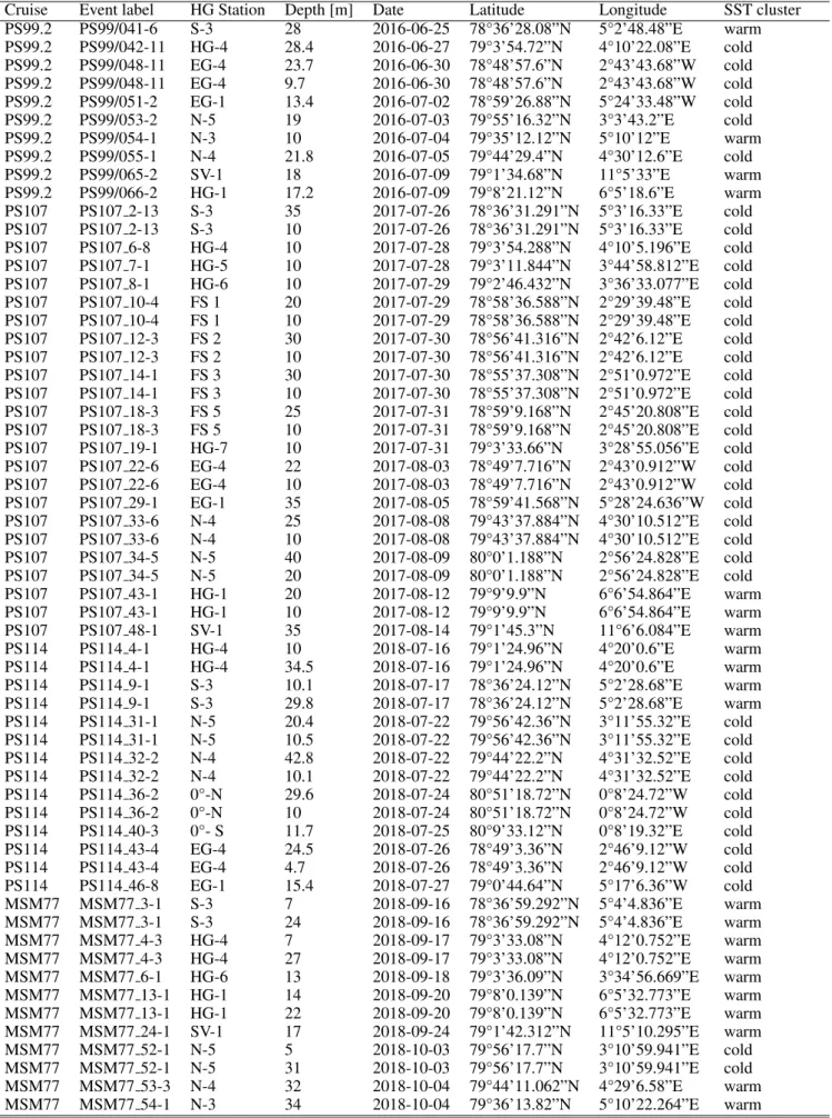
Table S1.Dates and locations of sample collections. SST cluster denotes whether a sample was classified as Atlantic (warm) or Polar (cold). PS99.1–PS114 were summer cruises, MSM77 was an autumn cruise. Event labels refer to the Pangaea database.

Cruise Event label HG Station Depth [m] Date Latitude Longitude SST cluster PS99.2 PS99/041-6 S-3 28 2016-06-25 78°36’28.08”N 5°2’48.48”E warm PS99.2 PS99/042-11 HG-4 28.4 2016-06-27 79°3’54.72”N 4°10’22.08”E cold PS99.2 PS99/048-11 EG-4 23.7 2016-06-30 78°48’57.6”N 2°43’43.68”W cold PS99.2 PS99/048-11 EG-4 9.7 2016-06-30 78°48’57.6”N 2°43’43.68”W cold PS99.2 PS99/051-2 EG-1 13.4 2016-07-02 78°59’26.88”N 5°24’33.48”W cold PS99.2 PS99/053-2 N-5 19 2016-07-03 79°55’16.32”N 3°3’43.2”E cold PS99.2 PS99/054-1 N-3 10 2016-07-04 79°35’12.12”N 5°10’12”E warm PS99.2 PS99/055-1 N-4 21.8 2016-07-05 79°44’29.4”N 4°30’12.6”E cold PS99.2 PS99/065-2 SV-1 18 2016-07-09 79°1’34.68”N 11°5’33”E warm PS99.2 PS99/066-2 HG-1 17.2 2016-07-09 79°8’21.12”N 6°5’18.6”E warm PS107 PS107 2-13 S-3 35 2017-07-26 78°36’31.291”N 5°3’16.33”E cold PS107 PS107 2-13 S-3 10 2017-07-26 78°36’31.291”N 5°3’16.33”E cold PS107 PS107 6-8 HG-4 10 2017-07-28 79°3’54.288”N 4°10’5.196”E cold PS107 PS107 7-1 HG-5 10 2017-07-28 79°3’11.844”N 3°44’58.812”E cold PS107 PS107 8-1 HG-6 10 2017-07-29 79°2’46.432”N 3°36’33.077”E cold PS107 PS107 10-4 FS 1 20 2017-07-29 78°58’36.588”N 2°29’39.48”E cold PS107 PS107 10-4 FS 1 10 2017-07-29 78°58’36.588”N 2°29’39.48”E cold PS107 PS107 12-3 FS 2 30 2017-07-30 78°56’41.316”N 2°42’6.12”E cold PS107 PS107 12-3 FS 2 10 2017-07-30 78°56’41.316”N 2°42’6.12”E cold PS107 PS107 14-1 FS 3 30 2017-07-30 78°55’37.308”N 2°51’0.972”E cold PS107 PS107 14-1 FS 3 10 2017-07-30 78°55’37.308”N 2°51’0.972”E cold PS107 PS107 18-3 FS 5 25 2017-07-31 78°59’9.168”N 2°45’20.808”E cold PS107 PS107 18-3 FS 5 10 2017-07-31 78°59’9.168”N 2°45’20.808”E cold PS107 PS107 19-1 HG-7 10 2017-07-31 79°3’33.66”N 3°28’55.056”E cold PS107 PS107 22-6 EG-4 22 2017-08-03 78°49’7.716”N 2°43’0.912”W cold PS107 PS107 22-6 EG-4 10 2017-08-03 78°49’7.716”N 2°43’0.912”W cold PS107 PS107 29-1 EG-1 35 2017-08-05 78°59’41.568”N 5°28’24.636”W cold PS107 PS107 33-6 N-4 25 2017-08-08 79°43’37.884”N 4°30’10.512”E cold PS107 PS107 33-6 N-4 10 2017-08-08 79°43’37.884”N 4°30’10.512”E cold PS107 PS107 34-5 N-5 40 2017-08-09 80°0’1.188”N 2°56’24.828”E cold PS107 PS107 34-5 N-5 20 2017-08-09 80°0’1.188”N 2°56’24.828”E cold PS107 PS107 43-1 HG-1 20 2017-08-12 79°9’9.9”N 6°6’54.864”E warm PS107 PS107 43-1 HG-1 10 2017-08-12 79°9’9.9”N 6°6’54.864”E warm PS107 PS107 48-1 SV-1 35 2017-08-14 79°1’45.3”N 11°6’6.084”E warm PS114 PS114 4-1 HG-4 10 2018-07-16 79°1’24.96”N 4°20’0.6”E warm PS114 PS114 4-1 HG-4 34.5 2018-07-16 79°1’24.96”N 4°20’0.6”E warm PS114 PS114 9-1 S-3 10.1 2018-07-17 78°36’24.12”N 5°2’28.68”E warm PS114 PS114 9-1 S-3 29.8 2018-07-17 78°36’24.12”N 5°2’28.68”E warm PS114 PS114 31-1 N-5 20.4 2018-07-22 79°56’42.36”N 3°11’55.32”E cold PS114 PS114 31-1 N-5 10.5 2018-07-22 79°56’42.36”N 3°11’55.32”E cold PS114 PS114 32-2 N-4 42.8 2018-07-22 79°44’22.2”N 4°31’32.52”E cold PS114 PS114 32-2 N-4 10.1 2018-07-22 79°44’22.2”N 4°31’32.52”E cold PS114 PS114 36-2 0°-N 29.6 2018-07-24 80°51’18.72”N 0°8’24.72”W cold PS114 PS114 36-2 0°-N 10 2018-07-24 80°51’18.72”N 0°8’24.72”W cold PS114 PS114 40-3 0°- S 11.7 2018-07-25 80°9’33.12”N 0°8’19.32”E cold PS114 PS114 43-4 EG-4 24.5 2018-07-26 78°49’3.36”N 2°46’9.12”W cold PS114 PS114 43-4 EG-4 4.7 2018-07-26 78°49’3.36”N 2°46’9.12”W cold PS114 PS114 46-8 EG-1 15.4 2018-07-27 79°0’44.64”N 5°17’6.36”W cold MSM77 MSM77 3-1 S-3 7 2018-09-16 78°36’59.292”N 5°4’4.836”E warm MSM77 MSM77 3-1 S-3 24 2018-09-16 78°36’59.292”N 5°4’4.836”E warm MSM77 MSM77 4-3 HG-4 7 2018-09-17 79°3’33.08”N 4°12’0.752”E warm MSM77 MSM77 4-3 HG-4 27 2018-09-17 79°3’33.08”N 4°12’0.752”E warm MSM77 MSM77 6-1 HG-6 13 2018-09-18 79°3’36.09”N 3°34’56.669”E warm MSM77 MSM77 13-1 HG-1 14 2018-09-20 79°8’0.139”N 6°5’32.773”E warm MSM77 MSM77 13-1 HG-1 22 2018-09-20 79°8’0.139”N 6°5’32.773”E warm MSM77 MSM77 24-1 SV-1 17 2018-09-24 79°1’42.312”N 11°5’10.295”E warm MSM77 MSM77 52-1 N-5 5 2018-10-03 79°56’17.7”N 3°10’59.941”E cold MSM77 MSM77 52-1 N-5 31 2018-10-03 79°56’17.7”N 3°10’59.941”E cold MSM77 MSM77 53-3 N-4 32 2018-10-04 79°44’11.062”N 4°29’6.58”E warm MSM77 MSM77 54-1 N-3 34 2018-10-04 79°36’13.82”N 5°10’22.264”E warm