Colorimetric detection of selected gases for work and food safety applications
DISSERTATION ZUR ERLANGUNG DES DOKTORGRADES DER NATURWISSENSCHAFTEN (DR. RER. NAT.) DER FAKULTÄT CHEMIE UND PHARMAZIE DER UNIVERSITÄT REGENSBURG
vorgelegt von
Julia Linhardt
Diese Doktorarbeit entstand in der Zeit von Januar 2013 bis Dezember 2015 an der Fraunhofer-Einrichtung für Mikrosysteme und Festkörper-Technologien (EMFT) in Kooperation mit dem Institut für Analytische Chemie, Chemo-und Biosensorik an der Universität Regensburg.
Die Arbeit wurde durchgeführt bei Prof. Dr. Joachim Wegner.
Promotionsgesuch eingereicht: 29. Januar 2016 Kolloquiumstermin: 18. März 2016 Prüfungsausschuss:
Vorsitzender: Prof. Dr. Oliver Tepner Erstgutachter: Prof. Dr. Joachim Wegener
To Roland & my family
Table of contents
A Introduction ... 1
B Theoretical background ... 9
1 Sensors in digital cameras ... 9
2 Multivariate analysis – Principal Component Analysis ... 12
3 Color spaces ... 17
4 References ... 21
C Detection of volatile aldehydes for food safety applications ... 23
1 Introduction ... 23
1.1 Autoxidation of fatty acids ... 25
1.2 Measuring the autoxidation state of fatty food ... 31
1.3 Hexanal as indicator substance for rancidity of fats and oils ... 37
1.4 Measuring methods for hexanal ... 40
1.5 Intelligent food packaging ... 42
1.6 Reaction mechanism of Schiff’s reagent with aldehydes ... 45
2 Objective ... 47
3 Materials and Methods ... 48
3.1 Preparation of indicator particles ... 48
3.2 Preparation of measurement samples by applying PTFE as barrier ... 48
3.3 Preparation of measurement samples by immobilizing indicator particles in a polyvinyl acetate matrix... 50
3.4 Measurement setup ... 51
3.5 Data processing ... 53
3.6 Adjustment of aldehyde concentrations ... 54
3.7 General procedure for data evaluation... 56
4 Results and Discussion ... 61
4.1 Determination of best composition for Schiff’s reagent@silica ... 61
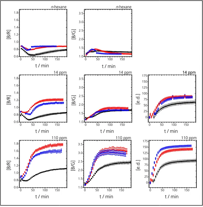
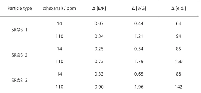
4.2 Calibration measurements ... 63
4.3 Comparison of limits of detection (LOD) and sensitivities ... 84
4.4 Assessment of cross sensitivities ... 87
4.5 Investigating long-term stability of indicator particles ... 90
4.6 Immobilization of particles in a polyvinyl acetate matrix ... 92
4.7 Application to real food samples ... 96
5 Summary and conclusion ... 102
6 References ... 103
D Detection of carbon monoxide for work safety applications ... 109
1 Introduction ... 109
2 Objective ... 115
3 Materials and Methods ... 116
3.1 Synthesis of indicator dyes ... 117
3.2 Sensor fabrication ... 119
3.3 Experimental setup for reflection measurements ... 120
3.4 Experimental setup for absorbance measurements ... 122
3.5 Determination of absorption coefficients ... 123
3.6 Determination of limits of detection (LOD) and sensitivity ... 124
3.7 Data evaluation... 124
4 Results and Discussion ... 126
4.1 Photophysical properties of indicator dyes ... 126
4.2 Choice of matrix polymers ... 129
4.3 Calibration by reflection measurements (0 – 10% CO) ... 132
4.4 Calibration by absorbance measurements (0 – 100 ppm CO) ... 135
4.5 Assessment of cross sensitivities ... 138
5 Summary and conclusion ... 140
6 References ... 141
E Detection of ammonia for work safety applications ... 145
1 Introduction ... 145
1.1 Sources of ammonia and application fields for ammonia sensors ... 145
1.2 Ammonia sensing principles ... 147
1.3 Sensor systems in textiles ... 149
2 Objective ... 155
3 Materials and Methods ... 156
3.1 Dyeing with ammonia-sensitive probes ... 156
3.2 Preparation of measurement samples ... 157
3.3 Measurement setup and data processing ... 157
3.4 Adjustment of amine concentrations ... 158
3.5 General procedure for data evaluation... 159
3.5.1 Color change evaluation of bromothymol blue dyed polyamide fabric (BTB-PA) ... 160
3.5.2 Color change evaluation of cresol red dyed polyamide fabric (CR-PA)... 161
3.5.3 Color change evaluation of methyl red dyed polyamide fabric (CR-PA) ... 162
3.5.4 Determination of limits of detection (LOD) and sensitivities... 163
3.5.5 Determination of response and reverse times ... 163
4 Results and Discussion ... 165
4.1 Calibration measurements with ammonia ... 165
4.1.1 Bromothymol blue dyed polyamide (BTB-PA) ... 165
4.1.2 Cresol red dyed polyamide (CR-PA) ... 169
4.1.3 Methyl red dyed polyamide (MR-PA) ... 173
4.2 Limits of detection (LOD), sensitivity, and response times ... 176
4.3 Response and reverse behavior of sensor fabrics ... 177
4.3.1 Bromothymol blue dyed polyamide ... 178
4.3.2 Cresol red dyed polyamide ... 179
4.3.3 Methyl red dyed polyamide... 180
4.3.4 Response and reverse times ... 180
4.4 Assessment of cross sensitivities to acids ... 182
4.4.1 Bromothymol blue dyed polyamide ... 183
4.4.2 Cresol red dyed polyamide ... 185
4.4.3 Methyl red dyed polyamide... 187
4.5 Response of sensor textiles to various amines ... 190
4.5.1 Bromothymol blue dyed polyamide ... 191
4.5.2 Cresol red dyed polyamide ... 193
4.5.3 Methyl red dyed polyamide... 195
4.5.4 Comparison of sensor responses to various amines ... 197
4.6 Calibration of bromothymol blue dyed polyamide fabric with ethylamine, diethylamine, and triethylamine ... 199
4.7 Long-term stability of sensor textiles ... 201
5 Summary and conclusion ... 203
F Summary ... 207
1 Summary in English ... 207
2 Summary in German ... 209
G Appendix ... 211
1 Abbreviations and symbols ... 211
2 Regents and materials ... 215
3 Instrumentation and consumable ... 216
4 Software ... 216
5 Supplementary figures and tables ... 217
H Curriculum vitae ... 247
I Acknowledgements ... 251
J Declaration ... 253
A Introduction
Detection of gases is feasible by transforming physical or chemical sensor information to electrical signals via various different methods. Physical information is provided e.g. by molecular mass, diffusion properties or the molecular structure of a gas. Chemical information in contrast includes reactivity like oxidizability or reducibility of the corresponding gas.
A general description of chemical sensors is provided by the Cambridge definition: “Chemical sensors are miniaturized devices that can deliver real time and on-line information on the presence of specific compounds or ions in even complex samples”. 1
Figure A1 depicts the schematic setup of a chemical sensor including the analyte to be measured and a suitable sensor platform with a transducer unit. The obtained chemical information is converted into an electrical signal which correlates with the analyte concentration.
As a result the present amount of analyte can be derived from the raw data via suitable signal processing methods and communicated e.g. by a visual display or an acoustic sound upon exceeding a certain threshold signal.
Figure A1. Schematic sequence of a chemical sensor setup according to Cambridge definition. 1
Signal transduction can be performed via different principles. One possibility is provided by resistive methods which generally make use of conductive sensor films that change their resistance depending on the present analyte concentration. 2 Capacitive sensors in contrast detect the presence of gaseous analytes by induced alterations of a sensitive dielectric. 3–5 Potentiometric methods instead quantify the potential difference between a measuring and a reference electrode. This difference originates from the interaction of gaseous analytes with the measuring electrode while any contact to the reference electrode is avoided. 6–8 Another measuring principle
Analyte
Sensor platform/
Transduction Signal processing
Analyte concentration
Additionally, gravimetric methods can be applied for signal transduction. Gravimetric sensors utilize a mass change induced by adsorbed gas molecules, for example on piezoelectric crystals which as a result exhibit modified resonance frequencies. 12 The optoelectronic measuring principle finally provides an example which is especially important for optical chemical sensors. 13–
15 For this kind of sensors, optical information is transduced into electrical signals by applying visible, infrared or UV light. 16,17
After signal transduction by any of the above mentioned transducer methods signal processing is performed by mathematical and statistical approaches. Thus, the electric signal is transformed to e.g. a concentration which is communicated via display.
Optical chemical sensors have been a steadily growing research area with a number of successful applications during the last decade. Advantages of optical chemical sensors are for example their low manufacturing costs and easy miniaturization. Moreover, they enable non- invasive measurements, remote and online sensing and often provide unmatched sensitivity.
Furthermore, they are often non-toxic in use, easy to handle, and can be applied in hazardous environments or point-of-care diagnostics, respectively. 18,19
Optical chemical sensors are mostly based on fluorescence measurements and monitor lifetime, polarization, intensity, and quenching or energy transfer processes (FRET). 20–24 UV/Vis absorption provides an alternative detection method for optical chemical systems. 15,25–28 In general, these sensors can be separated in two different categories: direct (label-free) sensors and reagent- mediated (label-based) sensing systems. 1
Direct optical sensors detect the gaseous analyte by its intrinsic optical properties such as absorption or fluorescence. The absorption of IR light for example reports on the vibrational modes of a specific gas molecule and can be measured via an absorption cell which contains the corresponding analyte gas. This principle is applicable for various gases like CO2, CO, NO2, NH3, and CH4. 1,29,30
In reagent-mediated systems an intermediate agent is used to monitor analyte concentrations, e.g. an analyte sensitive dye molecule. An optical response of the applied reagent can be detected upon either reversible or irreversible reaction with analyte molecules. 31–35 Reagent-mediated techniques are useful for analytes which do not provide sufficiently appropriate intrinsic, optical properties. A well known example for this principle is oxygen sensing which detect a change in luminescence intensity and/or lifetime of a reagent in the presence of oxygen. 36–39
The indirect measuring principle requires an immobilized reagent to facilitate interaction with gaseous molecules. In recent years this was usually performed by applying solid phase
immobilization by covalent or ionic binding, or encapsulation of the reagent dye. 22,40–42 A wide range of sensor configurations and applications is feasible especially with immobilization matrices that can be conveniently coated onto various substrates (e.g. sol-gel glasses or polymer coatings).
43 Figure A2 shows the setup of sensors consisting of a reagent immobilized in a suitable matrix and coated on a solid support. After reacting with a present analyte the sensor dye changes its structural and optical properties.
Figure A2. Principle of sensors consisting of reagents immobilized in e.g. polymer matrices. The optical properties of the dye are modified after reaction with an analyte.
Structural characteristics of matrix materials strongly influence reagent immobilization, stability, and permeability to the analyte. 41 Herein only polymer materials will be discussed, which generally have a distinct effect on the sensor performance. Response time and selectivity, for instance, are greatly dependent on the diffusion properties of the respective analyte through the matrix material. 14,37 Furthermore, the thickness of polymer films is generally a compromise between sensitivity and response time of the sensing system. While thicker films provide higher sensitivity, the response time of the sensor increases. Additionally, the polymer material acts as a support for the active chemical reagent (sensor dye) and can provide a protective covering.
Furthermore, a certain degree of analyte selectivity can be achieved which is attributed to the structural features of the polymer material. 43 Possible polymeric supports include polyester, polyamide, or similar polymers used in textile fabrication.
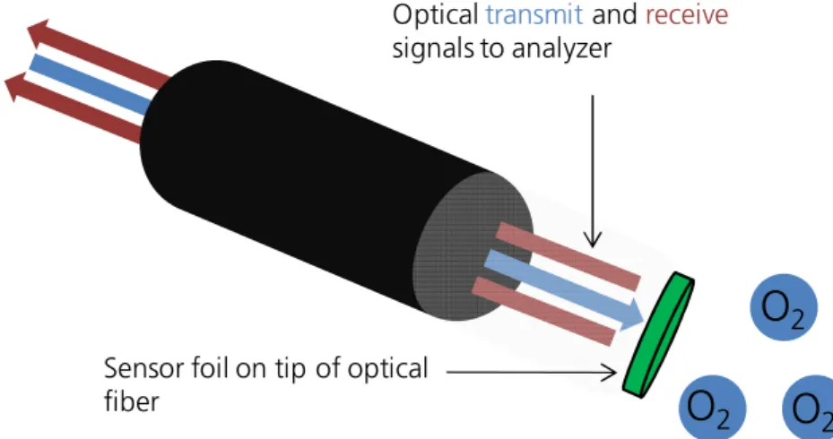
Optical chemical sensors have already been developed for gaseous analytes such as O2, SO2, SH2, and CO2. 22,24,37,43–47 An example of a commercially available oxygen sensor, manufactured by PreSens Precision Sensing (Regensburg, Germany) sketched in Figure A3. The sensor combines several techniques which were previously explained. The oxygen sensing spots consist of a
matrix polymer
solid support
analyte sensor dye
sensor dye after reacting with analyte
concentration. Figure A3 shows this optical measuring principle and the sensor foil fixed on the fiber’s tip. In the presence of oxygen the optical properties of the sensor foil is changed which can be detected by a modified signal transported via the fiber. 48 Even non-invasive oxygen sensing is possible using these sensor spots by simply applying them inside glass bottles containing any liquid samples. Thus, detection of both, dissolved and gaseous oxygen is feasible from the outside of a vessel by simply monitoring the partial pressure. 49
Figure A3. Optical measuring principle of oxygen sensing by PreSens Precision Sensing, Regensburg. 48
Many of the early chemical sensor techniques were based on colorimetric methods, i.e. applying a color change of colorimetric sensor dyes in the presence of particular analytes. 19 A big advantage of colorimetric sensors is their visibility by the naked eye which allows a qualitative evaluation even without power consuming electronic devices. By combining them with compact, portable photometers, conversion of the analyte concentration into an electrical signal is also possible, and thus, the generation of a sensor according to the Cambridge definition. 1,18 The probably best-known colorimetric sensor dyes are pH-dependent dyes like bromothymol blue, cresol red, or methyl red. 16,50–52
Irreversible colorimetric indicators, however, are not considered as sensors according to the Cambridge definition, as they do not show a reversible response and thus do not allow real-time monitoring of analyte concentration. As a result these irreversible indicators can only be used as single-shot probes and are restricted to applications which do not require a continuous detection of analytes. 18
In the present thesis irreversible, colorimetric indicator dyes were applied e.g. for the detection of decomposition products of fat-containing foods. The indicators were directly incorporated into food packaging for detecting gaseous analytes generated by oxidation processes. For this purpose
O
2O
2O
2Optical transmitandreceive signals to analyzer
Sensor foil on tip of optical fiber
an irreversible color change is advantageous to avoid false-negative results caused by leakage of volatile analytes from opened or resealed (e.g. for oil bottles) food packages.
Although colorimetric changes of either reversible or irreversible colorimetric indicator dyes can be detected by the naked eye, it can still be difficult to quantify the analyte concentration. For this purpose suitable video cameras, digital color analyzers, scanners or custom portable readers have already been employed. 53–56
Figure A4. A: Bayer color filter; B: CMOS sensor; 57 C: Schematic of the additive RGB color space. 58
In the present thesis digital color cameras were applied to quantify the color change of amine sensors for work safety applications and aldehyde indicators for food safety applications. In digital color cameras color filters (e.g. Bayer filter, see Figure A4, A) in combination with CCD- or CMOS camera sensors (Figure A4, B) are integrated for the generation of electrical signals. 59,60 The working principle of those image sensors is explained in detail in part B (chapter 1). Digital color cameras generally use the RGB color space (Figure A4, C) for image recording since the color filter consists of red, green, and blue single filters. Besides the RGB color space various other color spaces exist 51,53 which is intensely discussed in part B (chapter 2).
A B C
References
(1) McDonagh, C.; Burke, C. S.; MacCraith, B. D. Chem. Rev. 2008, 108 (2), 400–422.
(2) Chabukswar, V.; Pethkar, S.; Athawale, A. A. Sens. Actuators, B 2001, 77 (3), 657–663.
(3) Dai, C.-L.; Lu, P.-W.; Chang, C.; Liu, C.-Y. Sensors 2009, 9 (12), 10158–10170.
(4) Gu, L.; Huang, Q.-A.; Qin, M. Sens. Actuators, B 2004, 99 (2-3), 491–498.
(5) Matsuguchi, M. J. Electrochem. Soc. 1991, 138 (6), 1862.
(6) Liang, R.-N.; Song, D.-A.; Zhang, R.-M.; Qin, W. Angew. Chem. 2010, 122 (14), 2610–2613.
(7) Liang, R.; Zhang, R.; Qin, W. Sens. Actuators, B 2009, 141 (2), 544–550.
(8) Prasad, K.; Prathish, K. P.; Gladis, J. M.; Naidu, G.; Rao, T. P. Sens. Actuators, B 2007, 123 (1), 65–70.
(9) Wang G.-F., Li M.-G., Gao Y.-C., Fang B. Sensors 2004, 4 (9), 147–155.
(10) Saleh Ahammad, A. J.; Lee, J.-J.; Rahman, M. A. Sensors 2009, 9 (4), 2289–2319.
(11) Lawrence, N. S.; Davis, J.; Jiang, L.; Jones, Tim G. J.; Davies, S. N.; Compton, R. G.
Electroanalysis 2000, 12 (18), 1453–1460.
(12) Pandey, S. K.; Kim, K.-H.; Tang, K.-T. TrAC, Trends Anal. Chem. 2012, 32, 87–99.
(13) Hyakutake, T.; Taguchi, H.; Kato, J.; Nishide, H.; Watanabe, M. Macromol. Chem. Phys. 2009, 210 (15), 1230–1234.
(14) Schäferling, M. Angew. Chem. Int. Ed. Engl. 2012, 51 (15), 3532–3554.
(15) Alves, F. L.; Raimundo, I. M.; Gimenez, I. F.; Alves, O. L. Sens. Actuators, B 2005, 107 (1), 47–
52.
(16) Nakamura, N.; Amao, Y. Sens. Actuators, B 2003, 92 (1-2), 98–101.
(17) Janata J.; Josowicz M.; Vanysek P.; DeVaney D.M. Anal. Chem. 1998, 70 (12), 179R-208R.
(18) Stich, M. I. J.; Fischer, L. H.; Wolfbeis, O. S. Chem. Soc. Rev. 2010, 39 (8), 3102–3114.
(19) Newman, J.; Bogue, R. Sens. Rev. 2007, 27 (2), 86–90.
(20) Hradil, J.; Davis, C.; Mongey, K.; McDonagh, C.; MacCraith, B. D. Meas. Sci. Technol. 2002, 13 (10), 1552–1557.
(21) Borisov, S. M.; Wolfbeis, O. S. Anal. Chem. 2006, 78 (14), 5094–5101.
(22) Stich, M. I. J.; Nagl, S.; Wolfbeis, O. S.; Henne, U.; Schaeferling, M. Adv. Funct. Mater. 2008, 18 (9), 1399–1406.
(23) He, C.-L.; Ren, F.-L.; Zhang, X.-B.; Han, Z.-X. Talanta 2006, 70 (2), 364–369.
(24) Razek, T. Talanta 1999, 50 (3), 491–498.
(25) McDonagh, C.; Kolle, C.; McEvoy, A. K.; Dowling, D. L.; Cafolla, A. A.; Cullen, S. J.; MacCraith, B. D. Sens. Actuators, B 2001, 74 (1–3), 124–130.
(26) Ali, R.; Lang, T.; Saleh, S. M.; Meier, R. J.; Wolfbeis, O. S. Anal. Chem. 2011, 83 (8), 2846–
2851.
(27) Nakamura, N.; Amao, Y. Anal. Bioanal. Chem. 2003, 376 (5), 642–646.
(28) Zhang, C.; Bailey, D. P.; Suslick, K. S. J. Agric. Food Chem. 2006, 54 (14), 4925–4931.
(29) Timmer, B.; Olthuis, W.; van Berg, A. d. Sens. Actuators, B 2005, 107 (2), 666–677.
(30) Sazhin, S. G.; Soborover, E. I.; Tokarev, S. V. Russ. J. Nondestr. Test. 2003, 39 (10), 791–806.
(31) Kim, H. N.; Guo, Z.; Zhu, W.; Yoon, J.; Tian, H. Chem. Soc. Rev. 2011, 40 (1), 79–93.
(32) Kim, H. N.; Ren, W. X.; Kim, J. S.; Yoon, J. Chem. Soc. Rev. 2012, 41 (8), 3210–3244.
(33) Vo, E.; Zhuang, Z. Arch. Environ. Contam. Toxicol. 2009, 57 (1), 185–192.
(34) Abel, T.; Ungerböck, B.; Klimant, I.; Mayr, T. Chem. Cent. J. 2012, 6 (1), 124.
(35) Lobnik, A.; Wolfbeis, O. S. Sens. Actuators, B 1998, 51 (1-3), 203–207.
(36) Quaranta, M.; Borisov, S. M.; Klimant, I. Bioanal. Rev. 2012, 4 (2-4), 115–157.
(37) Amao, Y. Microchim. Acta 2003, 143 (1), 1–12.
(38) Borisov, S. M.; Klimant, I. Anal. Chem. 2007, 79 (19), 7501–7509.
(39) Fercher, A.; Borisov, S. M.; Zhdanov, A. V.; Klimant, I.; Papkovsky, D. B. ACS Nano 2011, 5 (7), 5499–5508.
(40) Barbe, J.-M.; Canard, G.; Brandès, S.; Guilard, R. Chem. Eur. J. 2007, 13 (7), 2118–2129.
(41) Harsányi, G. Sens. Rev. 2000, 20 (2), 98–105.
(42) Dickert, F. L. Adv. Mater. 1997, 9 (9), 762.
(43) Brook, T. E.; Narayanaswamy, R. Sens. Actuators, B 1998, 51 (1-3), 77–83.
(44) Borisov, S. M.; Waldhier, M. C.; Klimant, I.; Wolfbeis, O. S. Chem. Mater. 2007, 19 (25), 6187–
6194.
(45) Hodgkinson, J.; Tatam, R. P. Meas. Sci. Technol. 2013, 24 (1), 1–59.
(46) Aydogdu, S.; Ertekin, K.; Suslu, A.; Ozdemir, M.; Celik, E.; Cocen, U. J. Fluoresc. 2011, 21 (2), 607–613.
(47) Chen, B.; Li, W.; Lv, C.; Zhao, M.; Jin, H.; Jin, H.; Du, J.; Zhang, L.; Tang, X. Analyst 2013, 138 (3), 946–951.
(48) PreSens Precision Sensing. Oxygen Probes. 2015 [cited: 2015 october 11]; available from:
http://www.presens.de/products/brochures/category/sensor-probes/brochure/oxygen-probes.html.
(49) PreSens Precision Sensing. Non-Invasive Optical Oxygen Sensors. 2015 [cited: 2015 october 11]; available from: http://www.presens.de/products/brochures/category/sensor- probes/brochure/non-invasive-oxygen-sensors.html.
(50) McMurray, H. N. J. Mater. Chem. 1992, 2 (4), 401.
(51) Shen, L.; Hagen, J. A.; Papautsky, I. Lab Chip 2012, 12 (21), 4240–4243.
(52) Rodríguez, A. J.; Zamarreño, C. R.; Matías, I. R.; Arregui, F. J.; Cruz, R. F. D.; May-Arrioja, D. A.
(54) Feng, L.; Musto, C. J.; Suslick, K. S. J. Am. Chem. Soc. 2010, 132 (12), 4046–4047.
(55) Meier, R. J.; Schreml, S.; Wang, X.-d.; Landthaler, M.; Babilas, P.; Wolfbeis, O. S. Angew. Chem.
Int. Ed. 2011, 50 (46), 10893–10896.
(56) Sen, A.; Albarella, J.; Carey, J.; Kim, P.; McNamara III, W. B. Sens. Actuators, B 2008, 134 (1), 234–237.
(57) Moore M. How does a DSLR work? 2012 [cited: 2015 october 11]; available from:
https://martinmoorephotography.wordpress.com/2012/04/04/how-does-a-dslr-work/.
(58) Corel Center. Additive Farbmischung. 2015 [cited: 2015 october 11]; available from:
http://www.corelcenter.de/knowledgebase/farbmodelle.html.
(59) Marczewska, B. Radiat. Prot. Dosim. 2006, 120 (1-4), 129–132.
(60) Stich, M. I. J.; Borisov, S. M.; Henne, U.; Schäferling, M. Sens. Actuators, B 2009, 139 (1), 204–
207.
B Theoretical background 1 Sensors in digital cameras
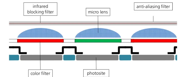
The color change of indicators used in this thesis is quantified by a digital color camera. Photos are taken during the reaction with diverse analytes and evaluated by splitting into the red, green, and blue color channels. In digital single lens reflex cameras (DSLR-cameras) the most commonly used sensor is the so-called CMOS (Complementary Metal-Oxide Semiconductor) sensor. Another one is CCD (Charge Coupled Device) sensor which is less often used. The difference of both sensors is simply the control and readout of the individual photosites. Figure B1 shows the schematic set-up of an image sensor as well as the working principle which are nearly identical for both sensors. 1
Figure B1. Schematic set-up of an image sensor integrated in digital color cameras. 2
An object is projected onto the surface of the sensor when the camera is taking a picture. The sensor consists of numerous photosites (or photodiodes) collecting photons as long as the shutter speed allows to. 3 The more photons are collected by the individual photosite, the higher is the brightness of the related pixel in the picture. The light collection is supported by micro lenses which are arranged on top of each photosite and bundle the incoming light in the light-sensitive areas. Before the light is collected by these micro lenses it first has to pass two filters. The anti- aliasing filter smooths the incoming light to prevent the Moiré effect. The infrared blocking filter avoids infrared contamination of the sensor which would lead to off-color of the received
photosite color filter
micro lens
anti-aliasing filter infrared
blocking filter
In their native state image sensors are color blind and can only detect brightness values. 4,5 To enable color capture, color filters are placed between each photosite and the related micro lens.
These color filters are arranged as array above the photosites and are red, green or blue colored.
The most commonly applied color patterns derive in some way from the Bayer pattern. 6 Here, red, green, and blue pixels are arranged next to each other in a plain. Thus, each photosite becomes sensitive for one of the primary colors (Figure B2). 2–5
Figure B2. Typical Bayer pattern applied in color filter arrays. Red, green, and blue filters alternate in plain.
The human eye is most sensitive to green light, thus, twice as much green filters are arranged in the Bayer pattern as red and blue ones. 5 Since each photosite is only sensitive for one color, the signal processor in the camera needs to calculate the other colors. Via interpolation the missing colors are calculated based on the information received from surrounding pixels. 2,5 This process is also called color reconstruction or demosaicing and generates three different color channels for each pixel.
All digital pixels (picture-elements) have the same size and form. The only difference is their brightness and coloring. Since the photosites in image sensors are arranged in columns and rows, the pixels in digital pictures also have this layout. The pixel number of a photo depends on the number of photosites in the sensor of the camera. 2,4 Thus, the number of pixels can vary from 4288 x 2848 in amateur cameras to 7360 x 4912 (wide x height) pixels in a professional camera.
An increasing density of photosites results in higher resolution of the generated picture. 4
In digital cameras the image quality can be influenced by diverse camera settings. These are the ISO value, shutter speed (exposure time), and aperture size which are described in more detail below.
Sensor sensitivity (ISO value)
Increasing the sensor sensitivity implies an intensification of the electrical signal which one photon produces when hitting a photosite. This becomes important at poor lighting conditions. However, an increase of the camera’s gain can result into a high noise. 7 The adjusted sensitivity of the sensor is specified in ISO values, e.g. with ISO 800 the sensor is twice as sensitive as with ISO 400.
2
Shutter speed
The shutter regulates the time that the sensor captures incoming light (exposure time). The shutter can operate either mechanically or electrically by activating the sensor for a certain period of time. Professional DLSR cameras often hold both types whereby the mechanical one is used for longer and the electrical ones for shorter shutter speeds. 2,8 However, when setting the exposure time too high, motion blur can be caused by scene motion or slightly moving the camera. 7
F-Stop
The f-Stop describes the aperture size. When opening the aperture more photons can pass in the same time as it is the case for a smaller one. Consequently, opening the aperture causes an increased brightness of the received image. The f-stops are specified in values like f/2, f/4, or f/16 with two times more light passing the aperture at f/2 than f/4. 8 However, opening the aperture can cause a reduction in the depth of field and the aperture is highly limited by the type of lens. 7
White Balance
White balance means the adjustment of digital cameras to different color temperatures of surrounding light. Light consists of electromagnetic radiation which includes a broad wavelength range. While in the morning ambient light includes more of the blue part, light in the evening includes more of the red part of the electromagnetic spectrum. Moreover, artificial light often consists of a very high amount of blue light. Hence, for avoiding color fault in digital images, a white balance has to be performed either by the automatic white balance function of the camera or by doing manual white balance.
2 Multivariate analysis - Principal Component Analysis
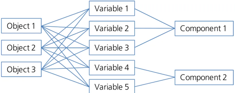
The Principal Component Analysis (PCA) is a method of multivariate analysis for the reduction of complex raw data. PCA is a descriptive-exploratory technique and identifies structures or relationships in large sets of variables. It separates highly correlated variables from less correlated ones which are summarized in groups, named as components. The general principle of PCA is shown in Figure B3. In this example three different objects are characterized regarding five different variables. PCA identifies a high correlation between variables 1-3 and between variables 4 and 5. Hence, these groups of variables are summarized to components 1 and 2. 9,10
Additionally, the correlation of variables to components can also be shown quantitatively by calculating so-called component-values. These component-values for each variable can then be used instead of the original data and represented graphically. 9
Figure B3. Schematic representation of principle component analysis (PCA). Correlated variables determined for diverse objects are summarized to components.
Before determining these component-values a statistical analysis needs to be applied for quantifying relations between individual variables. This relation is described by correlation coefficients easily summarized in correlation matrices. Afterwards, the number of extracted components is set by the user. Here, a compromise between data reduction and information loss needs to be found.
In general, the process of principal component analysis can be divided into four steps. These are the determination of correlation matrix, extraction of components, and the assignment of component numbers and component-values. These five steps are described more precisely in the below. 9
Variable 1 Variable 2 Variable 3 Variable 4 Variable 5
Component 1
Component 2 Object 1
Object 2 Object 3
Determining the correlation matrix
Correlations between variables have to be quantified by calculating the so-called correlation coefficients. Equation B1 shows the determination of the correlation coefficient r between two variables x1 and x2. 9,10
2 2 k2 2 1 K
1
k k1
2 k2 K
1
k k1 1
x2 x1,
) x x ( ) x (x
) x (x ) x (x r
−
⋅
−
−
⋅
−
=
∑
∑
=
= Eq. B1
xk1 and xk2 value of variable 1 and variable 2 of object k x1and x2 means of variable 1 and 2 over all objects
x2
rx1, correlation coefficient of variable 1 and variable 2
By calculating all correlation coefficients for the five variables (Figure B3) a correlation matrix is generated. A typical correlation matrix for five different variables is depicted in Table B1.
Table B1. Typical correlation matrix for five different variables.
Before calculating the correlation matrix, the raw data is often standardized. This means, calculating the difference between the mean of a variable and the individual variable values of a specific object k. The result is then divided by the standard deviation generated by forming the mean value (Equation B2).
Variable 1 Variable 2 Variable 3 Variable 4 Variable 5 Variable 1 1.0
Variable 2 0.3 1.0
Variable 3 0.3 0.7 1.0
Variable 4 0.04 0.9 0.2 1.0
Variable 5 0.1 0.2 0.7 0.2 1.0
j kj j
kj s
x
z x −
= Eq. B2
z kj standardized value of variable j of object k x kj value of variable j for object k
xj mean of variable j over all objects
s j standard deviation of the mean of variable j over all objects
After the correlation matrix has been established the matrix and thus, also the original data is suitable for principal component analysis. For this proof, there are some statistical methods available such as testing significance of the correlations, the inverse of the correlation matrix, the Bartlett-test (test of sphericity), the anti-image-covariance-matrix, and the Kaiser-Meyer-Olkin- criterion. However, these statistical methods are not further explained in this context. The software used in this thesis for PCA applies one of these methods automatically, or the user can select one based on his/her own preferences. 9,10
Extraction of components
By applying the fundamental theorem of PCA components can be calculated based on the correlation matrix. The basic assumption is that each original variable xj (or its standardized variable zj)can be described by a linear combination of different (hypothetic) components. The mathematical relationship is shown by Equation B3. 9
k0 j0 k2
j2 k1 j1
kj a p a p ... a p
x = ⋅ + ⋅ + + ⋅ Eq. B3
In Equation B3 parameters p represent the components and parameters a the loadings of the components. Thereby, the loadings describe the relationship between a component and the variables. This relationship is named the correlation coefficients between components and variables. 9
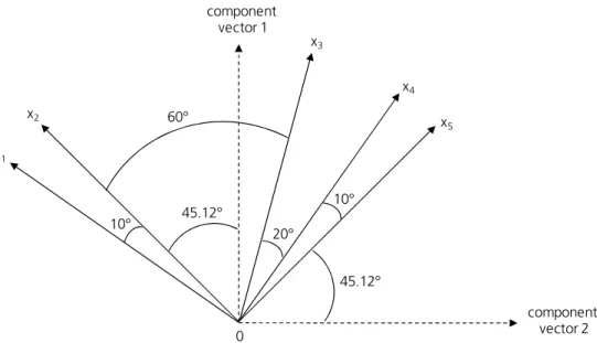
The correlation matrix can also be represented by a vector diagram (Figure B4). Each vector represents a variable (x1-x5) and the cosine of the angle between two vectors is a measure for the correlation coefficient of these two variables. The more variables are included, the more dimensions are necessary for positioning all vectors. The aim of PCA is representing all correlation coefficients in the smallest possible dimension. Thereby, the number of necessary axes reflects the number of components. 9
Figure B4. Vector diagram of five variables x1-x5 and resultant component vectors 1 and 2. Angles between the vectors represent the respective correlation coefficients.
In Figure B4 the resultante of all five vectors describes the first component. The second component which has to be independent from the first component is represented by the vector starting in the origin and being orthogonal to the vector of component 1.
Afterwards, the correlation of the variables to extracted components must be quantified. This correlation is reflected by component loadings. Those can be read out from the respective vector diagram as well since the angles between the vector of a variable and the component vector represent the respective component loading. E.g. in Figure B4, the component loading of variable x2 to component 1 is the cosine of 45.12°.
Number of components
There is no unique regulation for determining the number of components, thus, the amount is regulated at the discretion of the user. However, some statistical methods can simplify the decision. The most frequently used methods are the Kaiser-Criterion and the Scree-Test whereby both procedures are very similar in its mathematical operations.
First of all, the Eigenvalues need to be calculated. The Eigenvalue of a component is the sum of the square component loadings of one component over all variables. The Kaiser-Criterion indicates that the number of components to be extracted is the same as the number of Eigenvalues with a value higher than 1. In Scree-tests all Eigenvalues are plotted in a coordinate
60°
45.12°
45.12°
10°
10°
20°
x1 x2
x3
x4 x5 component
vector 1
component vector 2 0
Determination of component values
Component values need to be determined in order to quantify the correlation of objects to extracted components. The component values are calculated by complex matrix transformations which are not explained within the scope of this thesis.
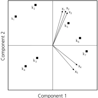
The determined values can be represented graphically via a PCA bi-plot. In Figure B5 component values for two components of seven objects x1-x7 are plotted as well as the vector loadings of the original variables x1-x5. 9
Figure B5. Typical PCA bi-plot showing the component values for two components of objects k and the variable vectors x.
k1
k2
k4 k3
k5
k6
k7
x5
x4 x3 x2 x1
Component 1
Component2
3 Color spaces
A color space is a scientific way to organize colors in a three-dimensional representation. The human visual system (HVS) is able to sense a part of the electromagnetic spectrum between wavelengths of 300 and 830 nm. The HVS cannot detect all possible parts of the visible spectrum, however, is able to group various wavelength into colors. Via defined color spaces it is possible to describe different colors as perceived and processed by people, machines, and programs. 11,12
A color itself is just the brains reaction to a specific stimulus. Although we can precisely describe colors by measuring its wavelength, recognizing colors by human eyes leads to redundancies since the eye is just sensitive to brightness and the three colors red, green, and blue. Thus, diverse color spaces were developed for specifying, visualizing, and describing color information. 12 In general, these can be categorized into three different groups. 11,13 The first group is formed by the color spaces based on the properties of the HVS. These are the RGB color spaces and spaces based on the opponent color theory. The second group are application specific color spaces adopted from television (TV) systems (YUV and YIQ color space), photo systems (Kodak PhotoYCC color space) and printing systems (CYMK color space). The last group includes the color spaces CIE XYZ, proposed by the International Commission on Illumination (CIE) as the first defined and device- independent color spaces. 11
Figure B6. Whole color gamut of a person with normal vision (Visible). Additionally, CMYK and RGB color spaces are marked. 14
The basis where photography and printing operates (RGB and CYMK color spaces) cannot reproduce the whole color gamut. 12 This fact is schematically represented by Figure B6. Here, CMYK and RGB color spaces are marked in the whole, visible, three-dimensional color space. The
Color spaces based on the human visual system (HVS)
The main idea for the development of the RGB color space was simulating the human visual system. In the middle 19th century Maxwell, Young, and Helmholtz postulated the tri-chromatic theory. According to this theory, three types of photoreceptors are present in the HVS which are sensitive either to the red, green, or blue region of the electromagnetic spectrum. In fact, human eyes have three cones, one for long (L), middle (M), and short (S) wavelength sensitivity. 11,15
Based on this, image capturing devices have an LMS-fashion light detector binning the captured light in the three components red (R), green (G), and blue (B). However, the R, G, and B values highly dependent on the individual sensitivities of the respective capturing device. Therefore, RGB is a device-depending color space. 11 Furthermore, RGB is an additive color space and is mainly used throughout computer graphics as color displays usually apply red, green, and blue to create desired colors. 12 Additive means that colors are generated by adding specific colors, thus, a mixture of red, green, and blue with specific brightness forms the color white. Figure B7 shows the three-dimensional coordinate system of the RGB color space. 13
Figure B7. Illustration of the additive RGB color space. 16
In the late 19th century Ewald Hering noted that certain hues are never used for describing colors (e.g. reddish-green, yellowish-blue). The LMS information recorded from cones in the eyes are processed by the HVS into an opponent color vector. This vector has an achromatic component (white-black) and two chromatic components (red-green) and (yellow-blue). 11
Isaac Newton was the first to arrange colors in a circle called the Newton’s color circle. Later Goethe and Schiffmann advanced this presentation of colors. The circle is widely used today and neglects the brightness property of colors using the attributes of hue, saturation and intensity.
This is the most natural way for humans to describe colors. Figure B8 shows the color wheel extended to 3-dimensions showing also the intensity.
In general, opponent color spaces present colors as being linear transformations of the RGB color space. Many of such HSV (hue, saturation, value) color spaces are defined in literature, 11,13 e.g. HSI (hue, saturation, intensity) or HCI (hue, chroma, intensity). All of them display linear transformations from RGB, thus being device-dependent as well. 12
Figure B8. Illustration of the HSV (hue, saturation, value) color space. 17
Application-specific color spaces
For printing applications the most commonly used color space is the CMY(K) (cyan-magenta- yellow(-black)). 15 This is a subtractive color space (in contrast to RGB which is an additive color space) meaning the generation of colors by selectively removing a portion of the visual spectrum.
11,12 CMY(K) is easy to implement, however, proper transfer from RGB to CMY(K) is rather difficult. 12
In television (TV) technique and computer monitors the luminescence signal was simply transmitted in early years. As the need for color TV was growing researchers developed a system encoding the RGB information in a TV-compatible system. If RGB would be used here, all three color components need to be of equal bandwidth to generate any color of the RGB color tube. 13 Thus, RGB wasn’t used for color TV but two chrominance components were added to the luminescence signal. It is known that the human visual system is more sensitive to luminescence than to chrominance. Hence, for reducing the transfer signals size the bandwidth of the two chrominance components was reduced. In the European PAL standard RGB information was
transformation process for calculating the two required chrominance components (U and V or rather I and Q). 11,12
Furthermore, Eastman Kodak defined the Kodak PhotoYCC color space in 1992. Reason for this was the storage of digital color images on Photo CDs. By gamma correction, linear transformations and quantization of RGB components can be transformed into the corresponding YCC data. 11,13 Advantage of storing the images in separate intensity and color format, is the faster processing of images in this color space. 13
CIE color spaces
The International Commission on Illumination (Commission Internationale de l’Eclairage, CIE) laid down the CIE 1931 color space as the first defined relationship between colors visualized by the human eye and the electromagnetic spectrum. CIE standardized the XYZ values as tristimulus values able to describe any color that can be perceived by an average human observer. 11–13,15 The resulting CIE XYZ color space is device independent and is usually used as a reference color space.
11
In 1976 the CIE proposed two further color spaces CIELuv and CIELab for providing a device- independent color repetition. These color spaces show strong correlation of the euclidean distance between two colors in the CIELuv or CIELab and the human visual perception. 12 The main difference between the two color spaces is implemented in the chromatic adaptation model.
While CIELab color space normalizes its values by division with the white parameters the CIELuv
value is normalized by the subtraction of the white point. 11
4 References
(1) Popescu, A. C.; Farid, H. IEEE Trans. Signal Process. 2005, 53 (10), 3948–3959.
(2) Busch, D. D. Digitale Spiegelreflex-Fotografie, 3rd edn.; Wiley-VCH-Verl.: Weinheim, 2013.
(3) Bengel, W. M. J. Esthet. Restor. Dent. 2003, 15, S21-S32.
(4) Ratner, D.; Thomas, C. O.; Bickers, D. J. Am. Acad. Dermatol. 1999, 41 (5), 749–756.
(5) Hubel, P. M.; Liu, J.; Guttosch, R. J., Spatial Frequency Response of Color Image Sensors: Bayer Color Filters and Foveon X3. In Electronic Imaging 2004.
(6) Adams, J.; Parulski, K.; Spaulding, K. IEEE Micro 1998, 18 (6), 20–30.
(7) Petschnigg, G.; Szeliski, R.; Agrawala, M.; Cohen, M.; Hoppe, H.; Toyama, K. ACM Trans. Graph.
2004, 23 (3), 664.
(8) Stevens, M.; Parraga, C. A.; Cuthill, I. C.; Partridge, J. C.; Troscianko, T. S. Biol. J. Linn. Soc.
2007, 90 (2), 211–237.
(9) Backhaus, K. Multivariate Analysemethoden, 13th edn.; Springer: Berlin, 2011.
(10) Otto, M. Chemometrie; VCH: Weinheim, 1997.
(11) Tkalcic, M.; Tasic, J. F., Colour spaces: perceptual, historical and applicational background. In IEEE Region 8 EUROCON 2003.
(12) Ford, A.; Roberts, A. Color Space Conversions. 1998 [cited: 2015 october 27]; available from:
http://www.poynton.com/PDFs/coloureq.pdf.
(13) Jack, K. Video demystified, 4th edn.; Elsevier: Amsterdam, Boston, 2005.
(14) Showing > RGB CMCK Color Space. 2015 [cited: 2015 october 20]; available from: http://alfa- img.com/show/rgb-cmyk-color-space.html.
(15) Pascale, D. Babel Color, A review of RGB color spaces. 2002-2003 [cited: 2015 october 27];
available from:
http://www.babelcolor.com/download/A%20review%20of%20RGB%20color%20spaces.pdf.
(16) Kenneth Moreland. Is Black a Color? - Trichromatic Theory and Color Spaces. 2013 [cited:
2015 october 20]; available from: http://www.drmoron.org/is-black-a-color/.
(17) Convert from HSV to RGB Color Space. 2015 [cited: 2015 october 20]; available from:
http://de.mathworks.com/help/images/convert-from-hsv-to-rgb-color-space.html.
C Detection of volatile aldehydes for food safety applications
1 Introduction
Fats and oils are among the most important ingredients in our foods. Their consumption increased significantly over the last years. While per head consumption of cooking oil in Germany was 6.6 kg in 1990, it increased to immense 11.2 kg in 2013.1 The main reason for the importance of fats and oils is their impact on human physiology. They are able to deliver energy and contain crucial compounds, e.g. fat-soluble vitamins (A, D, E, K), carotenoids, and unsaturated fatty acids. Especially vegetable oils contain a high amount of unsaturated fatty acids, which are essential nutrients. During metabolism unsaturated fatty acids are integrated into the fundamental building blocks of plasma membranes, they are stored in form of triglycerides or metabolized to provide ATP. 2,3 Hence, unsaturated fatty acids may play a role in modulation and prevention of human diseases, e.g. coronary heart diseases, cancers of breast and colon, and rheumatoid arthritis. 4,5 Moreover, they are of particular importance for human development in utero and infancy. 6
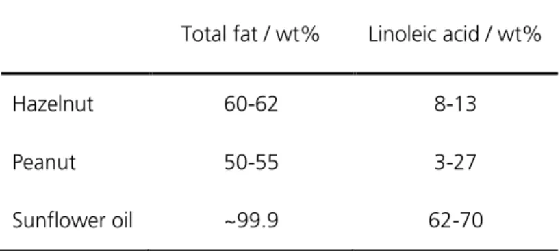
Vegetable oils can generally be separated into pulp and seed oils with olive and palm oil being examples for pulp oils. Sunflower and soy oil in contrast are the main representatives for seed oils.
The group of seed oils also includes oils made from nuts, e.g. hazelnuts or peanuts. 7,8 Besides the importance of cooking oils and oil-containing food for human metabolism quality control of derived products is also a critical issue. Unsaturated fatty acids are very susceptible to oxidation which can result in the formation of harmful substances. 9,10 The oxidation of unsaturated fatty acids is in turn triggered by free radicals which can be generated by light, high temperature, enzymatic reactions, and heavy metal ions. Amongst other substances especially aldehydes are generated during such oxidation processes. 3,11 Hexanal and 2,4-decadienal for example are responsible for the typical rancid smell of deteriorated fatty food and thus for a decrease of organoleptic food properties. 7,12 One of the most frequent fatty acids in vegetable oils is linoleic acid. In sunflower oil the content of linoleic acid is about 62-70 wt%. Linoleic acid is a fatty acid with 18 carbon atoms and is twice unsaturated.
especially of linoleic acid have a reduced oxidation and storage stability. Hexanal is a major reaction product generated during oxidation of linoleic acid. The presence of high hexanal concentrations in oxidized fatty foods has been described in many publications so far. 13,14 Due to the good correlation between oxidation state and hexanal concentration, hexanal is often used as an indicator for the quality of vegetable oils. Moreover, hexanal has a relatively low boiling temperature of 130 °C and a high vapor pressure (13 hPa at 25 °C). 15 Therefore, it evaporates fast which enables a convenient detection in the gas phase of food packaging.
Monitoring the rancidity of fatty food before opening a food package is very difficult until now.
Existing methods are all external and are only practicable in laboratories using special equipment.
Colorimetric detection systems, however, provide a promising solution here. When oxidation products such as hexanal are present, they induce a color change of a special indicator dye which can be immobilized in the food packaging. Thus the oxidation state of fats is easily visualized by the naked eye and as a result consumers can control the food quality before purchasing a certain product.
1.1 Autoxidation of fatty acids
Lipid peroxidation
The main components of vegetable oils and animal fats are triacylglycerides. Triacylglycerides contain of a glycerol backbone which is esterified by fatty acids. 16 In general it can be distinguished between saturated and unsaturated fatty acids. 12 Unsaturated fatty acids like linoleic acid contain one or more allylgroups in their acyl chain. The number of alternating allylgroups has a great effect on the oxidative fat stability as oxidation rate and induction period are highly dependent on the number of double bonds. More precisely, the relative oxidation rate becomes higher and in turn the induction period shorter with an increasing number of allyl groups. 17 In Table C1 relative oxidation rate and induction periods for autoxidation of stearic-, oleic-, linoleic-, and linolenic acid are shown. Linoleic acid shows a 1200 times higher relative oxidation rate than saturated stearic acid. Furthermore, the induction period decreases with an increasing number of double bonds in the alkyl chain of fatty acid. While the induction period of oleic acid is 82 h it is only 19 h for linoleic acid.
Table C1. Correlation between number of double bonds, oxidation rate and induction period of various fatty acids at 25 °C. 7
Fatty acid Number of
allyl groups
Relative oxidation rate
Induction period / h
Stearic acid - 18:0 0 1 n.d.
Oleic acid - 18:1 (9) 1 100 82
Linoleic acid - 18:2 (9, 12) 2 1200 19
Linolenic acid - 18:3 (9, 12, 15) 3 2500 1.34
Autoxidation is a spontaneous reaction of molecular, atmospheric oxygen with lipids. It is a radical chain reaction which includes the three steps initiation, propagation, and termination. 3,7 Formation of initiation radicals (In˙) is provoked by heat, irradiation, enzymatic reactions, or prooxidants like heavy metal ions (Scheme C1). In˙ can subsequently induce hydrogen abstraction from double bonds forming alkyl radicals (R˙). 17,18 The energy barrier for hydrogen abstraction is dependent on the H-atom’s position in the molecule. Dissociation energy for allyl-H-atoms (e.g. in oleic acid) is 322 kJ/mol, whereas energy barrier for abstraction of biallyl-H-atoms (e.g. in linoleic
In In In In
In RH In H R
Scheme C1. Initiation of radical chain reaction by forming initiation radicals (In˙). By H-abstraction from alkyl chain, alkyl radicals (R˙) are generated.
After forming alkyl radicals by CH bond cleavage they further react with oxygen to generate peroxy-radicals (ROO˙, Scheme C2). Peroxy-radicals can react to hydroperoxides (ROOH) by substraction of an allyl-hydrogen radical of an additional fatty acid (Scheme C2). As peroxy- radicals are relatively stable, generation of hydrogenperoxides is the rate limining step of autoxidation reactions. 21
Scheme C2. Propagation step of radical chain reaction by generating peroxy-radicals (ROO˙) which subsequently react with unsaturated fatty acids to form hydroperoxides (ROOH).
Along downstream reactions unstable hydrogen peroxides (ROOH) are decomposed to alkoxy- (RO˙) and hydroxyl-radicals (OH˙). As a result lipid peroxidation is enhanced and the chain reaction is started (Scheme C3). During the reaction course hydroperoxides can accumulate and thus form dimers by hydrogen bonds. Decomposition of these dimers in turn causes the generation of a high amount of peroxy- (ROO˙) and alkoxy- (RO˙) radicals (Scheme C3).
Scheme C3. Decomposition of hydrogen peroxides causes a catalytically speed-up of radical chain reaction.
When oxygen is almost entirely consumed and, therefore, a high concentration of radicals is present, the probability of interaction between two radicals increase. By recombination of radicals to stable non-radical products the radical chain reaction becomes terminated (Scheme C4). 18,22
Scheme C4. Termination of radical chain reaction by forming non-radical products via interaction of two radicals.
The hydroperoxides which are formed in the initial stage of autoxidation are non-volatile, odourless, and relatively unstable. 19 However, by further reaction secondary reaction products like aldehydes, ketones, or alcohols are generated. Especially the resulting carbonyl compounds have a very bad smelling and are therefore responsible for the oxidative or rancid flavor and taste. 22
Time-dependent generation of oxidation products
Autoxidation is a spontaneous process and includes an induction period which is dependent on the number of double bonds in the lipid as well as the atmospheric oxygen concentration.
Furthermore, it is characteristic for the oxidation stability of fatty food. In Figure C1 a schematic time-dependent process of autoxidation is depicted. During the induction period hydroperoxides are generated and thus the oxygen uptake rate is slightly increased. After a certain period of time unstable hydroperoxides decompose to further radicals which results in an autocatalytic speeding up of the oxidation process. As a result the hydroperoxide formation rate decreases after reaching a maximum, whereby the secondary oxidation product and oxygen uptake rates both increase. 22–
24
Figure C1. Time-dependent reaction rates of processes occurring during the autoxidation of fatty acids. 25
Autoxidation of linoleic acid
The relative oxidation rate of linoleic acid is 12 times faster than the oxidation rate of oleic acid (Table C1). This is due to the double-allylic methylen group of linoleic acid 1 at carbon atom 11 which is very reactive to hydrogen abstraction. By abstraction of an H-radical a pentadienyl radical
hydroperoxides 5 and 6 which both contain a conjugated diene-system (Scheme C5). 9,18 In addition, side reactions result also in 8-, 10-, 11-, 12-, and 14-hydroperoxides with an overall yield of 4%. 7,26
Scheme C5. Generation of 9- and 13-hydroperoxides 5 and 6 during autoxidation of linoleic acid 1.
After further reaction steps secondary oxidation products are generated. Table C2 shows their corresponding concentrations after oxidizing 1 g of linoleic acid. 27 The main oxidation product of linoleic acid is hexanal with a concentration of 5100 µg/g. Besides hexanal highly aroma-active compounds like 2,4-decadienal and (E)-2-nonenal were detected in high concentrations as well. 7
Table C2. Volatile compounds generated by autoxidation of 1 g linoleic acid at 20 °C up to an oxygen absorption of 0.5 mol per mol fatty acid. Values were detected using gas chromatography. 7
Oxidation product Concentration /
µg/g Oxidation product Concentration / µg/g
Pentan n.d.* (Z)-3-Nonenal 30
Pentanal 55 (E)-3-Nonenal 30
Hexanal 5100 (Z)-2-Nonenal n.d.
Heptanal 50 (E)-2-Nonenal 30
(E)-2-Heptenal 450 (Z)-2-Dezenal 20
Octenal 45 (E,E)-2,4-Nonadienal 30
1-Octen-3-on 2 (E,Z)-2,4-Decadienal 250
1-Octen-3-
hydroperoxide n.d.* (E,E)-2,4-Decadienal 150
(Z)-2-Octenal 990 Trans-4,5-Epoxy-(E)-2-
decenal n.d.*
(E)-2-Octenal 420
*n.d.: not determined
The reaction steps towards secondary oxidation products formation are shown in Schemes C6- C8. In water-free environment homolytic ß-cleavage of monohydroperoxides is predominant. Here ß-cleavage can take place in two different pathways A and B (Scheme C6). 9 Pathway A is energetically favored whereby hexanal 7 is generated from 13-hydroperoxide 5 (Scheme C7).
Pathway B leads to the formation of pentan, 1-pentanol, and pentanal in this case. In contrast, 9- hydroperoxide 6 predominantly reacts to 2,4-decadienal 9 (pathway B, Scheme C8) besides 2- nonenal (pathway A). 282930
Scheme C6. Reaction pathways for the ß-cleavage of monohydroperoxides whereby volatile secondary oxidation
Scheme C7. Generation of the secondary oxidation products hexanal and 2,4-decadienal from 13- and 9- hydroperoxide.
Additionally, 2,4-decadienal 9 can be further oxidized to hexanal 7 and 2-octenal. 30 This proceeds by the reaction of peroxyradicals (ROO˙) with 9. Thereby, unstable 5- and 3- peroxylperoxides are generated during reaction with oxygen. 5-Peroxylperoxide 12 in turn can decomposes to hexanal whereas 3-peroxylperoxide leads to 2-octenal. The reaction pathway for hexanal formation is shown in Scheme C8.
Scheme C8. Reaction pathway for generation of hexanal from (E,Z)-2,4-decadienal. 29
In summary the concentration of aldehydes and other oxidation products continuously increases during autoxidation of fatty acids for a certain period of time. Beyond a certain point of time, however, the concentration of aldehydes starts to decrease again due to further reaction processes like the oxidation to carboxylic acids. 29,31
1.2 Measuring the autoxidation state of fatty food
For analyzing the oxidation state and the oxidation stability of fatty food many methods were developed in the past. In general these methods can be classified into four categories based on the measured analytes: oxygen absorption, reactant changes, formation of primary and secondary oxidation products, and free radical generation. 30,32 The mentioned methods are further explained in the following.
Since many fatty foods have long induction periods when stored under normal conditions, measuring the autoxidation state of fatty food would take very long. For reducing the analysis time many methods were developed speeding up the oxidation process. E.g. rise of temperature, supply of oxygen, light irradiation, and the addition of catalysts are procedures for activating or supporting the autoxidation process of fatty food. 33
Commonly used testing procedures forecasting storage stabilities of foods include for example the Rancimate test which allows continuous measurement of the induction period. 34 Analyzing the concentration of secondary oxidation products is commonly performed by gas chromatography. Here volatile substances can be quantified by special head-space gas chromatography setups, optionally combined with mass spectrometry. Furthermore, determining of peroxide number, number of dienes, or carbonyl concentration are methods for analyzing the oxidation state of fats. 9,35 Additional, for food industry off-flavor detection by sensory evaluation is a crucial factor. 19,36
The above mentioned methods can provide reasonable information about oxidation states but also suffer from a number of limitations. Autoxidation is a very complex process which can be influenced and changed by complex food matrices or extreme reaction conditions like sample heating for speeding up the oxidation process. 28 Moreover, especially the oxygen absorption rate can lead to wrong values since oxygen consumption is not only caused by fat oxidation but also by oxidation processes of proteins. This can lead to false conclusions about the oxidation state of investigated foods. Hence, for analyzing complex food samples any analysis method has to be selected quite carefully. 36
Measurement of oxygen absorption rate
The oxygen partial pressure has a direct influence on the oxidation stability of fats. Measuring the oxygen absorption rate of foods provides information about their sensitivity towards oxidation. 37 Furthermore, an estimation of the storage stability can be derived. During the
of oxidation process becomes measurable by analyzing oxygen consumption. For a short storage stability of fats in fatty foods a fast increase in oxygen consumption is expected (Figure C2). In contrast, a better storage stability of fats leads to delayed oxygen absorption. Based on this information a comparison of shelf life for different food samples is possible.
Figure C2. Time-depending oxygen consumption indicating the stability of fat-containing foods to oxidation. 25
Oxygen absorption of an investigated fat or food sample can also be measured by mass increase due to oxygen consumption during autoxidation processes. For this purpose the oxidation can be speed up by heating the sample in an oven without air circulation. After certain time intervals the sample is cooled to room temperature and weighed whereby the obtained mass increase reflects the oxidation level of the food sample. The quite simple method can be extended to more sophisticated continuous monitoring of mass and energy changes as well by using thermogravimetry (TG) or differential scanning calorimetry (DSC).
Another method for quantifying oxygen uptakes is the headspace oxygen method which monitors the drop in oxygen pressure. For implementation a sample is placed in a closed vessel containing a certain concentration of oxygen at high temperature (usually around 100 °C). The drop of oxygen pressure is then continuously measured and recorded by an automatic detection unit (e.g. commercial Oxidograph by Mikrolab, Denmark). Pressure changes in the reaction vessel are electronically measured by pressure transducers here.
Alternatively oxygen reduction in the headspace of samples can be measured electrochemically using e.g. a Clark-electrode (galvanic sensor). The possibility of determining the oxidation process without any additional sample treatment like extraction or milling is considered as a big advantage for oxygen measurement methods.