Exercises to Wissenschaftliches Rechnen I/Scientific Computing I (V3E1/F4E1)
Winter 2016 / 17
Prof. Dr. Martin Rumpf
Alexander Effland — Stefanie Heyden — Stefan Simon — Sascha Tölkes
Problem sheet 11
Please hand in the solutions on Tuesday January 24 !
Exercise 35 4 Points
Let Ω ⊂ R 2 be a bounded domain with polygonal boundary and T h be any triangula- tion on Ω. Consider the Raviart-Thomas space RT 0 ( Ω ) given by
RT 0 ( Ω ) = n q ∈ L 2 ( Ω ) : for all T ∈ T h there exists a ∈ R 2 , b ∈ R such that q ( x ) = a + bx for all x ∈ T , [ q ] E · n E = 0 for all E ∈ E h o .
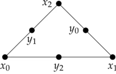
Here, E h is the set of all edges, n E denotes the outer normal of T and [ q ] E refers to the jump along E ∈ E h . Derive an explicit formula for the basis functions of RT 0 using the notation in Figure 1 .
x 0 x 1
x 2
y 2 y 1
y 0
Figure 1 : Triangle with vertices and edge midpoints.
Exercise 36 6 Points For n ∈ N let Ω ⊂ R n be a bounded domain with Lipschitz boundary. Consider the bilinear forms associated with the Stokes equation
a : V × V → R , a ( u, v ) = Z
Ω
∑ n i = 1
∇ u i · ∇ v i dx , b : V × W → R , b ( v, q ) = −
Z
Ω ( divv ) · q dx , where V = H 0 1 ( Ω, R n ) and W = { q ∈ L 2 ( Ω, R n ) : R
Ω q dx = 0 } . Furthermore, we introduce
˜
a : V × V → R , a ˜ ( u, v ) = 2 Z
Ω
∑ n i,j = 1
e ij ( u ) e ij ( v ) dx
with e ij ( u ) = 1 2 ( ∂ j u i + ∂ i u j ) . Prove that a ( u, v ) = a ˜ ( u, v ) for all u, v ∈ { f ∈ V : b ( f , q ) = 0 for all q ∈ W } .
Exercise 37 4 Points
Let Ω ⊂ R 2 be a bounded domain with polygonal boundary and T h a triangulation on Ω. Let V h = RT 0 ( Ω, R 2 ) (see exercise 35 ) and W h ⊂ { f ∈ L 2 ( Ω, R 2 ) : R
Ω f dx = 0 } be any finite-dimensional function space. Furthermore, we set
b : V h × W h → R , b ( v, w ) = − Z
Ω ( divv ) · w dx . Show that (see exercise 33 for the definition of k · k H ( div ) )
w inf ∈ W
hsup
v ∈ V
h| b ( v, w )|
k v k H ( div ) k w k L
2( Ω )
= 0
already implies that there exists w ∈ W h \{ 0 } such that b ( v, w ) = 0 for all v ∈ V h .
Exercise 38 6 Points Let Ω ⊂ R n be a polygonal domain, T h be triangulation of Ω, f ∈ L 2 ( Ω, R 2 ) , and I h be the Lagrange interpolation operator w.r.t. the nodes of T h . To discretize the Stokes equation (see exercise 36 ), we consider the finite element spaces
V h = { v h ∈ C 0 ( Ω, R n ) : v h ∈ P 1 ( T ) ∀ T ∈ T h , v h
∂Ω = 0 } , W h =
p h : Ω → R n : p h ∈ P 0 ( T ) ∀ T ∈ T h , Z
Ω p h dx = 0
. Then we solve the saddle point problem
a ( u h , v h ) + b ( v h , p h ) = (I h ( f ) , v h ) 0,2 ∀ v h ∈ V h , b ( u h , q h ) = 0 ∀ q h ∈ W h . (i.) Construct a basis of W h .
(ii.) Show that solving the saddle point problem corresponds to solving a linear system
A B B T 0
U P
= F
0
. ( 1 )
Derive the matrix representation of A and B.
(iii.) Prove that the sequence ( U ( k ) , P ( k ) ) obtained with Algorithm 1 converges to the solution ( U, P ) of ( 1 ) if THRESHOLD = 0.
Algorithm 1: Saddle point based algorithm.
Data: P
(0), α ∈ ( 0,
kBA−21BTk) , THRESHOLD ≥ 0
1
Set k : = 1;
2
repeat
3
Solve AU
(k): = F − B
TP
(k−1);
4
Set P
(k): = P
(k−1)+ αBU
(k);
5
Set k : = k + 1;
6