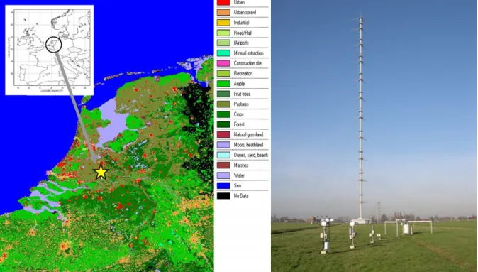
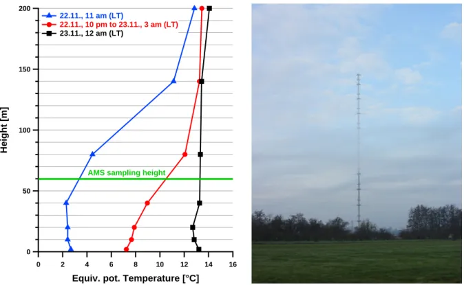
Measurements at the CESAR Tower at Cabauw, NL
237
0
0
Volltext
(2)
(3)
(4)
(5)
(6)
(7)
(8)(9)
(10)
(11)
(12)
(13)
(14)
(15)
(16)
(17)
(18)
(19)
(20)
(21)
(22)
(23)
(24)
(25)
(26)
(27)
(28)
(29)
(30)
(31)
Abbildung
+7

ÄHNLICHE DOKUMENTE
Eine Messung der Polarisation im Endzustand ist experimentell nur f¨ur t-Leptonen m¨oglich, da man deren Spin aus der Winkelverteilung der Produkte von t-Zerf¨allen bestimmen kann..
If the distribution function is presented on wide logarithmic scale then an intelligible measure of the mobility resolution is the number of Resolved Fractions Per Decade
Correlation between total ion mass from the TNy samples and particle volume concentration calculated from the Grimm OPC measurements.
Sun photometer measurements both in Ny- Ålesund and at the Zeppelin station as well as Ceilometer (Vaisala CL51) profiles have been employed to improve the evaluation of KARL data
Statistical theories regu- larly end in closure problems, which require the ad-hoc assumption of closure models (see. The turbulence problem could therefore be described as a quest
In order to investigate the effect of the high surface albedo prevailing on an Antarctic ice shelf on various downwelling radiation parameters, the Institute of Meteorology
Comparison of lidar (black) and radiosonde (blue) measurements of water vapor (in terms of the relative humidity).. Up to the thin cirrus cloud in 8.5 km altitude the measurements
Summary: As part of a [arger experimcut , atmospheric turbidity measurements were carried out during the austral summer 1985/86 in Ade- lie Land, Eastcrn Antarctica at 1560
