arXiv:1101.2082v2 [astro-ph.HE] 12 Jan 2011
Detection of a spectral break in the extra hard component of GRB 090926A
M. Ackermann
2, M. Ajello
2, K. Asano
3, M. Axelsson
4,5,6, L. Baldini
7, J. Ballet
8, G. Barbiellini
9,10, M. G. Baring
11, D. Bastieri
12,13, K. Bechtol
2, R. Bellazzini
7, B. Berenji
2,
P. N. Bhat
14, E. Bissaldi
15, R. D. Blandford
2, E. Bonamente
16,17, A. W. Borgland
2, A. Bouvier
2, J. Bregeon
7,1, A. Brez
7, M. S. Briggs
14, M. Brigida
18,19, P. Bruel
20, R. Buehler
2, S. Buson
12,13, G. A. Caliandro
21, R. A. Cameron
2, P. A. Caraveo
22, S. Carrigan
13, J. M. Casandjian
8, C. Cecchi
16,17, ¨ O. C ¸ elik
23,24,25, V. Chaplin
14, E. Charles
2,
A. Chekhtman
26,27, J. Chiang
2, S. Ciprini
17, R. Claus
2, J. Cohen-Tanugi
28, V. Connaughton
14, J. Conrad
29,6,30, S. Cutini
31, C. D. Dermer
26, A. de Angelis
32,
F. de Palma
18,19, B. L. Dingus
33, E. do Couto e Silva
2, P. S. Drell
2, R. Dubois
2, C. Favuzzi
18,19, S. J. Fegan
20, E. C. Ferrara
23, W. B. Focke
2, M. Frailis
32,34, Y. Fukazawa
35,
S. Funk
2, P. Fusco
18,19, F. Gargano
19, D. Gasparrini
31, N. Gehrels
23, S. Germani
16,17, N. Giglietto
18,19, F. Giordano
18,19, M. Giroletti
36, T. Glanzman
2, G. Godfrey
2, A. Goldstein
14,1, J. Granot
37, J. Greiner
15, I. A. Grenier
8, J. E. Grove
26, S. Guiriec
14, D. Hadasch
21, Y. Hanabata
35, A. K. Harding
23, K. Hayashi
35, M. Hayashida
2, E. Hays
23, D. Horan
20, R. E. Hughes
38, R. Itoh
35, G. J´ohannesson
2, A. S. Johnson
2, W. N. Johnson
26,
T. Kamae
2, H. Katagiri
35, J. Kataoka
39, R. M. Kippen
33, J. Kn¨odlseder
40, D. Kocevski
2, C. Kouveliotou
41, M. Kuss
7, J. Lande
2, L. Latronico
7, S.-H. Lee
2, M. Llena Garde
29,6,
F. Longo
9,10, F. Loparco
18,19, M. N. Lovellette
26, P. Lubrano
16,17, A. Makeev
26,27, M. N. Mazziotta
19, S. McBreen
15,42, J. E. McEnery
23,43, S. McGlynn
44,6, C. Meegan
45, J. Mehault
28, P. M´esz´aros
46, P. F. Michelson
2, T. Mizuno
35, C. Monte
18,19, M. E. Monzani
2, E. Moretti
44,6, A. Morselli
47, I. V. Moskalenko
2, S. Murgia
2, H. Nakajima
48, T. Nakamori
39,
M. Naumann-Godo
8, S. Nishino
35, P. L. Nolan
2, J. P. Norris
49, E. Nuss
28, M. Ohno
50, T. Ohsugi
51, A. Okumura
50, N. Omodei
2, E. Orlando
15, J. F. Ormes
49, M. Ozaki
50, W. S. Paciesas
14, D. Paneque
2, J. H. Panetta
2, D. Parent
26,27, V. Pelassa
28, M. Pepe
16,17, M. Pesce-Rollins
7, V. Petrosian
2, F. Piron
28, T. A. Porter
2, R. Preece
14,1, J. L. Racusin
23,
S. Rain`o
18,19, R. Rando
12,13, A. Rau
15, M. Razzano
7, S. Razzaque
26,52, A. Reimer
53,2, O. Reimer
53,2, T. Reposeur
54, L. C. Reyes
55, J. Ripken
29,6, S. Ritz
56, M. Roth
57, F. Ryde
44,6, H. F.-W. Sadrozinski
56, A. Sander
38, J. D. Scargle
58, T. L. Schalk
56, C. Sgr`o
7,
E. J. Siskind
59, P. D. Smith
38, G. Spandre
7, P. Spinelli
18,19, M. Stamatikos
23,38, F. W. Stecker
23, M. S. Strickman
26, D. J. Suson
60, H. Tajima
2, H. Takahashi
51,1, T. Tanaka
2, Y. Tanaka
50, J. B. Thayer
2, J. G. Thayer
2, L. Tibaldo
12,13,8,61, D. Tierney
42,
K. Toma
46,1, D. F. Torres
21,62, G. Tosti
16,17, A. Tramacere
2,63,64, Y. Uchiyama
2,
T. Uehara
35,1, T. L. Usher
2, J. Vandenbroucke
2, A. J. van der Horst
41,65, V. Vasileiou
24,25,
N. Vilchez
40, V. Vitale
47,66, A. von Kienlin
15, A. P. Waite
2, P. Wang
2, C. Wilson-Hodge
41, B. L. Winer
38, K. S. Wood
26, X. F. Wu
46,67,68, R. Yamazaki
69, Z. Yang
29,6, T. Ylinen
44,70,6,
M. Ziegler
561
Corresponding authors: J. Bregeon, johan.bregeon@pi.infn.it; A. Goldstein, amg0005@uah.edu;
R. Preece, Rob.Preece@nasa.gov; H. Takahashi, hirotaka@hep01.hepl.hiroshima-u.ac.jp; K. Toma, toma@astro.psu.edu; T. Uehara, uehara@hep01.hepl.hiroshima-u.ac.jp.
2
W. W. Hansen Experimental Physics Laboratory, Kavli Institute for Particle Astrophysics and Cosmol- ogy, Department of Physics and SLAC National Accelerator Laboratory, Stanford University, Stanford, CA 94305, USA
3
Interactive Research Center of Science, Tokyo Institute of Technology, Meguro City, Tokyo 152-8551, Japan
4
Department of Astronomy, Stockholm University, SE-106 91 Stockholm, Sweden
5
Lund Observatory, SE-221 00 Lund, Sweden
6
The Oskar Klein Centre for Cosmoparticle Physics, AlbaNova, SE-106 91 Stockholm, Sweden
7
Istituto Nazionale di Fisica Nucleare, Sezione di Pisa, I-56127 Pisa, Italy
8
Laboratoire AIM, CEA-IRFU/CNRS/Universit´e Paris Diderot, Service d’Astrophysique, CEA Saclay, 91191 Gif sur Yvette, France
9
Istituto Nazionale di Fisica Nucleare, Sezione di Trieste, I-34127 Trieste, Italy
10
Dipartimento di Fisica, Universit`a di Trieste, I-34127 Trieste, Italy
11
Rice University, Department of Physics and Astronomy, MS-108, P. O. Box 1892, Houston, TX 77251, USA
12
Istituto Nazionale di Fisica Nucleare, Sezione di Padova, I-35131 Padova, Italy
13
Dipartimento di Fisica “G. Galilei”, Universit`a di Padova, I-35131 Padova, Italy
14
Center for Space Plasma and Aeronomic Research (CSPAR), University of Alabama in Huntsville, Huntsville, AL 35899, USA
15
Max-Planck Institut f¨ ur extraterrestrische Physik, 85748 Garching, Germany
16
Istituto Nazionale di Fisica Nucleare, Sezione di Perugia, I-06123 Perugia, Italy
17
Dipartimento di Fisica, Universit`a degli Studi di Perugia, I-06123 Perugia, Italy
18
Dipartimento di Fisica “M. Merlin” dell’Universit`a e del Politecnico di Bari, I-70126 Bari, Italy
19
Istituto Nazionale di Fisica Nucleare, Sezione di Bari, 70126 Bari, Italy
20
Laboratoire Leprince-Ringuet, ´ Ecole polytechnique, CNRS/IN2P3, Palaiseau, France
21
Institut de Ciencies de l’Espai (IEEC-CSIC), Campus UAB, 08193 Barcelona, Spain
22
INAF-Istituto di Astrofisica Spaziale e Fisica Cosmica, I-20133 Milano, Italy
23
NASA Goddard Space Flight Center, Greenbelt, MD 20771, USA
24
Center for Research and Exploration in Space Science and Technology (CRESST) and NASA Goddard
Space Flight Center, Greenbelt, MD 20771, USA
25
Department of Physics and Center for Space Sciences and Technology, University of Maryland Baltimore County, Baltimore, MD 21250, USA
26
Space Science Division, Naval Research Laboratory, Washington, DC 20375, USA
27
George Mason University, Fairfax, VA 22030, USA
28
Laboratoire de Physique Th´eorique et Astroparticules, Universit´e Montpellier 2, CNRS/IN2P3, Mont- pellier, France
29
Department of Physics, Stockholm University, AlbaNova, SE-106 91 Stockholm, Sweden
30
Royal Swedish Academy of Sciences Research Fellow, funded by a grant from the K. A. Wallenberg Foundation
31
Agenzia Spaziale Italiana (ASI) Science Data Center, I-00044 Frascati (Roma), Italy
32
Dipartimento di Fisica, Universit`a di Udine and Istituto Nazionale di Fisica Nucleare, Sezione di Trieste, Gruppo Collegato di Udine, I-33100 Udine, Italy
33
Los Alamos National Laboratory, Los Alamos, NM 87545, USA
34
Osservatorio Astronomico di Trieste, Istituto Nazionale di Astrofisica, I-34143 Trieste, Italy
35
Department of Physical Sciences, Hiroshima University, Higashi-Hiroshima, Hiroshima 739-8526, Japan
36
INAF Istituto di Radioastronomia, 40129 Bologna, Italy
37
Centre for Astrophysics Research, Science and Technology Research Institute, University of Hertford- shire, Hatfield AL10 9AB, UK
38
Department of Physics, Center for Cosmology and Astro-Particle Physics, The Ohio State University, Columbus, OH 43210, USA
39
Research Institute for Science and Engineering, Waseda University, 3-4-1, Okubo, Shinjuku, Tokyo, 169-8555 Japan
40
Centre d’´ Etude Spatiale des Rayonnements, CNRS/UPS, BP 44346, F-30128 Toulouse Cedex 4, France
41
NASA Marshall Space Flight Center, Huntsville, AL 35812, USA
42
University College Dublin, Belfield, Dublin 4, Ireland
43
Department of Physics and Department of Astronomy, University of Maryland, College Park, MD 20742, USA
44
Department of Physics, Royal Institute of Technology (KTH), AlbaNova, SE-106 91 Stockholm, Sweden
45
Universities Space Research Association (USRA), Columbia, MD 21044, USA
46
Department of Astronomy and Astrophysics, Pennsylvania State University, University Park, PA 16802, USA
47
Istituto Nazionale di Fisica Nucleare, Sezione di Roma “Tor Vergata”, I-00133 Roma, Italy
ABSTRACT
We report on the observation of the bright, long gamma-ray burst, GRB 090926A, by the Gamma-ray Burst Monitor (GBM) and Large Area Tele-
48
Department of Physics, Tokyo Institute of Technology, Meguro City, Tokyo 152-8551, Japan
49
Department of Physics and Astronomy, University of Denver, Denver, CO 80208, USA
50
Institute of Space and Astronautical Science, JAXA, 3-1-1 Yoshinodai, Sagamihara, Kanagawa 229-8510, Japan
51
Hiroshima Astrophysical Science Center, Hiroshima University, Higashi-Hiroshima, Hiroshima 739-8526, Japan
52
National Research Council Research Associate, National Academy of Sciences, Washington, DC 20001, USA
53
Institut f¨ ur Astro- und Teilchenphysik and Institut f¨ ur Theoretische Physik, Leopold-Franzens- Universit¨at Innsbruck, A-6020 Innsbruck, Austria
54
Universit´e Bordeaux 1, CNRS/IN2p3, Centre d’´ Etudes Nucl´eaires de Bordeaux Gradignan, 33175 Gradignan, France
55
Kavli Institute for Cosmological Physics, University of Chicago, Chicago, IL 60637, USA
56
Santa Cruz Institute for Particle Physics, Department of Physics and Department of Astronomy and Astrophysics, University of California at Santa Cruz, Santa Cruz, CA 95064, USA
57
Department of Physics, University of Washington, Seattle, WA 98195-1560, USA
58
Space Sciences Division, NASA Ames Research Center, Moffett Field, CA 94035-1000, USA
59
NYCB Real-Time Computing Inc., Lattingtown, NY 11560-1025, USA
60
Department of Chemistry and Physics, Purdue University Calumet, Hammond, IN 46323-2094, USA
61
Partially supported by the International Doctorate on Astroparticle Physics (IDAPP) program
62
Instituci´ o Catalana de Recerca i Estudis Avan¸cats (ICREA), Barcelona, Spain
63
Consorzio Interuniversitario per la Fisica Spaziale (CIFS), I-10133 Torino, Italy
64
INTEGRAL Science Data Centre, CH-1290 Versoix, Switzerland
65
NASA Postdoctoral Program Fellow, USA
66
Dipartimento di Fisica, Universit`a di Roma “Tor Vergata”, I-00133 Roma, Italy
67
Joint Center for Particle Nuclear Physics and Cosmology (J-CPNPC), Nanjing 210093, China
68
Purple Mountain Observatory, Chinese Academy of Sciences, Nanjing 210008, China
69
Aoyama Gakuin University, Sagamihara-shi, Kanagawa 229-8558, Japan
70
School of Pure and Applied Natural Sciences, University of Kalmar, SE-391 82 Kalmar, Sweden
scope (LAT) instruments on board the Fermi Gamma-ray Space Telescope.
GRB 090926A shares several features with other bright LAT bursts. In par- ticular, it clearly shows a short spike in the light curve that is present in all detectors that see the burst, and this in turn suggests that there is a common region of emission across the entire Fermi energy range. In addition, while a separate high-energy power-law component has already been observed in other GRBs, here we report for the first time the detection with good significance of a high-energy spectral break (or cutoff) in this power-law component around 1.4 GeV in the time-integrated spectrum. If the spectral break is caused by opac- ity to electron-positron pair production within the source, then this observation allows us to compute the bulk Lorentz factor for the outflow, rather than a lower limit.
Subject headings: gamma rays: bursts
1. Introduction
Gamma-Ray Bursts (GRBs) are the most energetic transients in the universe. The first brief and intense flash, the so-called prompt emission, has been observed in the X-ray and gamma-ray bands, while subsequent long-lived afterglow emission has so far been observed mainly at energies in the X-ray band and below. The prompt emission is thought to be produced in an ultra-relativistic outflow, but its detailed emission mechanism has been a long- standing problem. It has been widely believed that the afterglow is the synchrotron emission from the forward shock that propagates in the external medium, but Swift observations have pointed out some difficulties in this model (for recent reviews, Zhang 2007; M´esz´aros 2006). The study of the gamma-ray emission in the GeV energy range is expected to give us important information on these issues and even on the nature of the progenitors and the ultra-relativistic outflows of GRBs (Band et al. 2009; Falcone et al. 2008; Fan & Piran 2008).
The Fermi Gamma-ray Space Telescope hosts two instruments, the Large Area Tele-
scope (LAT, 20 MeV to more than 300 GeV; Atwood et al. 2009) and the Gamma-ray Burst
Monitor (GBM, 8 keV–40 MeV; Meegan et al. 2009), which together are capable of measur-
ing the spectral parameters of GRBs across seven decades in energy. Since the start of science
operations in early August 2008, the Fermi LAT has significantly detected 16 GRBs. These
events, including the very bright long-duration and short-duration bursts GRB 080825C,
GRB 080916C, GRB 081024B, GRB 090510, and GRB 090902B, have revealed many im-
portant, seemingly common, features of GRB GeV emission (Abdo et al. 2009a,b,c,d, 2010;
Ackermann et al. 2010a,b): (1) the GeV emission onsets of many LAT GRBs are delayed with respect to the MeV emission onsets; (2) some LAT GRBs have extra hard components apart from the canonical Band function (Band et al. 1993), which typically peaks in νF
νbetween around 100 keV–1 MeV; (3) the GeV emission lasts longer than the prompt MeV emission, showing power-law temporal decays at late times.
In this paper, we report on the analysis of the bright, long GRB 090926A detected by Fermi LAT/GBM. The light curve of this burst above 100 MeV shows a sharp spike with a width of 0.15 s, fast variability that we use to constrain the origin of the high-energy photons within the spike. Furthermore, from the detection of a break in the > 100 MeV gamma-ray spectrum, we derive constraints on the bulk Lorentz factor and the distance of the emitting region from the central source. Section 2 summarizes the detections of GRB 090926A by the GBM and the LAT, and the follow-up observations. Section 3 presents the light curves of the prompt emission as seen by both instruments and describes a sharp pulse seen in all detectors.
In section 4, we detail the spectral analysis of the burst through time-resolved spectroscopy, the measurement of a break in the extra-component, and the extended emission found in the LAT data out to 4.8 ks after the trigger. These last two points are at the center of the physical interpretation of the observations that is developed in section 5.1. Throughout this paper, we adopt a Hubble constant of H
0= 72 km s
−1Mpc
−1and cosmological parameters of Ω
Λ= 0.73 and Ω
M= 0.27.
2. Observations
At 04:20:26.99 (UT) on Sept. 26, 2009 (hereafter T
0= 275631628.98 s mission elapsed time), the Fermi Gamma-ray Burst Monitor (GBM) triggered on and localized the long GRB 090926A at (RA, Dec) = (354.5
◦, −64.2
◦), in J2000 coordinates (Bissaldi 2009; Uehara et al.
2009). This position was ∼52
◦with respect to the LAT boresight at the time of the trigger and well within the field of view. An Autonomous Repoint Request (ARR) was gener- ated, but the spacecraft initially remained in survey mode as the Earth avoidance angle condition was not satisfied by the burst pointing direction. The on-board GBM position of GRB 090926A was occulted by the Earth at roughly T
0+ 500 s until it rose above the horizon at approximately T
0+ 3000 s. At that time, the spacecraft slewed to GRB 090926A and kept it close to the center of the LAT field of view until T
0+ 18000 s, though the source location was occulted by the Earth several times over that time period.
Emission from GRB 090926A was evident in the Fermi LAT raw trigger event rates, and
the number of LAT events (∼ 200 photon candidates above 100 MeV) is comparable to that of
the other bright LAT bursts, GRB 080916C, GRB 090510 and GRB 090902B. The increase
in the photon count rate during the prompt phase is spatially and temporally correlated with the GBM emission with high significance, and extended emission is observed until T
0+ 4800 s. The best LAT on-ground localization is (RA, Dec) = (353.56
◦, −66.34
◦), with a 90% containment radius of 0.07
◦(statistical; 68% containment radius: 0.04
◦, systematic error is less than 0.1
◦) and is consistent with the XRT localization.
Indeed, based upon the GCN report issued for the LAT detection, a Swift TOO ob- servation was performed, and an afterglow for GRB 090926A was detected with XRT and UVOT at T
0+ 47 ks and localized at (RA, Dec) = (353.40070
◦, -66.32390
◦) with an uncer- tainty of 1.5
′′(90% confidence) (Vetere et al. 2009). VLT observations determined a redshift for GRB 090926A of z = 2.1062, using the X-shooter spectrograph (Malesani et al. 2009).
Suzaku/WAM and Skynet/PROMPT also detected the soft gamma-ray prompt and optical afterglow emission, respectively (Noda et al. 2009).
3. Light Curves
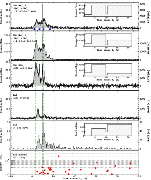
In figure 1, we show the GBM and LAT light curves in several energy bands. The highest energy photon is a 19.6 GeV event, observed at T
0+ 25 s within 0.03
◦from the LAT position of GRB 090926A, well within the 68% containment of the point spread function at that energy. The light curves show that the onset of the LAT emission is delayed by 3.3 s with respect to the GBM emission, similar to other LAT GRBs (Abdo et al. 2009a,b,c,d, 2010; Ackermann et al. 2010a,b). Detailed analysis of the GBM data results in a formal T90 duration
1(Kouveliotou et al. 1993) of 13.1 ± 0.2 s, with a start time of T
0+ 2.2 s and a stop time of T
0+ 15.3 s. The emission measured in the LAT above 100 MeV has a similar duration; however, owing to the efficient background rejection applied to the LAT data, the signal is clearly visible in the light curve well after this time range.
The time intervals chosen for spectroscopy are indicated by the vertical lines in figure 1, with boundaries at T
0+(0, 3.3, 9.8, 10.5, 21.6) s. The end of the last time interval at T
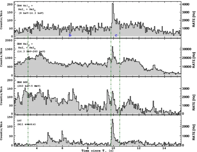
0+21.6 s was chosen somewhat arbitrarily as the end of the prompt phase, but we carefully verified that our results are not affected by a slightly different choice. Figure 2 shows a zoom of some of the light curves between T
0+ 2.2 s and T
0+ 15.3 s, with a binning of 0.05 s, and highlights the presence of the sharp peak seen in each of the NaI, BGO, and LAT light curves at T
0+ 10 s. As seen on figure 2, the peak is clearly in coincidence in all of the light curves, indicating a strong correlation of the emission from a few keV to energies > 100
1
The T90 duration is the time over which the central 90% of the counts between 50 and 300 keV have
been accumulated.
MeV. Because this peak is the only one evident at all energies, we chose to run a dedicated spectral analysis between T
0+ 9.8 s and T
0+ 10.5 s as described in section 4.1.
We estimated the variability time scale using the full width at half maximum (FWHM) of the bright pulse seen around T
0+ 10 s. A combination of exponential functions is used to fit the light curve as performed in Norris et al. (1996). The light curve fitting is performed for all bright NaI detectors (N6, N7, N8) with a 2 ms time resolution. Two exponential functions are used to represent the weak and main bright peaks and include a quadratic function to fit the longer timescale variations. As a result, we obtain a FWHM of the main peak of 0.15 ± 0.01 s for the bright pulse.
4. Spectral Analysis
4.1. LAT and GBM spectral fitting
We performed a time-integrated joint spectral analysis of the LAT and GBM data for the prompt phase defined as T
0+ 3.3 s to T
0+ 21.6 s in figure 1. For the GBM, we used
‘Time Tagged Events’ (TTE) data from the NaI detectors 6, 7, 8 and BGO detector 1. As in Abdo et al. (2009d), background rates and errors are estimated during the prompt phase by fitting background regions of the light curve before and after the burst. We derived our background estimates using the time intervals [T
0− 44; T
0− 8] s and [T
0+ 36; T
0+ 100] s for the NaI detectors, and [T
0− 43; T
0− 16] s and [T
0+ 43; T
0+ 300] s for the BGO detector.
For the LAT, we extracted ‘transient’ class data from an energy-dependent acceptance cone around the burst position, as described in Abdo et al. (2009d), and considered front- and back-converting events separately (Atwood et al. 2009). The data files for the analysis were prepared using the LAT ScienceTools-v9r15p2 package, which is available from the Fermi Science Support Center (FSSC), and the P6 V3 TRANIENT response functions.
71A synthetic background was derived for the LAT data using an empirical model of the rates expected for the position of the source in the sky and for the position and orientation of the spacecraft during the burst interval.
The joint spectral fitting of GBM and LAT data was performed using rmfit version 3.2 (Kaneko et al. 2006; Abdo et al. 2009d), which estimates the goodness-of-fit in terms of the Castor Statistic (C-STAT) to handle correctly the small number of events at the highest energies. The Castor statistic (Dorman 2003) is similar to the Cash statistic (Cash 1979) except for an offset that is constant for a particular dataset. A global effective area correction
71
http://fermi.gsfc.nasa.gov/ssc/
-20 0 20 40 60 80 100
Counts/Bin
0 100 200 300 400
RATE [Hz]
0 1000 2000 3000 4000
a a b a b c a b c d
6 + GBM NaI
+ NaI8 NaI7
(8 keV-14.3 keV)
0 (s) Time since T
5 10 15 20
Counts/bin 0
2000 4000 6000
-20 0 20 40 60 80 100
Counts/Bin
0 1000 2000 3000
RATE [Hz]
0 10000 20000
6 + GBM NaI
+ NaI8 NaI7
(14.3 keV-260 keV)
0 (s) Time since T
5 10 15 20
Counts/bin 0
50000 100000
-20 0 20 40 60 80 100
Counts/Bin
0 100 200 300
RATE [Hz]
0 1000 2000 GBM BGO1
(260 keV-5 MeV)
0 (s) Time since T
5 10 15 20
Counts/bin 0
5000 10000
-20 0 20 40 60 80 100
Counts/Bin
0 100 200
RATE [Hz]
0 1000 2000 LAT
(All events)
-20 0 20 40 60 80 100
Counts/Bin
0 10 20 30
RATE [Hz]
0 20 40 60 LAT
(> 100 MeV)
0 (s) Time since T
5 10 15 20
Counts/bin 0
50 100
0 (s) Time since T
-20 0 20 40 60 80 100
Energy [MeV]
103
104
LAT EVENTS (> 1 GeV)
Fig. 1.— GBM and LAT light curves for the gamma-ray emission of GRB 090926A. The data from the GBM NaI detectors were divided into soft (8–14.3 keV) and hard (14.3–
260 keV) bands to reveal similarities between the light curve at the lowest energies and that
of the LAT data. The fourth panel shows all LAT events that pass the on-board GAMMA
filter (Atwood et al. 2009). The first four light curves are background-subtracted and are
shown for 0.1 s time bins. The fifth and sixth panels show LAT data ‘transient’ class events
for energies > 100 MeV and > 1 GeV respectively, both using 0.5 s time bins. The vertical
lines indicate the boundaries of the intervals used for the time-resolved spectral analysis,
T
0+ (0, 3.3, 9.8, 10.5, 21.6) s. The insets show the counts for each data set, binned using
these intervals, to illustrate the numbers of counts considered in each spectral fit.
Fig. 2.— GBM and LAT light curves for the gamma-ray emission of GRB 090926A with
0.05 s time binning for the core of the prompt phase. The vertical dashed lines at T
0+ 9.8 s
and T
0+ 10.5 s define interval c used in the spectral analysis, see section 4.1.
has been applied to the BGO data to match the model normalizations given by the NaI data;
this correction is consistent with the relative uncertainties in the GBM detector responses.
Uncorrected, this will normally cause a mismatch between the fitted model rates between the two types of detectors where they overlap in energy. Once the correction has been determined, it is held fixed throughout the calculation, since it reflects an uncertainty in the response rather than in the data. In this analysis, the NaI to BGO normalization factor was found to be 0.79. For further details on the data extraction and spectral analysis procedures see our previous publications Abdo et al. (2009d) and Abdo et al. (2010).
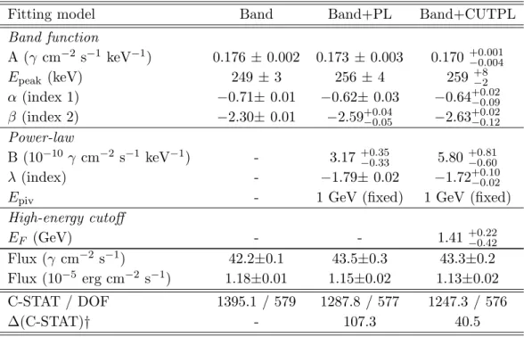
Initially, we fitted a canonical Band function (Band et al. 1993) to the data and then found that adding an extra power-law component improved both the fit statistics and residu- als. Table 1 summarizes the best-fit parameters and shows that the improvement in C-STAT for the (Band+PL) fit over the Band fit alone is 107.3, indicating a firm detection of the additional power-law component. The parameters of the Band function are stable, and the power-law photon index of the additional component is λ = −1.79 ± 0.02.
In order to better characterize the power-law component at the highest energies, we ran a LAT-only data analysis using the unbinned likelihood technique for the full prompt phase. The fitted spectrum is shown in figure 3 (black points). The resulting photon index is −2.29 ± 0.09, much softer than the −1.79 ± 0.02 index found for the joint GBM/LAT analysis. Considering the systematic effects in both analyses, this difference in photon index is significant (∼ 3σ level) and is an indication of the presence of a spectral break. With the LAT data alone, we could not find any significant evidence for a deviation from the simple power-law shape, probably because of the limited lever arm in energy. Hence, we investigated this effect using the joint fits of the GBM and LAT data.
We fitted the GBM/LAT spectra with the combination of the Band function and a power-law model with an exponential cutoff (CUTPL),
f(E) = B E
E
piv λexp
− E E
F. (1)
Here B is the normalization in units of photons s
−1cm
−2keV
−1, E
pivis the pivot energy fixed at 1 GeV, E
Fis the e-folding energy, and λ is the power-law photon index.
The fit results are summarized in table 1, and the count spectra and residuals are
shown in figure 4 for the best-fit model. The e-folding energy is E
F= 1.41
+0.22−0.42stat. ±
0.30 syst. GeV, while the power-law photon index below the cutoff energy is λ ≃ −1.72
+0.10−0.02stat. ±
0.01 syst., which is a bit harder than in the (Band+PL) case. The systematic uncertainties
have been derived using the bracketing instrument response functions, as described in detail
in Abdo et al. (2009d). The parameters of the Band function change little from one fit to
another. The C-STAT value for this model improves by 40.5 compared to the (Band+PL) model, which is significant at the > 4σ level (see the deeper discussion below). We also tried to fit the data with a broken power-law model,
f(E) =
C
E Epiv
λlfor E ≤ E
breakC
Ebreak
Epiv
λlE Ebreak
λhfor E > E
break
, (2)
where λ
land λ
hare the low- and high-energy power-law photon indexes, respectively, E
pivis the pivot energy fixed at 1 GeV, and E
breakis the break energy. However, the significance of the fit was close to that found using the (CUTPL) model so that we cannot distinguish between the two models. The fit with a broken power-law gave a break energy E
break= 219
+65−56MeV and a high-energy photon index of λ
h= −2.47
+0.14−0.17.
One may assess the significance of the spectral cutoff by computing the difference in the best-fit C-STAT values for the (Band+PL) and (Band+CUTPL) models. Since C-STAT is equal to twice the log-likelihood, this is the standard likelihood ratio test; and conventionally, one calculates the significance of a change in log-likelihood using Wilks’ theorem. In this case, Wilks’ theorem states the ∆(C-STAT) values should be asymptotically distributed as χ
2for one degree of freedom. However, certain assumptions are required for the validity of this calculation. For the highest reliability, we studied the distribution of ∆(C-STAT) values via simulations, creating 2 × 10
4random realizations of the null hypothesis (the (Band+PL) model with parameters set at the best-fit values) and fit the data for each trial with both models. In the resulting distribution of ∆(C-STAT) values, the largest difference we found was 16.7, much smaller than the value of 40.5 for the actual data (see table 1). We therefore place a firm upper-limit on the probability that our fit of the exponential cutoff occurred by chance of 5 × 10
−5. This corresponds to a Gaussian equivalent significance of 4.05σ.
Our distribution of ∆(C-STAT) values shows a slight excess over the χ
2distribution at large values indicating that perhaps the asymptotic distribution has not been reached for this number of trials. To be conservative, we do not evaluate the significance according to the conventional procedure of using the observed ∆(C-STAT) value of 40.5 and the χ
2distribution. Unfortunately, the number of simulations that would be required to determine the significance of the observed cutoff is prohibitive. Nonetheless, the sizeable gap between the largest ∆(C-STAT) value obtained in the simulations, 16.7, and the observed value of 40.5 suggests that the significance is much larger than 4σ. For the 4 different sets of instrument response functions that we used in our study of the systematic uncertainties, we always found
∆(C-STAT)≥ 32. The significance of the spectral cutoff will be hereafter quoted as > 4σ.
Using the fit results for the best model (Band+CUTPL), we estimate a fluence of
2.07±0.04 × 10
−4erg cm
−2(10 keV–10 GeV) from T
0+ 3.3 s to T
0+ 21.6 s. These data
give an isotropic energy E
γ,iso= 2.24 ±0.04 × 10
54erg, comparable to that of GRB 090902B (Abdo et al. 2009a).
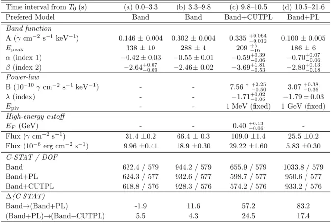
We then performed a time-resolved spectral analysis of the prompt phase in the four time intervals a, b, c, d. The spectra are shown in figure 5, and the results are summarized in table 2, where the best-fit parameters are given for the statistically preferred model, and the C-STAT values are given for the various models. The extra power-law component is found to be very significant in intervals c and d , but not at the beginning of the prompt phase in intervals a and b. The spectral cutoff is significant at the > 4σ level only in the common sharp peak (time interval c ), where the GeV flux is the highest, but is only marginally significant (∼ 4σ) in time bin d.
In time interval b , the improvement in the fit statistics when adding the extra power-law component is only ∆(C-STAT) = 11.6. As a consequence, the parameters of the power-law are not very well constrained, yielding a normalization B = 2.9
+6.4−1.010
−10photons cm
−2s
−1keV
−1and a power-law index λ = 1.7
+0.2−0.1. In time interval c, we found the cutoff energy to be E
F= 0.40
+0.13−0.06stat. ± 0.05 syst. GeV (table 2). Note that we fixed the pivot energy at E
piv= 1 MeV for time interval c, since this is the only interval where the extra power- law component is dominant over the Band component at very low energies, and setting E
piv= 1 GeV resulted in very asymmetric and very large uncertainties, especially for the normalization B of the extra power-law component. We also tried to fit time interval c with a broken power-law model, see equation 2; but again the fit significance was close to that of the (Band+CUTPL) model, so that we cannot distinguish between the two models. The fit with a broken power law gave a break energy E
break= 264
+233−75MeV and a photon index above E
breakof λ
h= −3.55
+0.63−3.28. In time interval d , the improvement in the fit statistics when adding a cutoff to the the extra power-law component is only 17.4 (roughly ∼ 4σ), which is quite high, but not sufficient to claim the presence of an energy cutoff in this bin alone. However, as the cutoff is strong in the preceding time interval c, we looked at the behavior of the e-folding energy. For time interval d, the e-folding energy is found to be E
F= 2.21
+0.92−0.69GeV, which is much higher than the one found in interval c (the 2-σ confidence intervals for the cutoff in bins c and d actually exclude each other). This indicates a possible time evolution of the high energy cutoff.
4.2. LAT extended emission
As the burst was occulted by the Earth from T
0+ 540 s to T
0+ 3000 s, we performed the
unbinned likelihood analysis using ‘transient’ class events in the time interval from T
0+ 20 s
to T
0+ 300 s (a small margin is needed to safely define a circular ROI), and use ‘diffuse’
class events after T
0+ 3000 s
1. ‘Transient’ class events are treated as in §4.1. In addition, for the ‘diffuse’ class events, we included in the model the standard galactic background component, described by the FITS model file gll iem v02.fit, with fixed normalization, and the standard isotropic background component, whose spectrum is given in the model file isotropic iem v02.txt, with the normalization left free. Both model files may be downloaded from the FSSC website.
We divided the LAT data into several time intervals, using intervals a,b,c,d for the prompt phase, and modeled the GRB extended emission spectrum as a power-law. For the period T
0+ 3000 s – T
0+ 4800 s, the fit resulted in a test statistic of 29.4, corresponding to a detection at a ∼ 5σ level, which is remarkable for a time period ∼ 1 hour after the burst.
Figure 6 shows the flux and photon index versus time. The LAT flux follows a power-law with time-dependence (T − T
0)
−1.69±0.03after T
0+ 21.6 s, similar to the behavior of bursts GRB 090510 and GRB 090902B (Abdo et al. 2009a,c; Ackermann et al. 2010a). Prior to T
0+ 21.6 s, the photon index varies significantly with values ranging from −2.5 to −1.7. By contrast, after T
0+ 21.6 s, the photon index is almost constant with values in the range −1.5 to −1.9. The soft spectral index in time interval c is consistent with the spectral break of the extra component described in section 4.1, and the gradual hardening from time bin d is consistent with its disappearance.
1
See Atwood et al. (2009) for the definitions and recommended usage of the LAT event classes.
Table 1: Summary of GBM/LAT joint spectral fitting between T
0+ 3.3 s and T
0+ 21.6 s.
The flux range covered by both instruments is 10 keV–10 GeV.
Fitting model Band Band+PL Band+CUTPL
Band function
A (γ cm
−2s
−1keV
−1) 0.176 ± 0.002 0.173 ± 0.003 0.170
+0.001−0.004E
peak(keV) 249 ± 3 256 ± 4 259
+8−2α (index 1) −0.71± 0.01 −0.62± 0.03 −0.64
+0.02−0.09β (index 2) −2.30± 0.01 −2.59
+0.04−0.05−2.63
+0.02−0.12Power-law
B (10
−10γ cm
−2s
−1keV
−1) - 3.17
+0.35−0.335.80
+0.81−0.60λ (index) - −1.79± 0.02 −1.72
+0.10−0.02E
piv- 1 GeV (fixed) 1 GeV (fixed)
High-energy cutoff
E
F(GeV) - - 1.41
+0.22−0.42Flux (γ cm
−2s
−1) 42.2±0.1 43.5±0.3 43.3±0.2 Flux (10
−5erg cm
−2s
−1) 1.18±0.01 1.15±0.02 1.13±0.02 C-STAT / DOF 1395.1 / 579 1287.8 / 577 1247.3 / 576
∆(C-STAT)† - 107.3 40.5
† with respect to the preceding model (column).
Table 2: Summary of GBM/LAT joint spectral fitting by best model in 4 time intervals. The flux range covered by both instruments is 10 keV–10 GeV.
Time interval from T
0(s) (a) 0.0–3.3 (b) 3.3–9.8 (c) 9.8–10.5 (d) 10.5–21.6
Prefered Model Band Band Band+CUTPL Band+PL
Band function
A (γ cm
−2s
−1keV
−1) 0.146 ± 0.004 0.302 ± 0.004 0.335
+0−0..0640120.100 ± 0.005
E
peak338 ± 10 288 ± 4 209
+5−16186 ± 6
α (index 1) −0.42 ± 0.03 −0.55 ± 0.01 −0.59
+0−0..3906−0.70
+0−0..0706β (index 2) −2.64
+0−0..0709−2.46± 0.02 −3.69
+1−0..8153−2.80
+0−0..1318Power-law
B (10
−10γ cm
−2s
−1keV
−1) - - 7.56
† +2−0..25503.07
+0−0..3836λ (index) - - −1.71
+0−0..0205−1.79 ± 0.03
E
piv- - 1 MeV (fixed) 1 GeV (fixed)
High-energy cutoff
E
F(GeV) - - 0.40
+0−0..1306-
Flux (γ cm
−2s
−1) 31.4 ±0.2 66.4 ± 0.3 109.0 ±1.4 25.5 ±0.2 Flux (10
−6erg cm
−2s
−1) 9.96 ±0.41 18.9 ±0.30 29.22 ±1.60 5.83 ±0.30 C-STAT / DOF
Band 622.4 / 579 944.2 / 579 655.9 / 579 1033.8 / 579
Band+PL 624.3 / 577 932.6 / 577 598.7 / 577 950.6 / 577
Band+CUTPL 618.8 / 576 928.3 / 576 574.2 / 576 933.2 / 576
∆(C-STAT)
Band→(Band+PL) -1.9 11.6 57.2 83.2
(Band+PL)→(Band+CUTPL) 5.5 4.3 24.5 17.4
† As E
piv= 1 MeV, B has the unit of 10
−4γ cm
−2s
−1keV
−1Fig. 3.— νF
νspectrum of the data points from the LAT–only unbinned likelihood analysis
of GRB 090926A between T
0+ 3.3 s and T
0+ 21.6 s. Black dashed and solid lines show the
best-fit power-law model and ±1 σ error contours, derived from the covariance matrix of the
fit.
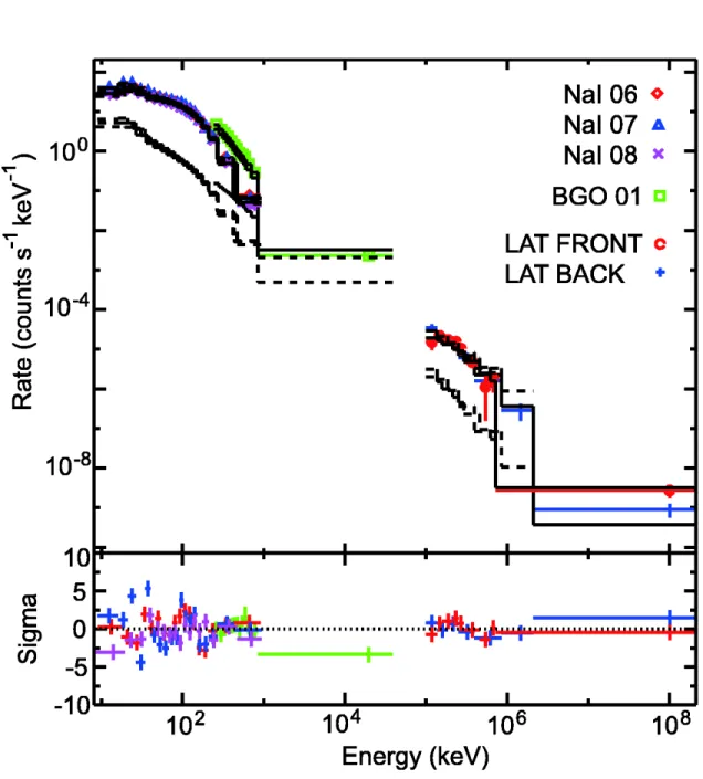
Fig. 4.— Joint spectral fitting of GBM and LAT data between T
0+ 3.3 s and T
0+ 21.6 s.
The top panel shows the count spectra and best-fit (Band+CUTPL) model (histograms).
The lower panel shows the residual of the spectral fitting.
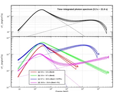
/s)2 (erg/cmνFν
10−7
10−6
Time−integrated photon spectrum (3.3 s − 21.6 s)
Energy (keV)
10 102 103 104 105 106
/s)2 (erg/cmνFν
10−8
10−7
10−6
10−5
a
b c
d
[a]: 0.0 s − 3.3 s (Band) [b]: 3.3 s − 9.7 s (Band) [c]: 9.7 s − 10.5 s (Band + CUTPL) [d]: 10.5 s − 21.6 s (Band + PL)
Fig. 5.— Top: The best-fit (Band+CUTPL) model for the time-integrated data plotted as a νF
νspectrum. The two components are plotted separately as the dashed lines, and the sum is plotted as the heavy line. The ±1 σ error contours derived from the errors on the fit parameters are also shown. Bottom: The νF
νmodel spectra (and ±1 σ error contours) plotted for each of the time bins considered in the time-resolved spectroscopy.
0.0001 0.001 0.01 0.1 1
1 10 100 1000
-3
-2.5
-2
-1.5
-1
Flux (MeV/cm2/s) Photon Index
Time since T0 (s)
Flux Fiting results Photon index