Brine Formation and Mobilization in Submarine
Hydrothermal Systems: Insights from a Novel Multiphase Hydrothermal Flow Model in the System H
2O–NaCl
F. Vehling1,3 · J. Hasenclever2 · L. Rüpke1
Received: 8 October 2019 / Accepted: 22 October 2020 / Published online: 19 November 2020
© The Author(s) 2020
Abstract
Numerical models have become indispensable tools for investigating submarine hydrother- mal systems and for relating seafloor observations to physicochemical processes at depth.
Particularly useful are multiphase models that account for phase separation phenomena, so that model predictions can be compared to observed variations in vent fluid salinity. Yet, the numerics of multiphase flow remain a challenge. Here we present a novel hydrothermal flow model for the system H2O–NaCl able to resolve multiphase flow over the full range of pressure, temperature, and salinity variations that are relevant to submarine hydrothermal systems. The method is based on a 2-D finite volume scheme that uses a Newton–Raphson algorithm to couple the governing conservation equations and to treat the non-linearity of the fluid properties. The method uses pressure, specific fluid enthalpy, and bulk fluid salt content as primary variables, is not bounded to the Courant time step size, and allows for a direct control of how accurately mass and energy conservation is ensured. In a first applica- tion of this new model, we investigate brine formation and mobilization in hydrothermal systems driven by a transient basal temperature boundary condition—analogue to seawater circulation systems found at mid-ocean ridges. We find that basal heating results in the rapid formation of a stable brine layer that thermally insulates the driving heat source.
While this brine layer is stable under steady-state conditions, it can be mobilized as a con- sequence of variations in heat input leading to brine entrainment and the venting of highly saline fluids.
Keywords Submarine hydrothermal systems · Numerical modeling · Phase separation · Brine layer · Mid-ocean ridges
* F. Vehling fvehling@geomar.de
1 GEOMAR Helmholtz Centre for Ocean Research Kiel, Wischhofstr. 1-3, 24148 Kiel, Germany
2 Institute of Geophysics, CEN, Hamburg University, Hamburg, Germany
3 Present Address: Institute of Geoscience, Kiel University, Kiel, Germany
1 Introduction
Hydrothermal venting at the ocean floor is a key mechanism of biogeochemical exchange between the solid earth and the global ocean. Fluid circulation through the young ocean floor sustains unique ecosystems (Boetius 2005), mobilizes metals from the crust to the ocean floor to form volcanogenic massive sulfide deposits (Hannington et al. 2011), and is a source of trace elements and isotopes that are now thought to play an important role in global scale biogeochemical ocean cycles (German et al. 2016). Much has been learned about these systems and their role in the Earth System from direct seafloor observations, water column measurements, ocean drilling, and geophysical imaging (Fornari et al. 2012;
German and Seyfried 2014; Humphris et al. 1995). Yet, the inner workings of submarine hydrothermal system remain inaccessible to direct observations. Instead, the sub-seafloor hydro-geochemical regime needs to be indirectly inferred. Investigating systematic pat- tern in vent fluid chemistry and their spatial as well as temporal variations is one powerful approach (e.g., Butterfield and Massoth 1994; Mottl et al. 2011; Shanks 2001; Von Damm 2004). The chemistry of hundreds of vent fluid samples taken from hydrothermal systems located in diverse geological settings including fast spreading and slow spreading ridges as well as back-arc spreading centers has been published. The resulting dataset shows a spectacular diversity and complexity of vent fluid chemistry, yet some first-order features and trends are robust and clear. For example, vent fluid salinity often deviates from the seawater value pointing to phase separation and segregation phenomena at depth. When seawater is heated and intersects the two-phase boundary, it splits into a low salinity vapor and a higher salinity brine phase (Bischoff and Rosenbauer 1984; Driesner and Heinrich 2007). Segregation of these phases can result in the venting of fluids that have a higher or lower salinity than seawater. Observed vent fluid salinities vary between 5 and 200% of the seawater value (3.2 wt% NaCl). These salinity variations are particularly interesting in the context of metal mobilization and transport. Most metals, including iron (Fe), are chloro- complexing and tend to travel with the more saline fluid phase, implying that phase separa- tion has a first-order effect on vent fluid chemistry (Butterfield et al. 1997; Jr. Seyfried et al.
1991; Von Damm 2004). Figure 1 illustrates this for a selection of vent fluid samples from the East Pacific Rise (EPR) and some selected slow spreading mid-ocean ridges.
Tracing salt within submarine hydrothermal systems is therefore a useful way of inves- tigating metal transport within the oceanic crust and toward the seafloor. Yet, relating changes in vent fluid chemistry to hydrothermal processes at depth remains a challenge and requires numerical multiphase transport models as well as a reliable equation of state (EOS) that can establish links between hydrothermal flow observations and physicochemi- cal processes at depth.
Some insights into brine formation and salt re-distribution within hydrothermal convec- tion cells can be gained from exploring the EOS of seawater (Driesner and Heinrich 2007).
Theoretical work on pure water (Jupp and Schultz 2000), later extended to salt water (Gei- ger 2005), has shown that the thermodynamic properties of (sea) water result in an upper temperature limit of approximately 400 °C in the upflow limb of submarine hydrothermal circulations cells (the exact value is a function of pressure and salinity). The critical point of seawater with 3.2 wt% NaCl is at 29.8 MPa and 407 °C. Consequently, boiling can occur at vent fields located at water depths shallower than ~ 3000 m. Such shallow boiling (and condensation) processes in combination with brine entrainment into the upflow zone are thought to be the reason for the high spatial and temporal variability in vent fluid salini- ties, which are, for example, observed at the East Pacific Rise vent field at 9°N located in
~ 2600 m water depth (Pester et al. 2014; Von Damm 2004; Von Damm et al. 1997). Boil- ing and entrainment processes are also likely to control vent fluid salinity at the ASHES vent field located in 1540 m water depth on the Juan de Fuca Ridge (JdFR), where chim- neys just tens of meters apart show salinities below and above seawater (Butterfield et al.
1990). These ideas were tested and confirmed with numerical multiphase models by Cou- mou et al. (2009), who showed how the entrainment of brines formed in the upflow zone of relatively shallow hydrothermal systems can result in rapid and large fluctuations in vent fluid salinity.
If a fluid of seawater salinity is intersecting the two-phase boundary at pressures higher than the critical pressure of seawater, small amounts of a highly saline brine phase are condensing from the fluid phase thereby depleting it in NaCl. Note that we do not use the terms “subcritical” and “supercritical” phase separation here, which are often found in mid-ocean ridge literature, because they refer to the misleading concept of a fixed salt con- tent. We rather follow Coumou et al. (2009) and refer to the physical processes of boiling and condensation. Brine condensation is likely to happen above the driving heat source of a circulation system. In most mid-ocean ridge settings, magmatic heat sources, e.g., the axial melt lens at fast spreading ridges or a gabbroic intrusion at slow spreading ridges, are located at hydrostatic pressures higher than the critical pressure of seawater and release their heat directly into the two-phase region. Within this region, the condensing dense brine phase will pool, while the less dense vapor phase will rise. This may result in a stable basal brine layer that insulates the heat source and through which heat transport is pre- dominantly conductive.
Based on mass flux estimates and measured vent salinities at Main Endeavor Field, Fon- taine and Wilcock (2006) estimated that a basal brine layer of ~ 100 m thickness should Fig. 1 Plot of chloride versus total iron for various vent fluids in mid-ocean ridge settings: East Pacific Rise (Shanks, 2001; Von Damm, 2000, 2004), TAG (Edmonds et al., 1996), Snakepit (Von Damm, 1990), Lucky Strike (Charlou et al., 2000; Von Damm et al., 1998), Rainbow (Douville et al., 2002), Longqi (Ji et al., 2017), and Edmond/Kairei (Gallant and Von Damm, 2006; Kumagai et al., 2008)
form within only 15 years. As this estimate was inconsistent with their calculated con- ductive heat balance, which required the brine layer to be thinner than 10 m to match the observed high heat flux, they argued that interfacial tension between fluid and solid phases will likely favor the segregation of vapor into the main fractures and brine into the smaller fissures. This would allow the vapor to flow efficiently through the system and to sustain large heat fluxes. Bischoff and Rosenbauer (1989) argued that double diffusion will break the stable stratification of the brine layer leading to internal convection, which mines the required heat from below. So far, the viability of both explanations remains questionable as neither has been tested in fluid dynamic simulations. A complementary explanation is lateral brine flow near the base of a circulation system. If brines move out of the two-phase region either by lateral migration or because heat supply is diminished, they would merge with the single-phase fluid flow above thus leading to the venting of highly saline fluids (Coumou et al. 2009). This process is likely to happen at the TAG hydrothermal mound on the Mid-Atlantic ridge, where stable brine venting (~ 125% of seawater salinity) has been documented to have occurred for more than a decade (Chiba et al. 2001). Long-term venting of brines is rare at intermediate to fast spreading ridges. Venting on the Northern Cleft segment of the JdFR is such an exception. Here repeated fluid sampling in the early 1990s documented persistent venting of high salinity fluids, which has been interpreted as interaction with a previously formed brine layer (Butterfield and Massoth 1994). At the Main Endeavor Field on the Juan de Fuca Ridge, vent fluid salinities have mostly been lower than seawater in the period 1984 to 2005 (Butterfield and Massoth 1994; Foustoukos et al. 2009; Lilley et al. 2003). Also at the East Pacific Rise at 9°50′N, low salinity vent- ing occurred for more than 13 years since 1991 (Von Damm 2004). This predominance of lower-than-seawater salinity venting at intermediate to fast spreading ridges raises again the question what the fate of the complementary brine phase is. It continues to be an unre- solved question whether brines are pooling at the base of circulation systems or brine vent- ing occurs diffusively or/and highly diluted.
It is in this context that we are here investigating brine formation and mobilization in submarine hydrothermal systems using a newly developed two-dimensional hydrother- mal modeling code. First, we present our numerical approach and explain our motives for developing a new code and how our approach differs from other existing simulators like CSMP++, MUFITS, TOUGH-NaCl and FISHES. Second, we show results of a suite of model calculations investigating a geometrically simple setup designed to approximate the conditions of a hydrothermal system at a mid-ocean spreading center with a basal heat source. For different pressure conditions, we study brine layer formation, its stability and effect on heat transfer as well as the conditions that result in the mobilization of the brine phase into the upflow zone.
2 Numerical Approach
2.1 Motivation for a New Thermohaline Code
Multiphase simulations of thermohaline flow in submarine hydrothermal systems continue to be numerically challenging and are still not routinely done. It requires an EOS that fully describes the fluid’s state and thermodynamic properties over sufficiently wide pressure (P), temperature (T), salinity (X) ranges, and a transport model able to handle multiphase
(2007) and Driesner (2007) provide complete and realistic correlation formulae for phase stability relations and fluid properties at temperatures from 0 to 1000 °C, pressures from 0 to 5000 bar, and compositions from 0 to 1 weight fraction NaCl. The provided EOS improves upon earlier works (Palliser and McKibbin 1998a, b, c) in the correlation for- mulae in that the complete fluid state can be calculated as a function of PTX including a comprehensive set of thermodynamic properties. The CSMP++ porous media simulator (Geiger et al. 2006a, b; Weis et al. 2014) uses this EOS and has been used for subma- rine hydrothermal systems (Coumou et al. 2009; Gruen et al. 2012, 2014) and geothermal sites (Scott et al. 2016, 2017; Weis et al. 2012). Other existing simulators include NaCl- TOUGH2 (Kissling 2005b), which uses different correlation formulae (Palliser and McK- ibbin 1998a, b, c) and is an enhancement of TOUGH2 (Kipp Jr et al. 2008), which was originally developed for geothermal settings below 350 °C. Yet this code was only used once for modeling in a case study for the Taupo Volcanic Zone in New Zealand (Kissling 2005b). FISHES (for Fully Implicit Seafloor Hydrothermal Event Simulator) has been developed by Lewis and Lowell (2009), the thermodynamic properties are a synthesis of data and extrapolations from various studies (Anderko and Pitzer 1993; Archer 1992; Pal- liser and McKibbin 1998a, b, c; Tanger and Pitzer 1989), and it is appropriate/adequate for modeling two-phase problems at mid-ocean ridges (Choi and Lowell 2015; Han et al.
2013; Singh et al. 2013). Most recently, the reservoir simulator MUFITS has been adapted to resolve multiphase hydrothermal flow using the EOS by Driesner and Heinrich (2007) and was used to simulate brine formation in a volcanic setting (Afanasyev et al. 2018).
According to publications, the well-documented CSMP++ simulator appears to be the most frequently used code. Interestingly, the employed sequential method of solving the governing equation is different to the typically used coupled approaches implemented in other hydrothermal and geothermal simulators. MUFITS, TOUGH2, HYDROTHERM and FEHM all use a coupled numerical approach, where mass and energy conservation equations are solved simultaneously using an iterative scheme, which is often the New- ton–Raphson method. It remains a question of active research to assess to strengths and limitations of sequential versus coupled approaches in terms of efficiency, stability, and accuracy. The reader can find further discussion on this in Ingebritsen et al. (2010), Vehling et al. (2018).
Coupled approaches should be better equipped for handling the strong non-linearities in the governing conservation equations and their strong couplings—and should theoretically be more efficient by allowing for larger time steps. In practice, the case is far from clear.
For example, resolving the sharp phase boundaries and associated jumps in coefficients that occur over the relevant PTX ranges in the H2O–NaCl system is a challenge in coupled approaches. Here the choice of the primary variables that define the thermodynamic state has to be done carefully. For the system H2O–NaCl, correlation formulae are a function of pressure, temperature, and composition, but the energetic state is not always resolved.
For example, saturations in the three-phase region where vapor, liquid, and halite coexist and for the pure water two-phase region cannot be calculated in PTX space (Figs. 2, 3).
One possible solution is primary variable switching (Class et al. 2002; Wu and Forsyth 2001). However, if a phase boundary is crossed multiple times, and each crossing triggers a primary variable switch and associated variable initialization, convergence can be poor.
In TOUGH-NaCl, this procedure leads to restrictions in the allowed phase state transitions (Kissling 2005b). For example, from single phase it is not allowed to have a direct transi- tion to the three-phase coexisting region.
Another option is to use a set of primary variables that always resolves the fluid state, e.g., pressure, specific enthalpy (H), and salinity. The downside is that the
existing EOSs for the system H2O–NaCl use PTX so that the thermodynamic state has to be determined with a costlier iterative scheme or with interpolations on look-up tables. In HYDROTHERM (Hayba and Ingebritsen 1994; Kipp Jr et al. 2008), this method has been shown to work well for the pure water two-phase region and also at difficult conditions around the critical point (22.06 MPa, 374.15 °C). Promising are also results obtained with MUFITS simulator which uses a PHX coupled scheme to resolve two-phase flow in the system H2O–NaCl (Afanasyev et al. 2018).
In summary, the equation of state for the system H2O–NaCl is reasonably well con- strained, but progress needs to be made in simulating multiphase transport. We see a large utility and potential for a hydrothermal simulator that uses the coupled approach with primary variables of pressure, spec. enthalpy, and composition. Recently, we have presented a coupled pressure/enthalpy scheme simulating pure water multiphase flow (Vehling et al. 2018). This method uses a higher-order time differencing scheme (theta- time differencing) that leads to higher accuracy, larger time step sizes, and a better convergence of the Newton–Raphson iteration scheme. We here extend this method to the system H2O–NaCl by adding an additional conservation equation and by translat- ing the EOS of (Driesner 2007; Driesner and Heinrich 2007) from PTX to PHX space.
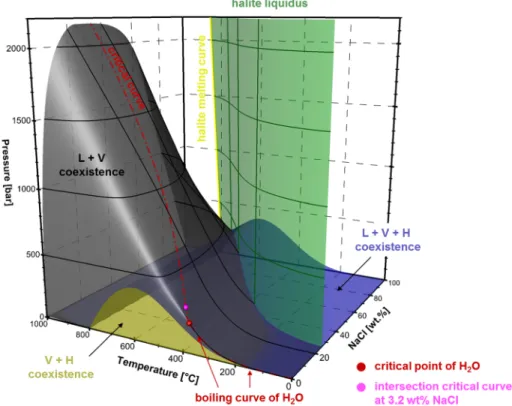
Fig. 2 Phase diagram of the system H2O-NaCl in temperature–pressure composition coordinates with iso- lines for pressure and composition on surfaces
2.2 Model Assumptions and Governing Equations
We use an extension of the two-phase flow model and numerical approach presented in (Vehling et al. 2018), which is a pure water two-phase numerical code. We make again the following model assumptions:
1. capillary pressure effects are neglected
2. rock and fluid are in local thermodynamic equilibrium
3. rock enthalpy is related to temperature by a constant specific heat
4. the inertia energy terms are orders of magnitude smaller and hence can be neglected 5. we fully account for pressure–volume work and viscous dissipation.
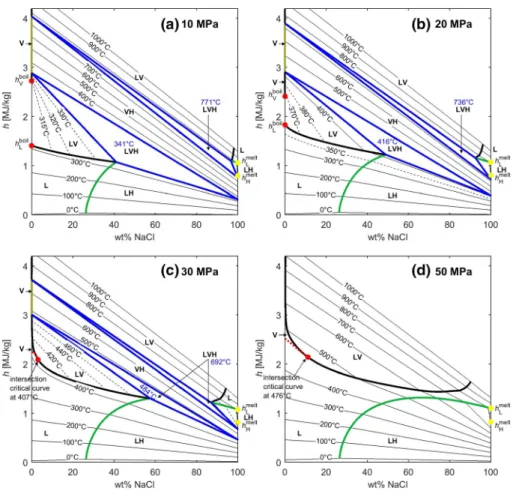
Fig. 3 Isobaric cross sections of bulk spec. enthalpy versus fluid salt content within the PHX phase rela- tion diagram. Colored bold lines show same phase region boundaries as shown in Fig. 2. Thin black lines are isotherms, crossing phase region boundaries. Dashed thin black lines are isotherms restricted to phase regions. a, b Red dots at the left border show spec enthalpy for boiling of pure water; boiling temperature is in a 311 °C and in b 366 °C. Temperatures of L + V + H regions are in blue. Yellow dots show spec.
enthalpy of melting halite hH and the corresponding melt hL. Molten halite is part of phase region L. Figure design has been adapted from Driesner (2013)
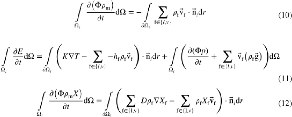
To describe the H2O–NaCl system, the conservation of mass of the combined H2O–NaCl fluid (Eq. 1) and the conservation of energy (Eq. 2) is completed by salt mass conservation (Eq. 3):
All variables are summarized in Table 1. Subscripts l, v, h stand for liquid, vapor, and halite phase and f is either liquid or vapor. The third term on the RHS of Eq. (2) describes viscous dissipation, and the fourth and fifth terms contain the part of the pressure–volume work that is not accounted for in the specific enthalpy. We summarize these terms into the following expression, which is then back-substituted into Eq. (2):
The fluid velocity trough a porous medium is described by Darcy’s law, where halite is treated as immobile phase, which is absent in advection terms.
The mean density ρm, mean specific enthalpy h, and mean salt mass fraction X are defined as follows, using Xh = 1:
where by phase volumetric saturations adding themselves to one:
𝜕( (1) Φ𝜌m)
𝜕t = −∇⋅ (∑
f∈{l,v}
𝜌fv⃗f )
(2)
𝜕E
𝜕t = 𝜕
𝜕t (Φ𝜌mh)
+𝜌rcpr𝜕(T(1− Φ))
𝜕t
= ∇⋅K∇T− ∇⋅ (∑
f∈{l,v}
hf𝜌f⃗vf )
+ ∑
f∈{l,v}
𝜂f
kkrfv⃗2f +𝜕(pΦ)
𝜕t + ∑
f∈{l,v}
v⃗f∇p
𝜕(Φ𝜌mX) (3)
𝜕t = ∇⋅ (
− ∑
f∈{l,v,}
𝜌fXfv⃗f )
+ ∇⋅ (∑
f∈{l,v}
D𝜌f∇Xf )
𝜕(Φp) (4)
𝜕t + ∑
f={l,v}
⃗vf( 𝜌f⃗g)
= − ∑
f={l,v}
⃗vf(
∇p−𝜌f⃗g) +
(𝜕(Φp)
𝜕t + ∑
f={l,v}
⃗vf∇p )
(5)
⃗vf= −kkrf 𝜂f
(∇p−𝜌f⃗g)
(6) 𝜌m=Sl𝜌l+Sv𝜌v+Sh𝜌h
(7) h= Sl𝜌lhl+Sv𝜌vhv+Sh𝜌hhh
𝜌m
(8) X=Sl𝜌lXl+Sv𝜌vXv+Sh𝜌hXh
𝜌m
(9) Sl+Sv+Sh=1
2.3 Equation of State in the System H2O–NaCl
We implemented the equation of state in the system H2O–NaCl published by Driesner (2007), Driesner and Heinrich (2007), which is formulated for the pressure–temperature composition space (Fig. 2). In total, we find seven phase states. The black surface sepa- rates the single-phase region from the liquid + vapor (L + V) coexisting region. The red line (critical curve) following the crest of this surface indicates whether a single-phase fluid enters the two-phase region as vapor-like or liquid-like fluid. At pressures below
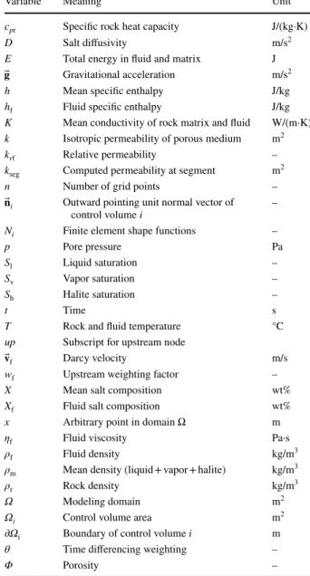
Table 1 Variables Variable Meaning Unit
cpr Specific rock heat capacity J/(kg·K)
D Salt diffusivity m/s2
E Total energy in fluid and matrix J
g⃗ Gravitational acceleration m/s2
h Mean specific enthalpy J/kg
hf Fluid specific enthalpy J/kg
K Mean conductivity of rock matrix and fluid W/(m·K) k Isotropic permeability of porous medium m2
krf Relative permeability –
kseg Computed permeability at segment m2
n Number of grid points –
n⃗i Outward pointing unit normal vector of
control volume i –
Ni Finite element shape functions –
p Pore pressure Pa
Sl Liquid saturation –
Sv Vapor saturation –
Sh Halite saturation –
t Time s
T Rock and fluid temperature °C
up Subscript for upstream node
⃗vf Darcy velocity m/s
wf Upstream weighting factor –
X Mean salt composition wt%
Xf Fluid salt composition wt%
x Arbitrary point in domain Ω m
ηf Fluid viscosity Pa·s
ρf Fluid density kg/m3
ρm Mean density (liquid + vapor + halite) kg/m3
ρr Rock density kg/m3
Ω Modeling domain m2
Ωi Control volume area m2
∂Ωi Boundary of control volume i m
θ Time differencing weighting –
Φ Porosity –
the critical point of pure water (pcrit = 22.06 MPa, 374.15 °C), the critical curve is iden- tical to the boiling curve of pure water. Here a single-phase fluid below the boiling tem- perature is always in a liquid state and would boil when heated to the two-phase bound- ary. At higher pressures, the critical curve moves to higher salt compositions, which implies that when a single-phase fluid with a salt content lower than the critical curve is heated until it hits the two-phase boundary, it would be a vapor-like fluid from which brine droplets are condensing.
Throughout this paper, we use the critical curve to distinguish between vapor- and liquid-like in the single-phase region at pressures higher than pcrit with vapor always having a lower density than a fluid on the critical curve for a given pressure. Therefore, a “vapor” is a fluid, which has a density below the density at the critical point of pure water (321.9 kg/m3), or a fluid having a higher temperature and a lower salt content than the critical curve at a given pressure.
The green surface marks the halite liquidus. In the liquid + halite (L + H) coexist- ing region, halite saturation increases linearly with increasing salt content, when tem- perature stays constant. The liquid, vapor, and halite coexisting surface (blue) forms the lower pressure boundary of the L + V region and the upper boundary of the V + H coexisting region. The dark yellow surface separates at low salinities the vapor region (single phase) from the V + H coexisting region.
We use a bisection method for the mapping between PTX and pressure, spec.
enthalpy, and composition space (PHX). Special care must be taken in regions where the fluid state is not uniquely described in PTX space, which is the three-phase, pure water boiling, and halite melting regions. Within those regions, we make use of the con- stant temperature constraint for a given pressure, which allows solving directly for the unknown saturations. Figure 3 shows HX-slices for different pressures illustrating how the fluid state is uniquely described in PHX space. Pure water boiling below the criti- cal pressure occurs at X = 0 between the specific enthalpies of vapor and liquid (Fig. 3a, b). If boiling occurs in the presence of salt (L + V region), the spec. enthalpies (and salt contents) of the vapor and liquid phases at a given temperature within the L + V region can be read off at the intersection of the respective isotherm with the phase region boundaries (bold lines). Note how the vapor phase can carry several wt% NaCl within the lower temperature range of the L + V region at higher pressures (Fig. 3c, d). At pres- sures lower than 39.015 MPa, the isothermal L + V + H coexisting field appears twice and the spec. enthalpies of each phase can be read off at the triangle corners (Fig. 3a, b, c). Within each (isothermal) lower temperature L + V + H region, an increase in bulk specific enthalpy results in the separation of liquid into vapor and halite, i.e., the liquid saturation decreases with halite and vapor saturations increasing. In the higher tempera- ture L + V + H regions, vapor and halite are progressively forming a very high salinity liquid (> 85 wt% NaCl) with increasing bulk enthalpy. Finally, isothermal halite melting is resolved with saturations of solid and liquid halite varying between the yellow dots at X = 1.
We have implemented the EOS in MATLAB but for performance reasons use pre- computed 3-D look-up tables for the transport models. For this purpose, we mesh differ- ent phase fields in 3-D PHX space using an unstructured mesh of tetrahedral elements.
In this way, we ensure that phase boundaries are well resolved and to not cross elements so that the interpolation scheme “knows” on which phase field it operates. Note that the EOS of Driesner and Heinrich (2007) does not include a parameterization of viscosity and we here use the one recently published by Klyukin et al. (2017).
2.4 Control Volume Method
As spatial discretization of the governing equations, we use a finite volume technique, in which a control volume (CV) is constructed around each node of an unstructured triangular finite element mesh (Fig. 4). This approach is equal to that used in Vehling et al. (2018) and has the advantage of being locally fluid mass, energy, and salt mass conserving. Mass and energy fluxes between two adjacent CVs are continuous when using temperature and pressure gradients obtained from corner nodes of the triangle elements. The same discre- tization is used in CSMP++ (Weis et al. 2014).
In the control finite volume method, fluxes are integrated over the boundary ∂Ωi of each CV. For each control volume Ωi, we obtain the integral formulations of Eqs. 1–3 by trans- forming the divergence of the flux terms into a line integral on ∂Ωi using the divergence theorem.
where n⃗i is the outward pointing unit normal vector field of the control volume boundary
∂Ωi. To calculate gradients across the segments, we use the spatial derivatives of standard linear finite element shape functions N.
∫ (10)
Ωi
𝜕( Φ𝜌m)
𝜕t dΩ = −∫
𝜕Ωi
∑
f∈{l,v}
𝜌fv⃗f⋅n⃗idr
(11)
∫
Ωi
𝜕E
𝜕tdΩ =∫
𝜕Ωi
(
K∇T− ∑
f∈{l,v}
−hf𝜌fv⃗f )
⋅n⃗idr+∫
Ωi
(𝜕(Φp)
𝜕t + ∑
f∈{l,v}
⃗vf( 𝜌f⃗g))
dΩ
∫ (12)
Ωi
𝜕( Φ𝜌mX)
𝜕t dΩ =∫
𝜕Ωi
(∑
f∈{l,v}
D𝜌f∇Xf− ∑
f∈{l,v}
𝜌fXf⃗vf )
⋅n⃗idr
Fig. 4 Construction of the control volumes Ωi from an unstructured finite element triangle mesh (black lines). The control volume boundary is composed of straight segments, and each element contains three segments
where x is an arbitrary point of Ω, j is the index of each node and its corresponding shape function, and n is the total number of nodes in the mesh.
2.5 Numerical Discretization in Time
For the numerical time discretization, we use a variable combination of forward Euler method and backward Euler method, the so-called theta (θ)-method:
Based on our efficiency study in Vehling et al. (2018), we favor the Galerkin Method with θ = 2/3.
2.6 Newton–Raphson Scheme
The main numerical difficulty in solving the above system of equations is the strong cou- pling between the mass and energy conservation equations and the strong non-linearity of the fluid properties. While the equation coupling is treated in our scheme by computing pressure, mean specific fluid enthalpy, and bulk salt content simultaneously during a single solve of the matrix equation, the non-linearity in fluid properties (and states) is resolved by NR iterations. For this purpose, we write the equations for each control volume (or associ- ated node) i in residual form:
(13)
∇p(x) = ∇
∑n j=1
Nj(x)pj=
∑n j=1
∇Nj(x)pj
(14)
∇T(x) = ∇
∑n j=1
Nj(x)Tj=
∑n j=1
∇Nj(x)Tj
(15)
∇X(x) = ∇
∑n j=1
Nj(x)Xj=
∑n j=1
∇Nj(x)Xj
𝜕u (16)
𝜕t =F(u,x,t)
ut+Δt−ut (17)
Δt =𝜃F(u,x,t)t+Δt+ (1−𝜃)F(u,x,t)t
Ri= −∫ (18)
𝜕Ωi
∑
f∈{l,v,s}
𝜌f⃗vf⋅n⃗idr−∫
Ωi
Φ𝜕( Φ𝜌m)
𝜕t dΩ
(19) Gi=∫
𝜕Ωi
(
K∇T− ∑
f∈{l,v}
hf𝜌fv⃗f )
⋅n⃗idr+∫
Ωi
(𝜕(Φp)
𝜕t + ∑
f∈{l,v}
⃗vf( 𝜌f⃗g)
−𝜕E
𝜕t )
dΩ
Then, we create a linear system of equations by applying the Newton–Raphson procedure for every residua Ri, Gi and Hi:
Here l + 1 refers to pressure, specific enthalpy, and salt composition after the next itera- tion step at time t + ∆t. Since each nodal residuum value depends only on the adjacent mesh nodes that are connected by the elements, all other derivatives are zero and the result- ing matrix is sparse. Since we use an implicit numerical method, these derivatives have to be calculated every time before solving the linear system of equations.
2.7 Calculation Of Darcy Velocity at Segments
When modelling phase separation phenomena, fluid properties between two neighboring grid nodes can vary over orders of magnitudes, especially when different phases exist on nodes or when large gradients in salt content occur. Therefore, the density at the segment, which is used for calculating fluid flow directions (
∇p−𝜌f⃗g)
, should account for salt con- tent at the upwind node and also for the temperature gradient. Therefore, we calculate a density for each phase and for the nodes on both sides of the segment:
We use ρf1,seg for calculating fluid fluxes if node 1 is the upwind node and ρf2,seg if node 2 is the upwind node.
Often a vapor phase is flowing into a colder control volume without a vapor phase so that no vapor density can be calculated there. For avoiding extreme vapor velocities flow- ing into cold CV at pressure conditions below 22.7 MPa, we use the following equation for calculating the density of a vapor phase at a segment.
(20) Hi=∫
𝜕Ωi
( ∑
f∈{l,v}
D𝜌f∇Xf− ∑
f∈{l,v}
𝜌fXfv⃗f )
⋅n⃗idr−∫
Ωi
𝜕( Φ𝜌mX)
𝜕t dΩ
(21)
∑n j
𝜕Ri
𝜕pj (
pl+1j −plj )
+
∑n j
𝜕Ri
𝜕hj (
hl+1j −hlj )
+
∑n j
𝜕Ri
𝜕Xj (
Xjl+1−Xjl )
= −Rli
(22)
∑n j
𝜕Gi
𝜕pj (
pl+1j −plj )
+
∑n j
𝜕Gi
𝜕hj (
hl+1j −hlj )
+
∑n j
𝜕Gi
𝜕Xj (
Xjl+1−Xlj )
= −Gli
(23)
∑n j
𝜕Hi
𝜕pj (
pl+1j −plj )
+
∑n j
𝜕Hi
𝜕hj (
hl+1j −hlj )
+
∑n j
𝜕Hi
𝜕Xj (
Xl+1j −Xlj )
= −Hil
(24) 𝜌f1,seg=0.5𝜌f1+0.5𝜌f(
p2,T2,X1)
(25) 𝜌f2,seg=0.5𝜌f2+0.5𝜌f(
p1,T1,X2)
(26) 𝜌v1,seg=0.5𝜌v1+0.5(
w𝜌(
p2,T2,Xcc)
+ (1−w)𝜌v,boil) w=1 ∀T2<Tboil−15◦C w=0 ∀T2>Tboil−5◦C w=(
Tboil−T2−5◦C)
∕10◦C otherwise
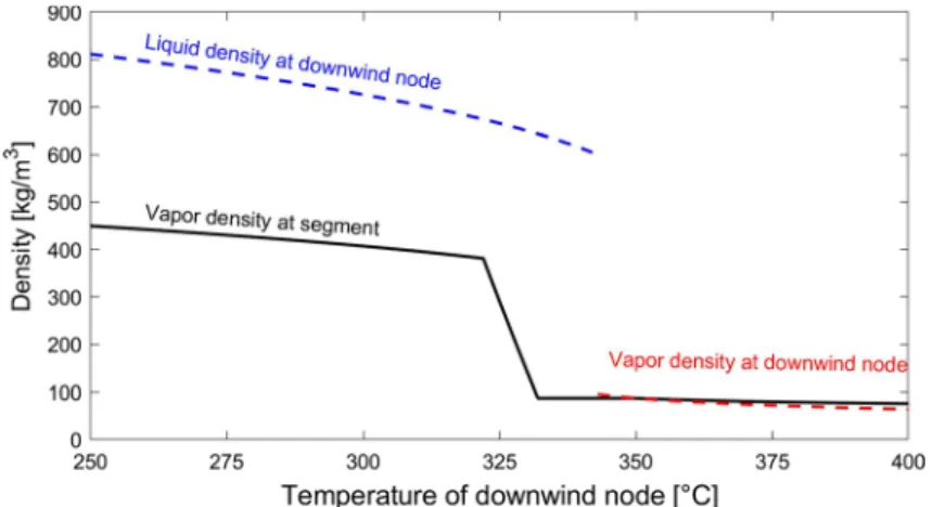
Note that boiling temperature Tboil and vapor density ρv,boil are a function of fluid pres- sure. Xcc is the salt content of a fluid at the critical curve (see Fig. 2) for a given pressure p2.This formulation takes into account the high difference between liquid and vapor densi- ties and leads to a better convergence of the Newton–Raphson scheme. In Fig. 5, we show a result of expression (26) for a pressure p2 of 15 MPa.
When the phase exists at the upstream side, we calculate fluxes over the segment using the upstream weighting method for fluid enthalpy, viscosity, relative permeability, and salt content. The density that is multiplied with the fluid velocity is also upwind weighted. We prefer full upwind weighting, because we want to avoid numerical oscillations in salt com- position. Additionally, when a phase does not exist at the downstream node, we save com- puting time by not creating synthetically downstream fluid properties.
2.8 Permeability and Relative Phase Permeability
When halite precipitates and fills up the pore space, rock permeability decreases. We have implemented the following function for the reduced permeability ki, which is also used in TOUGH2 (Pruess et al. 2012):
We computed permeability at segments using a logarithmic average, as it can vary over orders of magnitudes:
When permeability gets very low due to a high halite saturation, convergence of the Newton–Raphson scheme can become slow, especially for finding a good pressure solution for mass conservation. Therefore, we define a halite saturation threshold Sh max, and if it is exceeded, we set the permeability kseg to zero for all segments around this point. We then stop (27) ki=k(1−Sh)2
(28) kseg=exp
(ln( ki,up)
+ln( ki,do) 2
)
Fig. 5 Vapor density at the segment as a function of downwind node temperature T2 at a pressure p2 of 15 MPa using expression (26). The upwind node has a temperature of T = 350 °C, salt content of
solving for mass and salt mass conservation at theses nodes, but still solve for energy conser- vation by heat conduction. In the presented examples, Sh max is set to 0.95. This value is lower than required for numerical stability, but it is a reasonable assumption for submarine hydro- thermal systems that permeability drops to very low values at such high halite saturations.
When calculating relative permeability for liquid and vapor phase (krl and krv, resp.), we implemented a function in which the relative permeability is not additionally reduced by halite precipitation, because this is already accounted for in rock permeability (Eq. 27).
Therefore, relative liquid permeability is a linear function from 0 to 1, when Sl/(
1−Sh) exceeds the residual liquid saturation Srl:
2.9 Calculating Fluid (Salt) Mass and Energy in Control Volume
When modelling phase separation phenomena, salt composition varies over orders of mag- nitudes between adjacent nodes. For calculating the salt mass stored in a CV, we only use fluid properties of the node associated with the CV. Using the area of the CV, we compute fluid (salt) mass and energy as follows:
2.9.1 Convergence Criterion and Error Tracking
It is a challenging task to find good convergence criteria for the NR approach, when fluid properties and time step size vary over order of magnitudes. For the mass and salt mass conservation, we calculate an error of mass per square meter pore space over the time step
∆t in a CV of size Ωi:
As density and salt content could become very small, we need a second criterion, where we normalize the error by density or, respectively, density and composition:
krl= Sl/( (29) 1−Sh)
−Srl 1−Srl ∀Sl/(
1−Sh)
>Srl krl=0∀Sl/(
1−Sh)≤Srl
(30) krv=Sv/(
1−Sh)
(31)
∫
Ωi
Φ𝜌mdΩ = Φi𝜌m,iΩi
(32)
∫
Ωi
(Φ𝜌mh+ (1− Φ)𝜌rcprT) dΩ =(
Φi𝜌m,ihi+ (1− Φi)𝜌rcprTi) Ωi
(33)
∫
Ωi
Φ𝜌mXdΩ = Φi𝜌m,iXiΩi
(34)
‖‖Ri‖
‖a∶= Δt ΩiΦiRi
[kg m2 ]
For energy conservation, we find that it is sufficient to work with an error displaying joule per square meter.
We use following magnitude of criteria:
To ensure strict mass, energy, and salt mass conservation, we save the residual errors Ri, Gi, and Hi and add them as source term for the next time step. Here we have to consider old and new time step sizes:
2.9.2 Model Implementation and Limitations
The implemented Newton–Raphson method shows slower convergence, when the resid- ual conserving functions Ri, Gi, and Hi have discontinuities, which can arise from CVs experiencing phase transitions or from discontinuities in the relative permeability func- tions. Additionally, convergence is reduced when derivatives of the residual functions with respect to primary variables of the same CV become relatively small or change sign. A combination of both problems occurs, for example, at the phase transition into the isother- mal L + V + H region for Gi (energy conservation). Here, performance losses have to be accepted for code stabilization and convergence is achieved by reducing time step size and updating primary variables by reduced increments of the NR corrections until convergence.
For performance reasons, we use pre-computed look-up tables on unstructured tetra- hedral meshes for all fluid properties and their derivatives. Over each tetrahedron, fluid properties vary linearly and derivatives have constant values. This simple discretization can potentially lead to convergence problems, and in some cases, it may well be better to use the original correlation functions to compute the derivatives. However, this is computation- ally costly as the correlation functions are in PTX formulations and iterative procedures are necessary to obtain them in PHX space.
Additionally, the correlation functions for vapor density and vapor enthalpy in Driesner (2007) show an unexpected “loop” very close to the critical point of water at very low salt content. The vapor densities show a peak of too high values and the vapor enthalpies a peak of too low values. As a preliminary workaround, we use a coarser mesh near this region in the PHX space, which effectively linearizes fluid properties over the width of a (35)
‖‖Ri‖
‖b∶= ‖
‖Ri‖
‖a 𝜌m,i
(36)
‖‖Hi‖
‖c∶= ‖
‖Hi‖
‖a 𝜌m,iXi
(37)
‖‖Gi‖
‖d= Δt ΩiGi
[ J m2
]
(38)
‖‖Ri‖
‖a∶=1kg m2‖
‖Hi‖
‖a∶= ‖
‖Ri‖
‖1 3 ‖
‖Ri‖
‖b∶=0.01‖
‖Hi‖
‖c∶=0.01‖
‖Gi‖
‖d∶=105 J m2
(39) Ri,source=Roldi Δtold
Δt Gi,source=Goldi Δtold
Δt Hi,source=HioldΔtold Δt
We have implemented the entire multiphase model in MATLAB building upon the highly efficient MILAMIN and MUTILS tools (Dabrowski et al. 2008). An alternative would have been to implement the scheme using one of the existing FV libraries and/or transport models such as PFLOTRAN (Hammond et al. 2014), OpenFOAM (Weller et al. 1998), or DUNE/
pdelab (Bastian et al. 2010). We had opted for MATLAB because it provided us with the most flexibility and low-level control with regard to numerical implementation details. We hope that the presented details, especially on upwinding and phase weighting, will help with future 3D work on coupled multiphase hydrothermal flow models that may again be based on MAT- LAB or established FV libraries.
We tested our implementation against benchmarks and published results obtained by other codes. The respective benchmarks for pure water flow under single- and two-phase condi- tions have been presented in Vehling et al. (2018). Benchmarking of the saltwater case is less straightforward as the results strongly depended on the implemented EOS, which is unfortu- nately different among various published numerical models. We nevertheless show results of test cases used in previously published studies in "Appendix."
3 Simulation Results 3.1 Model Setup
We explore brine formation and mobilization in a simplified setup that mimics the situation at intermediate to fast spreading ridges, where hydrothermal circulation is mainly driven by heat released from a cooling axial melt lens (AML). The depth of the AML varies between 1 and 3 km beneath the seafloor and depends on magma supply as well as spreading rate (Morgan and Chen 1993; Theissen-Krah et al. 2011). The hydrostatic fluid pressure on top of the AML can therefore vary over tens of MPa between different ridge systems. We have performed numerical simulations for two different top pressure boundary conditions, 35 MPa and 20 MPa, in a domain of 3 km width and 1 km high. The grid has in total 6200 nodes and a refinement at the bottom center of 10 m node distance.
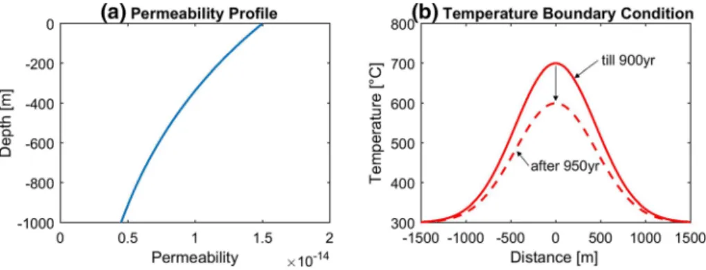
The sidewalls and the bottom domain boundaries are impermeable, and a fixed pressure boundary condition is used on top, which allows for free venting. Top inflow seawater temper- ature is 5 °C, and salt content is 3.2 wt%. The initial domain temperature is a linear function from top (5 °C) to the bottom (100 °C). At the bottom, we set a Gaussian-shaped temperature boundary condition with a maximum of 700 °C in the center and ~ 300 °C at the sides:
Here σ is set to 450 m and x is the lateral coordinate in the interval from − 1500 to 1500 m.
∆T is 400 °C. In addition, we assume the bottom row of control volumes to be impermeable so that heat transfer here occurs by conduction only. After 900 years, ∆T is linearly reduced to 300 °C over a time span of 50 years to explore the response of a basal brine layer to long-term variations in heat supply (Fig. 6). Rock permeability is a function of depth z:
where ktop = 1.5 × 10⁻¹⁴ m2 and b = 0.0012. We use a porosity of Φ = 0.03, a rock heat capacity of cpr = 880 J/(kg K), a rock thermal conductivity of K = 2 W/(m K), and a rock density of ρr = 2700 kg/m3. The residual saturation of the liquid phase Slr is set to 0.3.
(40) Tbot(x) =300◦C+ ΔT⋅exp
(
− x2 2𝜎2
)
(41) k(z) =ktop⋅exp(b⋅z)
3.2 Simulation 1: High Pressure Conditions (35 Mpa On Top) Lead To Stable Brine Layer Formation
The temperature boundary condition results in rapid heating within a central area of 1000 m width bringing the fluid into the two-phase regime. Figure 7a shows the situation after 300 years of heating: a basal brine phase containing up to 75 wt% NaCl has formed and the low salinity vapor phase has merged with single-phase flow above, forming a large low salinity region (1–1.5% NaCl). As the salt signal travels at pore velocity and hence faster than the temperature signal, venting of low salinity cold fluids occurs. Figures 7b and 8a illustrate the stable quasi-steady-state situation for this setup at t = 900 years. A stable basal brine layer has formed with little internal flow. Above it, and largely separated from it, single-phase high-temperature flow occurs at seawater salinity. In between, a thin two- phase region exists (Fig. 8a).
The central brine layer forms progressively from the bottom up. Brine saturations increase and two-phase flow occurs until the pore space is completely filled with brine.
“Gaps” in the brine layer that can occur due to changes in the convective pattern are filled up by lateral spreading of brines. Once the pore space is completely filled with brine, active phase separation moves higher up, where brine saturations then start to increase.
After 300 years, the brine layer has its largest extension with a maximum height of 90 m.
Due to this formation process, the brine salt content stays always very close to the liquid salt content side of the L + V coexisting surface (black surface in Fig. 2). No significant internal mixing of brines is observed, and single-phase flow above is separated from the stably stratified brine layer.
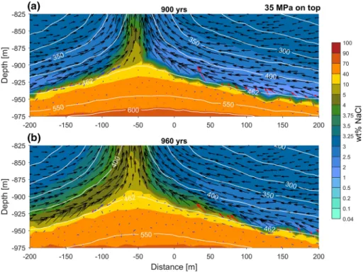
The top of the brine layer is equal to the 462 °C isotherm (Fig. 8). At this tempera- ture, vapor salinity at the L + V coexisting surface is equal to the seawater salt content of 3.2 wt% NaCl at 44 MPa. This implies that 462 °C is also the maximum temperature within the single-phase circulation system and that recharging fluids never experiences phase sep- aration once the system has reached this quasi-steady state. At this temperature, the brine phase has a salt content of 19 wt% NaCl and a density of 686 kg/m3, while the vapor phase has a density of 361 kg/m3. This factor ~ 2 density contrast is shown in Fig. 9 and leads to an interface, where vapor-like fluids are divided and kept separate from the brines below.
Figure 8 shows that the brine density increases with depth, which is a consequence of the increasing salt content with increasing pressure. Internal brine flow is therefore very low. At the top interface, brines are weakly affected by the overlying flow and are slowly
flowing toward the central upflow zone (Fig. 8a). Lighter brines can flow upwards leaving the brine layer, and heavier brines tend to flow very slowly downwards and then from the center toward the sides. The downward flowing brines become more saline and, as a result, very small amounts of vapor can form within the brine layer with saturation between 10–4 and 10–5.
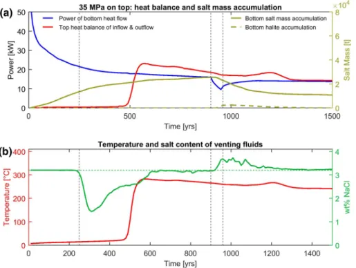
The brine layer itself acts as a thermal boundary layer. Over the first 40 years, the total conductive heat flux into the domain decreases rapidly due to decreasing temperature gra- dients at the bottom. After 40 years, heat flux is further decreasing in concert with the increasing amount of salt accumulated in the basal brine layer (Fig. 10a). The formed low salinity vapor phase mixes with single-phase flow above and after ~ 250 years low salin- ity and low-temperature venting occur. The temperature signal, being buffered by the host rock, travels slower, and vent temperature only starts to increase after 500 years. After the basal brine layer has reached its maximum extend, phase separation becomes limited as the single-phase circulation systems is effectively decoupled. Consequently, vent fluid salini- ties return to seawater values after approximately 600 years. When the temperature bound- ary condition is reduced after 900 years, the down flowing recharge fluids can merge with Fig. 7 Simulation results for a top pressure of 35 MPa. Color plots of total salt content in the pore space in wt% NaCl and temperature contours in °C
the brines at a lower temperature, and therefore, no formation of heavy brines and low salinity vapor occurs anymore (Fig. 8b). Instead, we find a higher mass flux of brines at the interface toward the center in between x-coordinate 60 m and 200 m. Also, deeper brines with high salinity are mobilized toward the center. These brines are further merging with Fig. 8 Scaled-up color plot of salt content and mass fluxes for a top pressure of 35 MPa. Black arrows dis- play liquids of X < 10 wt% NaCl. Blue arrows display liquids of X > 10 wt% NaCl. Red arrows display vapor (see definition for vapor in Sect. 2.3). Note that vapor can have up to 10 wt% NaCl at pressures of 45 MPa (see starting point of large red arrow in b) at 45 m with ~ 5 wt% NaCl). Arrow lengths have same scale fac- tor for all colors. White contour lines show isotherms in °C
Fig. 9 Fluid density and bulk density at L + V coexisting region
recharge fluids and a single-phase high salinity liquid of 5 to 10 wt% salt content forms that is sufficiently buoyant to rise. This merging process occurs over a very small tem- perature interval of 457–462 °C (T = 462 °C is temperature at critical curve at 44 MPa). At these temperatures, vapors have a relatively high salt content of 4 to 5 wt% (red arrows in Figs. 3c, d, 8b). Fluids of such high salinity do not reach the surface but rather mix with ambient seawater resulting in vent fluid salinities of only 3.5 wt%. Such mixing of ascend- ing fluids is further amplified by the increasing permeability toward the seafloor.
This mobilization of the brine phase in response to a decreasing bottom temperature results in a shrinking of the basal thermal boundary layer so that the 462 °C isotherm sta- bilizes at a deeper level. As a consequence, the bottom heat flow starts to increase again after 950 years and reaches nearly the old level after 1100 years (Fig. 10a) highlighting the importance of brine formation and mobilization in modulating heat input into the hydro- thermal system. We have repeated the numerical experiment with a reduced permeability ktop of 10–14 m2 and obtained the expected result of a 15-m-thicker basal brine layer. This confirms the arguments stated above that brine layer thickness is controlled by the balance between conductive heat flux from below and heat carried by the hydrothermal circulation system, which in turn is controlled by permeability.
Fig. 10 Simulation results for top pressure of 35 MPa. a Blue line: total power of conductive heat flow from bottom nodes into domain. Red line: Top power balance of inflow and outflow. Dark yellow line: bottom salt mass accumulation by considering halite and liquids with more than 10 wt% NaCl. Unit is tons of salt.
Dashed black lines show the points in time pictured in Fig. 7. b Red line: maximum outflow temperature.
Green line: salt content of fluid with maximal outflow temperature. After 900 years, the green line shows maximal salt content of outflow. Green dashed line show seawater salt content
3.3 Simulation 2: Mid‑Pressure Conditions (20 Mpa on Top) Lead to A Brine Layer on Top of a Halite Zone
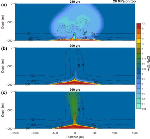
A reduction in the top pressure boundary condition results in a change in the stable phase assemblages and the dynamics of basal brine formation. In the mid-pressure set up, liq- uid–vapor separation is quickly followed by halite precipitation at the bottom. Here, at bottom pressures of 29 MPa, phase separation starts at temperatures of around 404 °C (Figs. 11, 12). The rising vapor phase has a very low salt content of only 0.1 wt% (at a tem- perature of 435°). Therefore, salt is rapidly accumulating at the bottom within the form- ing brine phase, whereas the rising vapor phase mixes with seawater resulting in a central upflow zone with salt contents of 0.3 to 1 wt% after 250 years, which is lower than in the high pressure case presented above (Fig. 11a). The basal brine phase has a salt con- tent of up to 55 wt% and, upon further heating to a temperature of 476.4 °C, enters three- phase conditions where liquid, vapor, and halite coexist (Fig. 3c). During further heating, the fluid leaves the three-phase region and the brine phase becomes separated into vapor and halite (upon entering the V + H field, Fig. 3c). Above the V + H region, brines that formed during phase separation within heated recharge fluids are slowly flowing (no visible
Fig. 11 Simulation results for a top pressure of 20 MPa. Color plots of total salt content in pore space in
blue arrows) into the V + H region where the salt of the brine is deposited as halite (see Fig. 12a; dark red color at 100 m to 200 m). This process results in a clogging of the pore space, which progressively blocks the pathways for heat mining vapors.
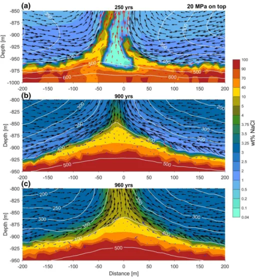
Figure 13 shows that the V + H region is continuously growing and halite saturation reach values > 90%. Also brine saturations in the overlying L + V region reach values of more than 95%. Compared to the high pressure simulation, the amount of salt accumu- lated in this basal boundary region is 3.5 times higher, and consequently, the salt content of venting fluids is substantially lower. After 900 years, a 20-m- to 30-m-thick brine layer has formed. This brine layer is less effectively separated from the overlying single-phase flow as it was in the high pressure experiment (Fig. 12b). The reason is that the layer is thinner and that the density contrast to the above single-phase fluid is smaller. At 400 °C, Fig. 12 Scaled-up color plot of total salt content and mass fluxes for a top pressure of 20 MPa. Black arrows display liquids of X < 10 wt% NaCl. Blue arrows display liquids of X > 10 wt% NaCl. Red arrows display vapor (see definition for vapor in Sect. 2.3). Arrow lengths have same scale factor for all colors.
White contour lines show isotherms in °C