Dissolution in a Waning Hydrothermal System
C. Schmidt1 , C. Hensen1 , K. Wallmann1, V. Liebetrau1, M. Tatzel2,3, S. L. Schurr4, S. Kutterolf1 , L. Haffert1, S. Geilert1 , C. Hübscher5 , E. Lebas6 , A. Heuser1 , M. Schmidt1 , H. Strauss4 , J. Vogl2 , and T. Hansteen1
1GEOMAR Helmholtz Centre for Ocean Research Kiel, Kiel, Germany,2Bundesanstalt für Materialforschung und‐ prüfung, Berlin, Germany,3Department of Earth and Planetary Sciences, University of California, Santa Cruz, CA, USA,
4Institut für Geologie und Paläontologie, Westfälische Wilhelms‐Universität Münster, Münster, Germany,5Institute of Geophysics, University of Hamburg, Hamburg, Germany,6Institute of Geophysics, University of Kiel, Kiel, Germany
Abstract
During R/VMeteorcruise 141/1, porefluids of near surface sediments were investigated tofind indications for hydrothermal activity in the Terceira Rift (TR), a hyperslow spreading center in the Central North Atlantic Ocean. To date, submarine hydrothermalfluid venting in the TR has only been reported for the D. João de Castro seamount, which presently seems to be inactive. Porefluids sampled close to a volcanic cone at 2,800‐m water depth show an anomalous composition with Mg, SO4, and total alkalinity concentrations significantly higher than seawater and a nearby reference core. The most straightforward way of interpreting these deviations is the dissolution of the hydrothermally formed mineral caminite (MgSO40.25 Mg (OH)20.2H2O). This interpretation is corroborated by a thorough investigation offluid isotope systems (δ26Mg, δ30Si, δ34S, δ44/42Ca, and87Sr/86Sr). Caminite is known from mineral assemblages with anhydrite and forms in hydrothermal recharge zones only under specific conditions such as highfluid temperatures and in altered oceanic crust, which are conditions generally met at the TR. We hypothesize that caminite was formed during hydrothermal activity and is now dissolving during the waning state of the hydrothermal system, so that caminite mineralization is shifted out of its stability zone. Ongoingfluid circulation through the basement is transporting the geochemical signal via slow advection toward the seafloor.Plain Language Summary
Hydrothermal vents are a common phenomenon in oceanic spreading centers worldwide. During Meteor cruise 141/1 we sampled sediments and extracted porefluids tofind thefirst indications for hydrothermal activity in the Terceira Rift. The results indicate that a hydrothermal vent close to a major volcanic cone formed in the past and seems to be in a waning state at present. Sampledfluids are enriched in total alkalinity, Mg and SO4. We found that the most straightforward explanation for this unusual finding is the dissolution of the hydrothermally formed mineral caminite, a magnesium‐sulfate‐hydroxide‐ hydrate. Caminite is a rare mineral but suggested to be abundant under specific conditions in hydrothermal recharge zones. We propose that caminite formed in the Terceira Rift is now dissolving as temperatures decline, andfluids enriched in Mg and SO4are transported along deep‐rooted faults to the seafloor.1. Introduction
Hydrothermal vents are common phenomena in slow‐to fast‐spreading centers worldwide (Beaulieu et al., 2013). Numerous authors provide a wealth of data on mineral assemblages andfluid chemistry of hydrother- mal systems and their recharge zones (e.g., Alt, 1995; Teagle et al., 1998). Hydrothermalfluid circulation is a driver for cooling of the Earth's crust and also plays a major role in geochemicalfluxes (Elderfield & Schultz, 1996). Generally, high‐temperature reactions are the reason that fluids become depleted in Mg and SO4
while Ca andfluid‐mobile elements like Li are enriched. Mg is quantitatively removed fromfluids by the for- mation of Mg‐rich smectite such as saponite (Alt & Honnorez, 1984). SO4in hydrothermal systems can undergo various reactions. At temperatures above 150 °C, SO4is typically removed by the precipitation of anhydrite (Alt et al., 1986; Teagle et al., 1998). However, SO4can also be reduced and precipitate as sulfide mineral (Alt, 1995). Ca is leached from the basement during albitization of plagioclase (Alt et al., 1986;
©2019. The Authors.
This is an open access article under the terms of the Creative Commons Attribution License, which permits use, distribution and reproduction in any medium, provided the original work is properly cited.
Key Points:
• Anomalously high Mg and SO4pore fluids in sediments of the Terceira Rift, Azores
• Indication for abundant caminite (Mg‐sulfate‐hydroxide‐hydrate) formation and dissolution in a hydrothermal recharge zone
• First indication for a deep submarine hydrothermal system in the slow‐spreading Terceira Rift
Supporting Information:
•Supporting Information S1
Correspondence to:
C. Schmidt, cschmidt@geomar.de
Citation:
Schmidt, C., Hensen, C., Wallmann, K., Liebetrau, V., Tatzel, M., Schurr, S. L., et al. (2019). Origin of High Mg and SO4
Fluids in Sediments of the Terceira Rift, Azores‐Indications for Caminite Dissolution in a Waning Hydrothermal System.Geochemistry, Geophysics, Geosystems,20. https://doi.org/10.1029/
2019GC008525
Received 25 JUN 2019 Accepted 5 NOV 2019
Accepted article online 11 NOV 2019
Humphris & Thompson, 1978). Levels of enrichment can vary, but concentrations of Ca influids can reach up to 80 mM (e.g., Butterfield et al., 1994). There are few studies focusing on mineral dissolution after cooling of hydrothermalfluid circulation (e.g., Gieskes et al., 2002; Gruen et al., 2014), leading to substantial changes influid compositions (e.g., enrichment in SO4and Ca due to anhydrite dissolutions, brine formation due to leaching of hydrothermally formed salts in the subsurface).
The Terceira Rift (TR) is a ~500‐km WNW‐ESE striking rift in the Central North Atlantic Ocean, marking the plate boundary between Nubia and Eurasia. The TR has been described as a hyperslow spreading center with a spreading rate of 4 mm a−1(Vogt & Jung, 2004). Cutting through the Azores Plateau, the TR com- prises four basins and passes through three volcanic islands of the Azores Archipelago (Figure 1). Albeit ongoing magmatic activity in this region, only nine onshore hydrothermal springs (Couto et al., 2015), and one offshore submarine vent, located at the D. João de Castro seamount (Figure 1), have been reported to date (Figure 1; Cardigos et al., 2005). However, during a previous Meteor expedition (M 128) in 2016 no signs of hydrothermal activity was detected at this location (Beier, 2016). Weiß et al. (2015) reported on 252 volcanic cones and sills in the eastern TR and theflanks of São Miguel, which possibly could host Figure 1.Overview Map: (a) Regional overview map modified from Weiß et al. (2015); TR: Terceira Rift; MAR: Mid‐ Atlantic Ridge; EAFZ: East Azores fracture zone; (b) detailed bathymetry map of core locations close to volcanic cone in the TR; (c) Multichannel seismic profile M79‐20 crossing TR.
hydrothermal systems. In the southern Hirondelle Basin major volcanic cones are connected to listric faults along the rift axis of the TR (Figure 1c), providing a potential pathway for the ascent of hydrothermalfluids to the seafloor. One of the major cones shows no sediment cover in the backscatter data (Weiß et al., 2015), which can be regarded as sign for recent magmatic activity. This volcanic cone provides presumably good preconditions to host a hydrothermal system. During R/VMeteorcruise M141/1 in September 2017 we sampled porefluids by gravity coring in the vicinity of the elongated volcanic cone to detect potential signs of ongoing hydrothermal activity in the TR.
2. Materials and Methods
2.1. Pore Fluid and Sediment Sampling
Two gravity cores (GCs) were retrieved during the cruise at 2,800‐m water depth. GC51 was taken on the fault close to the volcanic cone whereas GC50 was taken as a regional reference core (Figures 1b and 1c).
Both GCs had a length of 5.75 m and were equipped with a plastic liner. Right after retrieval on deck, the plastic liner was cut into 1‐m‐long segments and head space samples for hydrocarbon gas analyses were taken. The sampling interval was between 5 and 20 cm. Sediment samples were squeezed in a cold room with an argon gas squeezer. On average, squeezing took about 10 min. Gas pressure was usually up to 5 bar. The porefluid wasfiltered through 0.2‐μm cellulose Whatmannfilters.
2.2. Pore Fluid Analyses
On board analyses for total alkalinity (TA) were carried out using a METROHM titration unit 876 Dosimat plus. TA was determined by titration with 0.02 N HCl using a methyl red indicator. The solution was bubbled with argon to remove CO2gas released during the titration. On board analyses for NH4were carried out using a Hitachi U2800A spectrophotometer applying a calibration curve with eight standards covering the concentration range between 0 and 332.62μM. In our shore‐based laboratories at GEOMAR Helmholtz Center for Ocean Research, Kiel, cation concentrations (B, Ba, Ca, K, Li, Mg, Na, Si, and Sr) were determined using the Inductively Coupled Plasma Optical Emission Spectrometry (ICP‐OES, JY 170 Ultrace, Jobin Yvon). Anion concentrations (Cl, Br, and SO4) were analyzed using the Ion Chromatography (761 IC‐ Compact, Methrom). The IAPSO seawater standard was used to check the reproducibility and accuracy of the ICP‐OES and IC chemical analyses (supplemental data; Gieskes et al., 1991). The reproducibility is in general better than 1% relative standard deviation (RSD) for each element. Detailed description of the meth- ods can be found in for example, Hensen et al. (2007) and Scholz et al. (2009).
2.3. Solid Phase Analyses
Sediment samples from both cores were taken to determine their porosity, water content, chemical bulk ana- lyses, and petrological description (see Tables S3 and S4 in the supporting information). For the chemical bulk analyses, sediments were dried at 65 °C for 24 hr and homogenized. One hundred milligrams of each sample wasfilled into a Savillex vessel and treated with 2 cm3HF, 2 cm3HNO3, and 3 cm3HClO4 at 185 °C for 8 hr. Another 1 cm3of HNO3was added to smoke off the acid. The full method description is available in Scholz et al. (2016). After treatment with acids, sediment samples were measured by inductively coupled plasma optical emission spectroscopy (ICP‐OES) at GEOMAR, for concentrations of Al, Ca, Fe, K, Mg, Na, and Sr. The reproducibility is better than 1% RSD.
2.4. Smear Slides
Modal compositional data were obtained by counting at least 400 points in each of the 13 selected smear slides with a modified Gazzi‐Dickinson method based on Decker and Helmold (1985) and von Eynatten and Gaupp (1999) using a microstep point‐counting system and the Petroglide software without distinguish- ing into grain size fractions. The amount of 400 points was selected to derive a statistically significant estima- tion (e.g., Van der Plas & Tobi, 1965) of respective volume percentages of the components in the sediments.
We distinguish between 13 juvenile and nonjuvenile components. On the basis of common features four characteristic groups (total glass, total lithics, microfossils, and clay) were defined. Volume percentages of components or modal groups given in the text are normalized to 100%. Percentage raw data and calculated volume percentages of modal groups are listed in Tables S6 and S7 in the supporting information. Minerals like pyroxene, feldspar, amphibole, different types of pyroclasts, and sedimentary and volcanic lithics have not been subdivided in different species. Biogenic material has been subdivided into the main components
(nannofossils and foraminifers), and minor abundances have been summarized in “biogenic rest.”The reproducibility (2 times counting) was tested for two different samples and is better than 4% RSD regarding the modal groups. A detailed description can be found in the supporting information.
2.5. Si Isotopes
Porefluid samples were prepared for Si isotope measurements following the purification method of Georg et al. (2006). The samples were loaded onto 1‐ml precleaned cation‐exchange resin (Biorad AG50 W‐X8) and eluted with 2‐ml Milli‐Q water. Si isotopes were measured on the NuPlasma high‐resolution Multicollector‐Inductively Coupled Plasma Mass Spectrometer (HR MC‐ICPMS) in medium resolution mode using the Cetac Aridus II desolvator at GEOMAR. The Si concentration after sample purification equaled ~22μM, yielding Si recoveries of≥99% and a procedural blank below detection limit. The mea- surements were executed using the standard sample bracketing method to account for mass bias drifts of the instrument (Albarède et al., 2004). Si isotopes are given in the δ30Si notation, which represents the deviation of the sample30Si/28Si from that of the international Si standard NBS28. Long‐termδ30Si values of the reference materials Big Batch (−10.6 ± 0.2‰; 2 SD; n = 49), IRMM018 (−1.5 ± 0.2‰; n= 48), and Diatomite (+1.3 ± 0.2‰; 2 SD;n= 44) agree well with publishedδ30Si values in the literature (e.g., Reynolds et al., 2007). Additionally, an in‐house porefluid matrix standard has been measured, which yielded an averageδ30Si value of +1.3 ± 0.2‰(2 SD;n= 17). All samples were measured 2–3 times on different days and the resultingδ30Si values have uncertainties between 0.1 and 0.2‰(2 SD).
2.6. Sulfur Isotopes
Porefluids werefiltered (0.2‐μm pore sizefilter) and acidified (25% HCl) to a pH below 2. Subsequently, BaCl2solution (8.5%) was added to precipitate barium sulfate at 80 °C. The BaSO4precipitate was obtained viafiltration using a cellulose nitratefilter (0.45‐μm pore size). Forδ34S measurement 0.4‐mg barium sulfate mixed with 0.4‐to 0.8‐mg V2O5(catalyst) was placed into tin capsules. Theδ34S values were determined using an EA‐IRMS (Thermo Scientific Delta V advantage coupled with a Flash‐EA‐IsoLink‐CN Elemental Analyzer) at the Institute of Geology, Westfälische Wilhelms‐Universität of Münster, and are reported in the standard delta notation as per mil difference to the Vienna‐Canyon Diablo Troilite (V‐CDT) standards.
Analytical performance was monitored using international reference materials IAEA S‐1, S‐2, S‐3, and NBS 127 with an external reproducibility better than 0.6‰(2 SD). Forδ18OSO4analysis 0.2‐mg barium sulfate was placed in a silver capsule, andδ18OSO4was determined with a TC/EA‐IRMS (Thermo Scientific Delta V plus connected with a high‐temperature pyrolysis unit). Theδ18OSO4values are reported as per mil difference to the V‐SMOW standard. Measurement of replicate samples and reference materials (IAEA‐SO‐5, IAEA‐SO‐
6, and NBS 127) yielded an external reproducibility better than 1.0‰(2 SD).
2.7. Sr Isotopes
Sr isotope ratios (87Sr/86Sr) were measured by thermal ionization mass spectrometry (TIMS, TRITON, ThermoFisher Scientific) at the GEOMAR on aliquots of the original ICP‐OES pore water samples Table 1
Pore Fluid Data GC50 Depth
(cm)
NH4 (μM)
TA (meq/L)
B (mM)
Ca (mM)
Na (mM)
Mg (mM)
Sr (μM)
Si (mM)
Li (μM)
K (mM)
Cl (mM)
SO4 (mM)
Porosity (−)
12 11.40 2.99 0.464 10.68 483 53.8 87.2 0.19 28.1 10.7 559.7 28.6
23 39.85 3.06 0.458 10.88 484 54.4 88.7 0.21 27.2 10.7 566.8 29.3 0.65
48 89.19 3.27 0.465 10.63 487 54.8 88.1 0.25 27.2 10.8 572.8 29.4 0.62
60 113.00 3.20 0.440 10.08 481 53.3 85.7 0.25 24.9 10.7 566.9 28.4
71 123.80 3.20 0.445 9.81 480 52. 8 85.7 0.25 25.0 10.7 568.7 28.5
85 159.90 3.58 0.467 10.29 487 54.7 88.7 0.23 26.3 10.8 574.9 29.2 0.62
108 186.30 3.71 0.476 10.02 486 54.7 88.1 0.22 25.7 10.6 572.5 28.6 0.82
118 188.10 3.63 0.455 9.72 483 53.6 85.9 0.21 24.1 10.2 569.1 28.4
133 194.10 3.84 0.487 9.82 484 54.4 86.7 0.22 25.1 10.5 572.8 28.7 0.64
Note. Core Location: 37°58.345′N; 26°5.046′W; gray areas indicate ash and tephra layers.
(described above). According to the prior element concentration analyses (ICP‐OES) individual sample amounts equivalent to ~1,500 ng Sr (usually in the range of tens to hundreds ofμl pore water) were dried down in 2 ml of a 1 plus 2 mixture of 30% H2O2(supra pure) and 8 N HNO3(double distilled from per analyses quality). The separation of Sr followed a highly selective one step ion exchange chromatography using SrSpec resin (Eichrom) at whole procedure blanks of max. 60 pg. Before loading 100 to 200 ng Sr mixed with TaCl5activator on Re singlefilaments for TIMS measurements the Sr eluate was dried down in the H2O2/HNO3 mixture as described above. Repeated analyses of the standard NIST SRM 987 were used for performance monitoring and normalization of the measured87Sr/86Sr ratios applying a standard value of 0.710248 and reaching a reproducibility of ±0.000010 (2 SD,n= 10) throughout the study. The latter level of precision is representative for the individual sample results (see uncertainties given in Table 2 and Table 4). Furthermore, the IAPSO seawater standard a87Sr/86Sr ratio was determined on 0.709178 at ±0.000010 (2 SD,n= 4).
2.8. Ca Isotopes
Ca isotope measurements were performed on aliquots of the original pore water samples used for Sr isotope and element geochemistry ICP‐OES analyses, with the same pretreatment as described for Sr purification.
Calcium yields were >95% suggesting that Ca isotopes are not measurably fractionated by chemical purification (Morgan et al., 2011).
Prior to Ca isotope measurements samples were purified to remove matrix and interfering elements. We used a fully automated chromatographic purification system (prepFAST MC, ESI, Omaha, Nebraska, USA) following the method of Romaniello et al. (2015).
Calcium isotope measurements were performed on a MC‐ICPMS (Thermo Scientific Neptune, Thermo Fisher Scientific, Bremen, Germany) at the mass spectrometer facilities of GEOMAR. The mass spectrometer was set up to measurem/zof 42, 43, 43.5, and 44 simultaneously. In order to suppress interfering Ca‐and Ar‐hydrides (e.g.,40Ar1H2on42Ca) an APEX IR (ESI, Omaha, Nebraska, USA) sample introduction system was used. All measurements were performed in medium resolution (MR, m/Δm ~4,000) on the low mass side of the peaks (cf. Wieser et al., 2004).
Instrumental fractionation (mass bias) was corrected by applying the standard‐sample‐bracketing (SSB) approach. Interference correction for remaining sample Sr was done following the method of Morgan et al. (2011). Ca isotopes are given in theδ44/42Ca notation, which represents the deviation of the sample Table 2
Pore Fluid Data GC51 Depth
(cm)
NH4 (μM)
TA (meq/L)
B (mM)
Ca (mM)
Na (mM)
Mg (mM)
Sr (μM)
Si (mM)
Li (μM)
K (mM)
Cl (mM)
SO4 (mM)
Porosity (−)
16 64.57 4.05 0.448 10.66 485 55.7 101.8 0.21 29.5 10.3 560.6 29.5 0.59
30 88.09 4.67 0.452 10.41 481 55.5 109.6 0.22 28.9 9.8 564.7 29.4
40 114.50 4.94 0.473 10.79 490 57.4 116.9 0.25 31.9 10.5 571.8 30.3 0.61
50 140.10 5.27 0.481 10.60 488 57.4 118.9 0.26 32.9 10.4 571.8 30.5 0.61
55 144.50 5.57 0.469 10.36 486 56.7 121.1 0.24 31.4 9.9 567.3 29.8
63 179.30 5.60 0.480 10.78 490 58.3 128.1 0.23 33.6 10.8 571.8 30.6
82 221.00 6.42 0.501 10.65 491 58.6 135.1 0.26 35.6 10.2 571.5 30.8 0.62
92 6.58 0.485 10.46 489 58.6 136.0 0.22 36.7 10.3 575.9 30.8 0.60
107 324.00 7.99 0.516 10.98 490 58.9 142.8 0.35 37.6 10.1 573.1 30.9 0.66
122 290.30 7.58 0.523 10.85 492 59.5 147.9 0.24 38.7 10.1 561.7 30.6 0.62
127 268.50 7.52 0.509 10.70 488 58.2 149.3 0.23 37.2 9.6 567.6 30.6
134 277.90 8.03 0.531 10.88 491 59.3 151.1 0.23 40.2 9.9 573.3 31.2 0.65
142 293.00 8.33 0.532 10.99 489 59.1 153.7 0.23 41.0 9.9 572.3 30.8 0.64
153a 6.94 3.00 0.422 10.54 483 53.7 89.9 0.17 26.7 9.8 560.8 28.8
162a 40.13 3.99 0.473 10.84 485 55.7 100.6 0.20 29.7 10.5 564.8 29.7 0.59
Note. Core location: 37°58.049′N; 26°5.489′W; gray areas indicate ash and tephra layers.
aSamples were contaminated with seawater.
44Ca/42Ca from that of the international Ca standard NIST SRM 915a in per mil (‰). Long‐termδ44/42Ca of the reference materials NIST SRM 915b (0.35 ± 0.11‰, 2 SD,n= 13), NIST SRM 1486 (−0.50 ± 0.05‰, 2 SD, n= 131) and IAPSO (0.89 ± 0.06‰, 2 SD,n= 128) agree well with the literature values. A procedural blank for the Ca isotope work was determined and found to contribute less than 1% of the processed Ca.
2.9. Mg Isotopes
Mg was separated from matrix elements by cation chromatography using DOWEX AG 50 W‐X12 in polypro- pylene columns. Mg was eluted using HNO3(2 N). Splits (1 ml) before and after the Mg elution peak were screened for Mg as indicator for quantitative ion separation.
Mg isotope ratios were analyzed on a Neptune Plus MC‐ICP‐MS at Bundesanstalt für Materialforschung, Berlin. Samples and standards were introduced into a SIS spraychamber using a PFA microflow nebulizer with an uptake rate of 165μl/min. Measurements were done in medium resolution mode using a normal sample cone and a X‐skimmer cone. Procedural blanks are typically <7 ng Mg, of which <2 ng derived from the column procedure.
Measured Mg isotope ratios were normalized to the standard ERM‐AE 144 (Vogl et al., 2016) to compensate for mass bias drift (i.e., SSB). Samples and standard were diluted in HNO3(0.32 M) to≈0.75μg/ml Mg, where matching was better than 12%. Isotope ratios are reported in theδ‐notation, that is, as the deviation of a mea- sured isotope intensity ratio (I) with the high mass isotopesy=25Mg orz=26Mg over the low mass‐isotope
24Mg of a sample (smp) from that of a standard (std):
δMgy;z=24std ¼
Iðy;zMgÞ
Ið24MgÞ
smp
− Iðy;zMgÞ
Ið24MgÞ
std Iðy;zMgÞ
Ið24MgÞ
std
(1)
δvalues (abbreviated asδ25Mg andδ26Mg) were converted from the ERM‐AE144 reference frame into the DSM3 reference frame using equation (Vogl & Pritzkow, 2010) forδvalues obtained from the above equation in their basic form (no‰, ppm, or else). Whenδvalues in‰are to be used, they have to be divided by 1,000 before entering into the following equation.
δy;z=xE splð Þstd B¼δy;z=xE splð Þstd A−δy;z=xE std Bð Þstd Aþ δy;z=xE splð Þstd A·δy;z=xE std Bð Þstd A
(2) As quality control standards we have analyzed NASS‐6 (North Atlantic Seawater, NRC Canada) and the reference material ERM‐AE145. NASS‐6 yieldsδ25MgDSM3 =−0.37 ± 0.04‰andδ26MgDSM3=−0.74 ± 0.06‰(2 SD,n= 4), identical within 2 SD to the published values of NASS‐5 by Wombacher et al. (2009) withδ25MgDSM3=−0.43 ± 0.07‰(2 SD,n= 8) andδ26MgDSM3=−0.84 ± 0.16‰(2 SD,n= 4). Our mea- surements of ERM‐AE145 yieldδ25MgDSM3=−2.30 ± 0.05‰andδ26MgDSM3=−4.58 ± 0.08‰(2 SD,n= 3), identical within 2 SD with published values in Vogl et al. (2016) withδ25MgDSM3=−2.30‰andδ26MgDSM3
=−4.61‰.
The uncertainty ofδ‐values for the entire dissolution, separation and measurement procedure is estimated to
<0.1‰(2 SD).
2.10. Head Space Gas Analyses
Headspace gas composition of 20‐ml glass vials containing 3 cm3of sampled sediment and additional 6‐ml NaCl‐solution were prepared according to Sommer et al. (2009). The vials were stored upside down at room temperature until measurement by using gas chromatography at GEOMAR. One hundred microliters of headspace gas was injected into a Shimadzu gas chromatograph (GC‐2014), equipped withflame ionization detector and thermal conductivity detector (carrier gas: He 5.0; HayeSepTM Q 80/100 column, column length: 2 m; column diameter: 1/8"). The detection limits for CH4 and CO2 were 0.1 ppmV and 100 ppmV, respectively. Precision was about 4‰(2 SD).
Porewater concentrations of dissolved methane (mmol per liter porewater) were calculated by considering measured sediment porosity, molar volumes at laboratory pressure, and temperature. CO2values were used to determine pH values using the co2sys.xls program by Pelletier et al. (2005).
2.11. Endmember Calculations
Endmember (EM) calculations were performed for Mg, Ca, SO4, and Sr, assuming binary mixing of seawater and the theoreticalfluid EM. To calculatefluid EM we used element ratios versus elements for87Sr/86Sr versus Sr, Mg/Sr versus Mg, Mg/Ca; Ca, and Mg/SO4versus SO4. Seawater values were used as follows:
87Sr/86Sr = 0.709176, Sr = 90μM, SO4= 27.8 mM, Ca = 10 mM, and Mg = 53.2 mM. For thefluid EM, afixed value is required, which is typically Mg = 0 for hydrothermalfluids. Since this is not possible in this case we approximate EM concentrations by using afixed87Sr/86Sr ratio (see details in section 4.6). For each element ratio versus element concentration we calculated a mixing line using the following equation (here shown for the example87Sr/86Sr vs. Sr):
87Sr
86Srmix¼ fb½ Srb
87Sr
86Sr
bþð1−fbÞ½ Sra
87Sr
86Sr
a
fb½ Srbþð1−fbÞ½ Sra
(3)
A comprehensive list for all used element ratios with all data can be found in the supporting information.
2.12. Thermodynamic Model
The saturation state (SI) of caminite was calculated by comparing the ion activity product (IAP) of the solubility reaction to the corresponding thermodynamic equilibrium constant (K):
SI¼log IAP K
: (4)
The following stoichiometry was adopted for the dissolution reaction (Janecky & Seyfried, 1983):
MgSO40:25Mg OHð Þ20:2 H2Oþ0:8 Hþ↔1:25 Mg2þþSO4þH2O So that the equilibrium constant is defined as
Kcaminite¼ a1:25MgaSO4
10−pH ð Þ0:8aH2O
(5) wherearepresents the species activitities.
To test the evolution of the saturation index over a broad temperature and pressure range, three differ- ent thermodynamic equilibrium constants (valid for a SO4/Mg ratio of 0.625) were chosen from the work by Janecky and Seyfried (1983). In the lower temperature regionKcaminiteequals 5.3 and is valid for 25 °C and 1 bar. For data points near 200 °C Kcaminite is assumed to be −1.98 and is valid for 200 °C and 500 bar and the SI for 300 °C uses the value−5.59 for the equilibrium constant and is valid for 300 °C and 500 bar.
Species activities were calculated based on the molal concentration (m) and the activitiy coefficient (γ):
a¼γm (6)
The activity coefficients and the activity of water were computed based on the Pitzer model as described in and originally derived by Pitzer and Mayorga (1973). Interactions among the major sea ions were considered including Na, Mg, Ca, K, Cl, and SO4and their concentrations were set either to the bottom water values or the extrapolated endmember values. Respective Pitzer parameters were derived from internally consistent collections (Greenberg & Moller, 1989; Pabalan & Pitzer, 1987), which incorporate the effects of in pairing into their parameterization. It should be noted that the temperature range for the Pitzer data applied in the calculation of the species activities in most cases does not exceed 200 °C. Instead of extrapolating the
Pitzer parameters outside the stated temperature range, we use the parameterization of the upper temperature limit. For comparison, caminite SI is calculated for a range of pH values (7, 7.5, and 8). Also, while the equilibrium constants for elevated temperatures are valid only for 500 bar, we have also included the SI values that were calculated with activities for 1 bar to allow for a rough estimate of the pressure effect on the SI.
2.13. Transport Model
A simple 1‐D transport model including diffusion and advection was applied using Mathematica 11.3 (Wolfram Research, 2018). The model was solved for the solute species Mg, Ca, TA, and SO4. The general differential equation reads as follows:
∂ϕ·C
∂t ¼∂ ϕ·Ds·∂C∂x
∂x −∂ðϕ·v·CÞ
∂x (7)
wheretis the time (yr),xis the depth (cm),ϕis the porosity (unitless),Cis the concentration of solutes (mmol dm‐3), Ds is the diffusion coefficient in the sediments (cm2 yr‐1) corrected for tortuosity after (Boudreau, 1997), andvis thefluid velocity (cm yr‐1). The model did not include any reactions. Initial por- osity was set to 0.8, and porosity after compaction was set to 0.6 tofit the measured profile. Boundary con- ditions were defined for the sediment surface (0 cm) with ambient seawater concentrations (Mg = 54 mM, Ca = 10.2 mM, SO4= 28.7 mM, and TA = 2.7 meq/L), and for 300‐cm depth (Mg = 63 mM, Ca = 11.5 mM, SO4= 33 mM, and TA = 11 meq/L; note that the lower boundary conditions are not equal to the calculated EM). The model was run into steady state. The upwardflow velocity was determined byfitting the model to the measured pore water data.
2.14. Seismic Data
The reflection seismic data (Figure 1c) have been collected during RVMeteorexpedition M79/2 (Hübscher, 2012). Four so‐called GI‐Guns created the seismic signal and a 144‐channel, 600 m‐long seismic streamer, with a channel spacing of 4.2 m, recorded the data. Processing included band‐pass filtering, energy balancing, NMO‐correction, stacking, time‐migration, and fx‐deconvolution. For an overview of the marine seismic method, see Hübscher and Gohl (2014).
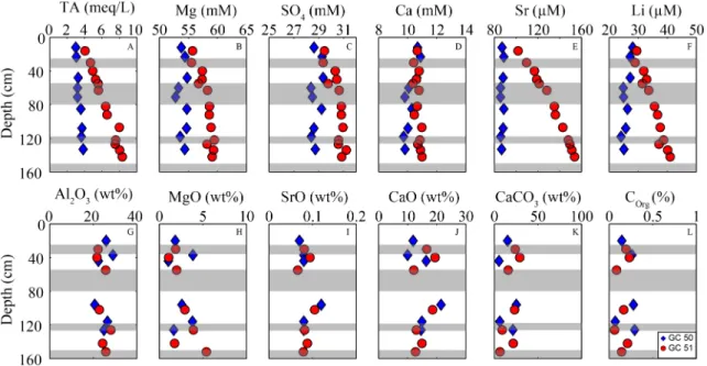
Figure 2.(a–f) Pore water profiles for Total Alkalinity, Mg, SO4, Ca, Sr, and Li; (g–l) depth profiles for solids of Al2O3, MgO, SrO, CaO, CaCO3, and COrg; Gray area indicates ash layers based on GC51.
3. Results
3.1. Pore Fluid Composition and Isotope Data
Porefluid depth profiles for TA, Mg, Ca, SO4, Li, and Sr are shown in Figures 2a–2f, and data are provided in Tables 1 (GC50) and 2 (GC51). The reference core GC50 shows a slightly elevated TA with 3.84 meq/L at 133 cm below seafloor (bsf). Ca is slightly decreasing from 10.86 at 12 cm bsf to 9.72 mM at 118 cm bsf. Sr is depleted in with respect to ambient bottom water (91μM), with a decrease to 86.73μM at 133 cm bsf. Mg, SO4, and Li do not show any deviations from seawater values. For GC51, TA increases downcore from seawater values of 2.35 meq/L to up to 8.33 meq/L at 142 cm bsf. Also Mg is increasing with depth to 59.46 mM at 122 cm bsf, and SO4increases from 27.8 to 31.21 mM at 134 cm bsf Ca remains almost constant over depth, with a slight increase up to 10.99 mM at 142 cm bsf with respect to seawater (10.2 mM). Sr in GC51 increases up to 150μM at 142 cm bsf. In addition to that Li is also increasing to 40μM in GC 51.
Isotope systematics of GC51 show a strong deviation from seawater for87Sr/86Sr andδ26Mg and only minor deviations forδ34S,δ44/42Ca, andδ30Si (Figure 4 and Table 3).87Sr/86Sr shows a decreasing trend from 0.7091 (present‐day seawater) to 0.7074 at 142 cm bsf.δ26MgGC51values of the sampledfluids show an increase inδ26Mg from−0.81‰(seawater) to−0.18‰at 142 cm bsf.δ34SGC51increases with depth from 21.9‰at 16 cm bsf to 24.7‰at 134 cm bsf.δ44/42CaGC51 does decrease slightly from 0.84‰at 50 cm bsf to 0.77‰at 142 cm bsf.δ30SiGC51does on the other side show no deviation from seawater values with depth. In contrast to GC 51 all isotopic ratios measured for GC50 do not show any or only minor (87Sr/86Sr andδ34S) deviations from present day seawater values (Figure 4 and Table 3).
3.2. Solid Phase
The sediments largely consist of nannofossil‐rich mud to mud‐rich nannofossil ooze with vari- able admixture of fresh volcanic, siliciclastic, and biogenic material. A detailed description of sediments and components can be found in the supporting information. Organic input to sedi- ments is low resulting in an average amount <0.3% of COrg. CaCO3proportion of the sediments is in average ~20%. The main composition of the sediments is rather constant over depth and does not show pronounced differences between the two coring locations (Figures 2g–2l). The Chemical Index of Alteration (CIA; Nesbitt & Young, 1982) is used as a measure to determine the degree of weathering of the sediments. The CIA is calculated as follows: CIA = Al2O3/ (Al2O3+ CaO*+ Na2O + K2O) × 100. CaO* is the Ca bound to silicates and is determined by subtracting Ca bound to carbonates (CaCO3= 8.33 * TIC) from total Ca. The average CIA for both cores is between 40% and 60% (details can be found in the supporting information data).
3.3. Head Space Gas
Head space gas analyses for CH4and CO2did not show any variations with depth (see support- ing information for data). CH4values stay at background values. The highest methane concen- tration was observed in GC50 at 166 cm bsf with 0.739μM. In addition to that, also fCO2values remain at background values with slightly elevated values for GC51. fCO2 values go up to 5,599 ppm in GC51. The calculated pH values from fCO2and TA concentrations are for both cores about 7.5.
4. Discussion
In the following, we will present a comprehensive analysis of potential processes that might explain the unusual geochemical pore fluid signature of GC51 with anomalously high TA, Mg, and SO4concentrations.
4.1. Near‐Surface Diagenetic Processes
Pore water profiles of enriched species display a slight exponential curvature within the upper- most ~50 cm (Figure 2). Generally, such type of profiles can either be the result of continuous reactive processes or be caused byfluid advection. Reactions typically include organic matter Table3 IsotopeResultsfor87 Sr/86 Sr,δ34 S,δ18 OSO4,δ26 Mg,δ30 Si,andδ44/42 CaforGC50andGC51 Depth(cm)87 Sr/86 Sr2SDnδ34 SSO4 [‰;V‐CDT]2SDnδ18 OSO4 [‰;V‐SMOW]2SDnδ26/24 Mg [‰;DSM3]2SDnδ30 Si [‰;NBS28]2SDnδ44/42 Ca [‰;SRM915A]2SDn GC50 230.7090610.0000073——————−0.800.0631.630.1520.880.074 1330.7088170.000010424.20.08215.90.462−0.750.0431.410.2320.860.084 GC51 16———21.90.10211.00.822———1.60.223——— 500.7080840.000013423.00.02214.00.972−0.390.0431.790.2230.840.084 820.7077520.0000104——————−0.300.0631.460.1830.810.054 134———24.70.05217.50.802————————— 1420.7074280.0000083——————−0.180.0531.220.0820.770.054
degradation, secondary redox reactions, weathering/alteration of rocks, and mineral dissolution reactions.
Our data suggest that the reactive influence in the shallow sediments is only minor: The TR in the Central North Atlantic Ocean receives only minor input of organic matter reflected by very low concentra- tions of TOC (<0.3 wt.%). Moreover, the increase in TA that results from organic matter degradation should also have been observed in GC50 where the increase is almost negligible. The increase in TA could also be explained by the anaerobic oxidation of methane (AOM) coupled to sulfate reduction. This would require a deep methane source, but neither indications for sulfate reduction (SO4 concentrations are elevated in GC51) nor methane enrichment were detected in GC51. We assume that some of the elevated TA in GC51 comes from minor organic matter degradation, but additional processes have to be considered.
Weathering/alteration of rocks or mineral dissolution processes could onfirst sight explain the curvature in the increasing profiles in GC51. Weathering of the volcaniclastic sediments can have an effect on thefluid composition, as minerals like Mg‐smectite and zeolites can be formed or elements can be released due to vol- canic glass dissolution (Schacht et al., 2008). However, visual analyses of the surface sediments by smear slides did not reveal indications for altered volcanic compounds or any secondary Mg or SO4bearing miner- als (e.g., being indicative for hydrothermal alteration). Furthermore, the sediments of the reference core GC50 are identical in composition and depth of stratigraphic layers compared to GC51 (Figures 2g–2l).
Intense weathering and formation of secondary minerals typically results in the loss of alkaline and alkaline earth metals, which is reflected in high values (>75%) of the CIA. CIA values for both cores do not show any evidence for pronounced alteration processes and no depth‐related trends.
4.2. Indications for Upward Fluid Flow
The lack of evidence for alteration processes in the near‐surface sediments suggests that the geochemical composition of thefluid is not the result of in situ processes but instead seems to be derived from deeper sources. The application of a simple numericalfluid transport model was carried out to test if the shape of the profiles (Figures 2a–2f) can be explained by an advectiveflux component. We tested two model scenarios (i) only diffusion and (ii) advection and diffusion (Figure 3). Indeed, a reasonably goodfit to the data could be obtained with afluid velocity of 0.5 cm yr‐1, emphasizing the need to include the advection process in the profile interpretation. With shallow diagenetic processes being only of minor importance, the hypothesis thatfluids are derived from a deeper source is supported.
4.3. Hydrothermal Signature
With respect to the location close to an active spreading center and recent magmatic activity in the area, we suspect that the observed pore water anomalies are related to hydrothermal activity. Many processes in hydrothermal systems do affect Mg and SO4concentrations offluids. Below, we analyze potential processes that might cause such anomalies and discuss their likeliness.
4.3.1. SO2‐Enriched Volatiles
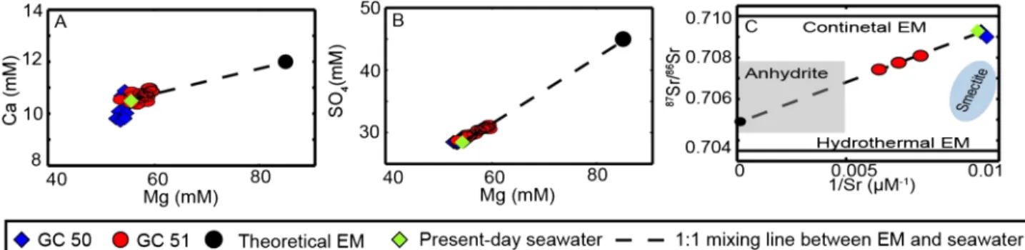
Hydrothermalfluids enriched in Mg and SO4have been reported from other regions, for example, the DESMOS caldera (Gamo et al., 1997; Seewald et al., 2015). In these cases, the excess SO4concentrations were explained by the discharge of SO2‐enriched magmatic volatiles and their subsequent disproportionation to SO4. Such highly acidicfluids can leach Mg‐rich silicate minerals from the host rock, resulting in increased Mg concentrations (Gamo et al., 1997). Sulfur of magmatic origin can be distinguished from seawater sulfur and other sources by itsδ34S signature. Fluids sampled at the DESMOS caldera show much lower values compared to seawater and, hence, are typical for a mantle sulfur source (δ34SMantle< 5‰; Seewald et al., 2015). In contrast,δ34SGC51values increase slightly and stay at levels above seawater (Figure 4a). A mantle origin of SO4via disproportionation from SO2we can rule out.
4.3.2. Anhydrite Dissolution
One of the most abundant minerals formed in hydrothermal systems is anhydrite. Hydrothermal anhydrite formation is a major sink for SO4, resulting in the removal of SO4fromfluids (Alt, 1995). The mineral phase forms at temperatures above 150 °C but is generally not present in old, altered oceanic crust as it dissolves at lower temperatures (Alt, 1995). Dissolution of anhydrite could therefore be a source for SO4to the porefluids (Gieskes et al., 2002).δ34S values of anhydrite are typically around or slightly above seawater (Alt, 1995), matching our observations in thefluids (Figure 4a). In contrast, Ca concentrations are not significantly ele- vated in GC51, albeit the fact that anhydrite dissolution releases equal amounts of Ca and SO4to the pore fluids. Moreover, an extensive dissolution of anhydrite should result in much stronger deviations of the
δ44/42CaGC51 = 0.77‰from δ44/42CaSeawater = 0.89‰(Figure 4b). Anhydrite has a shift of 0.5‰ from seawater to lower values (Amini et al., 2008). Thus, an additional sink for Ca, for example, calcium carbonate formation or ion exchange with clay minerals would be required or only a minor dissolution of anhydrite seems plausible here. Additionally, dissolution of anhydrite could explain the elevated Sr concentrations. Sr is an abundant trace element in hydrothermally formed anhydrite (Teagle et al., 1998).
However, anhydrite dissolution cannot explain the increased TA or Mg concentration.
4.3.3. Mg‐Rich Smectite
Mg‐rich smectite, such as saponite, is the major sink for Mg in hydrothermal systems (Alt et al., 1986). In contrast to anhydrite, saponite is present in aged oceanic crust and is not dissolving during cooling of hydro- thermal systems (Alt & Honnorez, 1984). Mg Smectite dissolution can be excluded as potential source for the Mg excess relative to seawater. Clay minerals do have a significant ion exchange capacity due to their large surface area. The main cations being exchanged are Mg, Ca, H, and Na (Wimpenny et al., 2014).
Accordingly, smectite could be a potential sink for Ca and source for Mg. The overallδ26Mg of Mg‐smectites is above 0‰(Figure 4c, Teng, 2017). Most of Mg is bound to the clay mineral lattice and only absorbed Mg in the interlayers can be exchanged. The exchangeable Mg of smectite is typically around −1.5‰δ26Mg (Wimpenny et al., 2014) and therefore lower than seawater values. Consequently, ion exchange should result in a decrease of theδ26Mg value in thefluid relative to theδ26Mg in seawater, which is opposite to theδ26Mg values in GC51. In contrast, the dissolution of Mg‐rich silicates by acidicfluids yieldsδ26Mg values between
−0.15‰and−0.25‰(Teng, 2017), identical with the porefluidδ26Mg.in GC51.
Silicon isotopes (δ30Si) can be used as an additionalfluid tracer, as different reservoirs are characterized by distinctδ30Si values. Mantlefluids have an averageδ30Si value of−0.3‰(De La Rocha et al., 2000). Also secondary clay mineral dissolution would enrich thefluid phase in light28Si, as clays show on average lowδ30Si values of−2.1‰ (De La Rocha et al., 2000; Ziegler et al., 2005; Opfergelt et al., 2010). The δ30Sivalues in GC51 range between +1.2‰and +1.8‰(Figure 4d) and thus overlap within error of the Si isotope value of the deep Atlantic water at 2,800 m water depth (averageδ30SiAtlantic= +1.6‰(Brzezinski
& Jones, 2015; De Souza et al., 2012), and the reference core GC50, which has an averageδ30Si value of +1.5‰(see Table 3). Consequently, dissolution of secondary Si‐rich minerals or mixing with mantlefluids can be excluded as well.
4.3.4. Low‐Temperature Weathering of Peridotite
Snow and Dick (1996) proposed that the weathering of peridotite at temperatures below 150 °C results in the pervasive loss of Mg of the basement. Slow‐spreading ridges are the typical environments were peridotites get exposed to the seafloor surface. Ligi et al. (2013) proposed that the increase in number of slow‐spreading ridges in the past 80 Ma have contributed to a shift in the global Mg cycle as enhanced weathering of peridotites could have occurred. However, up to date no Mg‐rich fluids have been found in slow‐ Figure 3.Transport model results for both scenarios: (i) diffusion (dashed line) and (ii) diffusion and advection (solid line) for (a) TA; (b) Mg; (c) Ca, and (d) SO4.
spreading environments. The hyperslow spreading TR could be suitable for the conditions defined for high Mg vents by Ligi et al. (2013). The crustal thickness of the basaltic Azores Plateau is about 14 km (Escartin et al., 2001), and exposure of mantle peridotite is unlikely here. In addition to that, no description of exposed peridotites is available for the TR. Nevertheless, if a deepfluid circulation could reach peridotites, low temperature weathering of peridotites results in the formation of Mg‐smectite, accompanied with a fractionation of Mg isotopes (Liu et al., 2017). According to the authorsfluids enriched in Mg affected by low‐temperature weathering result inδ26Mg values lower than seawater by−1.31‰, whileδ26Mg values in core GC51 are enriched with respect to seawater. Hence, we conclude that this process is not or at least not significantly affecting thefluid composition at GC51.
4.4. Dissolution of Caminite
None of the processes described above can satisfactorily explain the geochemical porefluid anomalies of high Mg, SO4, and TA concentrations observed in GC51. All of the above discussed processes only impact one of the three enriched species. A complex succession of these processes can also not satisfactorily explain thefluid geochemistry at GC51. We suggest therefore that we see here as of yet underestimated case where the dissolution of the hydrothermally formed mineral caminite may offer an explanation for the observed pore fluid deviations. Caminite is a magnesium‐sulfate‐hydroxide‐hydrate (MgSO4 0.25 Mg (OH)2
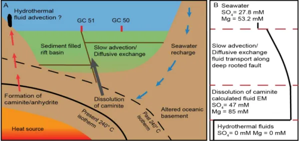
0.2H2O), which to date has been only found once in a natural environment. Haymon and Kastner (1986) reported caminite from a black smoker site on the East Pacific Rise 21°N, precipitating directly from heated seawater. Furthermore, this mineral has been synthesized under laboratory conditions (Janecky & Seyfried, 1983). Both studies indicate that highfluid temperatures of >240 °C are needed to form caminite. Although caminite can be regarded as a rare mineral, Haymon and Kastner (1986) proposed that it could be an abundant mineral in hydrothermal recharge zones where high temperatures are present in the system while Mg‐smectite formation is largely inhibited. The authors assumed that such a scenario is possible in hydro- thermal systems with little fresh basaltic glass present in the recharge zone. This implies that during a former hydrothermal alteration Mg‐smectite already formed and the reactivity of the basement is lower compared to young oceanic basement. The basement of the Azores Plateau has undergone intensive alteration (Beier et al., 2019); hence, there is the possibility that smectite formation has occurred before and no fresh basaltic glass is present at this location in the basement. Moreover, an enrichment of Li influids is indicative for elevatedfluid temperatures in the subsurface (e.g., Scholz et al., 2010). The Li concentrations in GC51 are slightly elevated compared to the reference core; we can therefore assume that highfluid temperatures are present in the subsurface in the TR.
Thus, the general conditions for the formation of caminite (as defined by Haymon & Kastner, 1986) are likely to be met in the TR. It has also been shown that caminite dissolves rapidly at temperatures <240 °C Figure 4.Depth profiles for isotopes and potential sources; the shaded area in (a) and (b) represents the estimated range ofδ26Mg andδ34S‐values of caminite.
(a)δ34SSeawater= 21‰;δ34SEvaporites= 19–25‰;δ34SMantle= 0–5‰(Alt, 1995); (b)δ26MgSeawater= 0.81‰,δ26MgCarbonate<−2‰, mantle =−0.4 to−0.2‰ (Teng, 2017);δ26Mgexchangeable of smectite=−1,5‰;δ26Mgstructurally bound in smectite= 0–0.5‰(Wimpenny et al., 2014);δ26MgLow‐T alterationfluids=
−1.31‰(Liu et al., 2017); (c)δ30SiSeawater= +1.6‰,δ30SiMantle=−0.3‰,δ30SiSecondary Mineral=−2.1‰; (d)δ44/42CaSeawater= 0.9‰,δ44/42CaAnhydrite= 0.3‰, the shaded area in (a) and (c) indicates the presumed isotopic composition for caminite.
(Haymon & Kastner, 1986). Decreasing temperatures after hydrothermal activity could result in the dissolu- tion of previously formed caminite increasing the Mg and SO4concentrations in the ambientfluids. This is also in line with the additional increased TA in GC51 compared to GC50 due to the release of (OH)‐through the dissolution of caminite.
According to Janecky and Seyfried (1983), caminite is present in two modifications with different SO4/Mg ratios. The authors describe one modification with SO4/Mg = 0.625, which is the more stable phase at tem- peratures above 300 °C and pressures below 500 bars, and caminite with SO4/Mg = 0.7, which is more stable at temperatures below 300 °C and 500 bars. In addition the SO4/(OH)−ratio can vary between 1.25 and 2.
Maximum concentrations of Mg and SO4in GC51 are above seawater levels by are 5.89 and 3.41 mM, respec- tively. To determine the excess TA at GC51, the maximum TA at GC50 was subtracted from the value at GC51, resulting in an excess concentration of 4.24. The resulting ratios for SO4/Mg and SO4/(OH)‐ are 0.58 and 0.8, respectively. These ratios are very similar to the published ratios despite the fact that minor modification offluids in the remaining sedimentary column (e.g., through microbial activity) are possible.
Unfortunately, all isotope systems discussed in the preceding sections cannot be used to further constrain the process of caminite dissolution, which is simply due to the fact that no isotopic analyses for caminite have been reported so far. Hence, the measured isotopic compositions ofδ26Mg andδ34S in GC51 provide afirst idea of how these isotope systems are affected during formation of caminite. Based on ourfindings, we expect a shift toward positiveδ34S values, similar to anhydrite (Figure 4a), and a fractionation toward positive26Mg values (Figure 4c).
Caminite redissolution can explain the increase of Mg, SO4, and TA in pore water of GC51, but elevated Sr concentrations remain a puzzling observation. In laboratory experiments caminite did not incorporate Sr into the mineral structure (Janecky & Seyfried, 1983). The absence of Sr in caminite thus indicates that the enrichment of Sr in porefluids cannot be explained by caminite dissolution. Notably though, caminite is typically associated with anhydrite (Haymon & Kastner, 1986), which incorporates Sr and other divalent ions (Teagle et al., 1998). As discussed before, an accompanied minor dissolution of anhydrite could explain the Sr increase. Also, a small increase in Sr from anhydrite dissolution would have a minor affect SO4and Ca concentrations, as they have different concertation levels in the porefluid. Thus, the suggestedfluid mixture is generated by different sources but in the same depth and transported to the seafloor. Concentrations of Sr, Mg, Ca, and SO4are coherent and Sr can therefore be used as a tracer for EM calculation.
4.5. Endmember Calculation
Thefluids sampled in GC51 are a mixture of ambient pore water (seawater) and the deepfluid. EM calcula- tions are used to determine maximum concentrations of thefluid source. For hydrothermalfluids this is in general performed using a 0‐mM EM for Mg and calculate respective element enrichments or depletions accordingly (e.g., Douville et al., 2002). However, the high Mg concentrations complicate the problem, and a workaround had to be found to constrain the unknownfluid endmember at depth. The concentrations of Sr, Mg, Ca, and SO4are coherent as thefluid mixture (from caminite and to a lower extent anhydrite dis- solution) is generated in the same region and transported to the seafloor. We chose to base our estimates on
87Sr/86Sr ratios. Sr isotopes and concentration (1/Sr) plot on a linear regression line. The minimum isotope ratio can be approached for 1/Sr approaching toward 0, resulting in an 87Sr/86Sr of 0.7049 for GC51 (Figure 5c). Interestingly, this value is in agreement with ratios of the oceanic basement in the TR (0.7035 to 0.7060; Beier et al., 2008; White et al., 1976). Sr isotope ratios in the west are lower and shifting to higher ratios to the east. The sample location of GC51 is located in the part of the TR where values for87Sr/86Sr are around 0.705. Moreover, the proposed EM value represents also Sr isotope ratios of hydrothermally formed anhydrite (Teagle et al., 1998). Assuming Sr release is caused by minor anhydrite dissolution as discussed before, this Sr release can also cause the Sr isotope deviation. Therefore, we take87Sr/86Sr = 0.7049 as afixed EM for the following EM calculation of the other elements. The EM calculation was then performed as described in section 2.11 assuming a binary mixing of seawater and the EM. The bestfit for87Sr/86Sr versus Sr could be obtained with a Sr concentration of 650μM. On a mixing line between seawater (87Sr/86Sr = 0.709176; Sr = 91μM) andfluid EM (87Sr/86Sr = 0.7049; Sr = 650μM) the measured sample lies at 10%
EMfluid (Figure 5c). Accordingly, we used in a next step the Sr concertation as afixed value and deduced the Mg concentration using the Sr/Mg ratio. The same approach was used to deduce EM Ca and SO4