Sari Mangia Woods

(1)

Examination Research project 1, Final report Student ID 3794563

Study programme MSc Marine Biology Number of ECTs. 40

Time Period. May 2019 – May 2020

Research Institute Alfred Wegener Institute for Polar and Marine Research

Supervisor 1 Prof. Dr. Per J. Palsbøll

Supervisor 2 Elena Schall, PhD Candidate Supervisor 3 Dr. Ilse C. Van Opzeeland

Preliminary assessment of the acoustic presence of multiple humpback whale (Megaptera novaeangliae) populations in

the eastern Weddell Sea in 2011 and 2012.

Sari Mangia Woods

(2)

Abstract

Male humpback whales are known to sing long, stereotyped songs which are thought to be population specific. The songs are largely produced on breeding grounds, and occasionally during migration and on feeding grounds. The eastern Weddell Sea is an Antarctic feeding ground which is thought to be seasonally visited by multiple humpback whale populations. However, the acoustic presence of different populations in the eastern Weddell Sea requires further investigation. The study sought to examine the acoustic presence of distinct humpback whale populations in the eastern Weddell Sea.

The acoustic data were collected using one recorder deployed in the eastern Weddell Sea, and covered a time interval of 21 months. The data were visually and aurally inspected by human analysts. The preliminary analyses provided insights on the humpback whales acoustic presence, confirming a more plastic migratory behaviour as well as the strong difference of the seasonal acoustic presence.

Furthermore, results highlighted the song building process characterized by the increase in length and complexity of the songs with the beginning of the Austral fall. Ultimately, the present findings indicated the acoustic presence of distinct humpback whale populations in the eastern Weddell Sea. However, due to the comparatively small acoustic data set resulting in low statistical power, more extensive research is warranted to define seasonality and acoustic presence of multiple populations of humpback whales in this region.

(4)

Aims & Research questions

Overall aim:

This master project aimed to assess the acoustic presence of multiple humpback whale populations in the eastern Weddell Sea for 21 months.

A preliminary step was performed to determine if humpback whales were acoustically present (i.e., the presence of animals can be determined only when their vocalizations were detected by the hydrophone) in the eastern Weddell Sea.

First aim: The robustness of the preliminary data analysis was verified in a cross-comparison analysis, i.e., independent assessments by two analysts. The robustness analysis aimed to reduce subjectivity in the analysis of the social vocalization and song presence, thereby presumably reducing human bias.

Second aim: The acoustic analysis will provide possible insights into the seasonal timing of humpback whale acoustic presence in the eastern Weddell Sea, an Antarctic summer feeding ground. However, due to the limited amount of data analyzed during this study, the assessment only represents a preliminary exploration of humpback whale seasonality in the eastern Weddell Sea.

Third aim: The last part of the master project was dedicated to an analysis of song composition in the eastern Weddell Sea feeding ground. This latter analysis will enable an assessment of the variation in song themes and phrase composition within a season in order to enable detection of variation suggestive of inter-population differences in songs and consequently, possible acoustic detection of humpback whales from different populations.

Research question:

Is the eastern Weddell Sea Antarctic feeding ground frequented by humpback whales from multiple populations?

Evaluated by:

1) evaluating the robustness of the acoustic analysis using a cross-comparison of data assessments produced by two independent analysts.

2) assessing the seasonal acoustic presence of humpback whales in the eastern Weddell Sea by acoustic analysis.

3) analysis of variation in song to detect the acoustic presence of humpback whales from multiple breeding populations.

(5)

Introduction

The humpback whale (Megaptera novaeangliae) inhabits all major ocean basins, migrating between low latitude winter breeding grounds and high latitude summer feeding grounds (Dawbin, 1966). In the Southern Hemisphere the International Whaling Committee (IWC) recognized seven different humpback whale breeding populations which seasonally migrate to six different feeding grounds in Antarctica (IWC, 2016). A population is defined as a group of interbreeding individuals in a defined geographic area (Hanski & Simberloff, 1997). A variety of techniques exist to define the structure and composition of a humpback whale population. These techniques include genetic analysis (Palsbøll et al., 1995), photo-identification (Mattila et al., 1989), satellite tracking (Gales et al., 2009), as well as acoustic data analysis (Payne & Guinee, 1983). Acoustic data analysis uses differences in vocalizations to provide insight into population composition and migratory movements and has been extensively employed in several cetacean species. For instance, population structure among killer whales, Orcinus orca (Ford, 1991), fin whales, Balaenoptera physalus (Delarue et al., 2009), sperm whales, Physeter macrocephalus (Rendell et al., 2012), and the Delphinidae species of the genus Sousa (Hoffman et al., 2017) were aided by acoustic data. Furthermore, previous studies have demonstrated that vocalization analysis can provide unique information regarding the acoustic presence of different humpback whale populations in the same Antarctic feeding ground (Garland et al., 2013).

Humpback whales have evolved the ability to produce of a broad range of sounds, presumably to facilitating communication in water (Reidenberg & Laitman, 2007). Humpback whale vocalizations can be divided into two different categories of sounds; “singing” (Payne & McVay, 1971), and “social sounds” (Silber, 1986). Social sounds are vocalizations produced by both males and females (Silber, 1986). These vocalizations serve a “social” function which includes sound production during surface behaviors, such as pectoral fin slapping or breaching, or vocal calls as “blows and “cries” produced by males that compete for access to estrous females (Dunlop et al., 2008; Silber, 1986). Unlike social sounds, songs are produced by males only and mainly on the winter breeding grounds serving multiple possible functions. Male humpback whales produce songs which are thought to have as main function to facilitates the mid-range communication (songs only travels effectively for tens of km at most, Cato, 1991, and Payne & Guinee, 1983) in a reproductive context (Cholewiak et al., 2018; Tyack, 1981). The songs are also utilized for male-male interaction, female attraction and the recruitment of either female or male to a new area (Tyack, 1981, 1983). Social sounds are vocalizations which do not exhibit a consistent and continuous repetitive pattern (Silber, 1986). In contrast to social vocalizations, humpback whale songs are hierarchically structured (Payne & McVay, 1971). Each song comprises distinctive “themes”. Each theme, in turn, consists of a repeated “phrase”. Phrases are composed of

(6)

single vocalizations, termed “units” (Cholewiak et al., 2013; Payne & McVay, 1971). A “set” of multiple songs, separated by intervals less than one minute, constitutes a song session (Cholewiak et al., 2013;

Payne & McVay, 1971). Within a humpback whale population, it is assumed that each male conforms to the most common theme arrangements sung by the majority of males (Payne, 1985; Payne &

McVay, 1971; Winn & Winn, 1978).

Humpback whale singing is constantly evolving, i.e., theme and phrase composition change over time, due to the acoustic interactions among males within and different populations (Cato, 1991; Garland et al., 2013, 2011; Noad et al., 2000; Payne et al., 1983; Payne, 1985). The same song theme was detected simultaneously in multiple humpback whale populations, off Australia as well as in the western and Central South Pacific (Garland et al., 2011; Noad et al., 2000). In the Southern Hemisphere, humpback whale populations from different breeding grounds share the same feeding grounds (Chittleborough, 1965). An earlier study by Garrigue et al., (2011) inferred low levels of connectivity between the eastern Australia and New Caledonia breeding areas, which led Garland et al., (2013) to conclude that exchange of songs likely took place during the summer while males from different breeding grounds co-occur on shared summer feeding grounds. Humpback whales mainly sing during the winter breeding season. Accordingly, songs recorded during the “shoulder seasons” (i.e., at the start or end of the summer feeding season) are considered “off-season” songs (Stimpert et al., 2012). Vu et al., (2012) suggested that males arriving on the summer feeding grounds initially continues to sing, but gradually cease the singing while increasingly focusing on feeding. At the end of the summer feeding season, males begin to sing when they start the migration towards their winter breeding grounds.

Humpback whales continue to evolve the song during their migration to the breeding grounds (Noad

& Cato, 2007; Norris, Mc Donald, & Barlow, 1999). The larger geographic distances and low exchange rates between winter breeding grounds effectively result in the acoustic isolation of the breeding grounds, preventing the exchange song themes or phrases among males from different populations (Garrigue et al., 2011; Payne & Guinee, 1983). The acoustic isolation of males on different breeding grounds provides a time and place for male songs to diverge between populations and converge towards the same song among males within each breeding ground resulting in population-specific (Payne & Guinee, 1983).

Although the preference for different habitat characteristics and prey availability during the breeding and the feeding seasons might partially explain why the humpback whales seasonally migrate, the reasons for the extensive seasonal humpback whale migration remain unclear. Several hypotheses have been proposed to explain the seasonal migration. Corkeron & Connor (1999), suggested migration to tropical breeding grounds reduced calf predation. Clapham and co-workers (2001)

(7)

proposed that calving in low-latitude, warm waters maximizes calf growth (Clapham, 2001; Rasmussen et al., 2007)

The energetic and reproductive requirement differs among individual humpback whales, their sex and age. The balance between energy uptake and consumption, e.g., towards reproduction, is presumably a major determinant of migratory behavior, which may differ from the “standard” seasonal migration between feeding and breeding grounds. Examples of different seasonal migratory patterns reported to date are:

1. “Non-migratory” or “seasonal dispersing strategy”.

a. Individuals remain in semi-enclosed seas or bays. This migratory pattern was observed in Arabian Sea humpback whales. The summer prey availability in the Arabian Sea is sufficient for humpback whales to permanently reside in the Arabian Sea throughout the entire year (Geijer et al., 2016; Mikhalev, 1997).

2. “Partial migration strategy”.

a. individuals undertake a partial seasonal migration but do not venture far from either the feeding or breeding grounds (Calambokidis et al., 2001; Geijer et al., 2016).

Several studies have reported that not all humpback whales migrate every year; some individuals remain to overwinter on the summer feeding grounds (Brown et al.,1995; Magnúsdóttir et al., 2015;

Stafford et al., 2007; Straley, 1990; Van Opzeeland et al., 2013). Brown et al., (1995) employed the sex- ratio among humpback whale migrating along the eastern Australian coastline towards the breeding grounds was male biased, suggesting that some females remained on the summer feeding grounds.

Female humpback whales lose approximately 30% of their body weight due to lactation (Christiansen et al., 2016; Lockyer, 1984). This fact observation suggests that the over-wintering females may be post-lactation females feeding through the winter in order to recover the costs of reproduction, and lactation (Lockyer, 1984). Body size also appeared to is determine when female humpback whales attain sexual maturity (Chittleborough, 1955). Consequently, immature female humpback whales may also over-winter on the feeding ground in order to maximize growth (Brown et al., 1995).

Amaral et al., (2016) investigated the genetic structure of the humpback whales among the Southern Hemisphere feeding grounds. Mitochondrial DNA Pairwise FST comparisons suggested significant differentiation between adjacent IWC Areas II and III (i.e., the eastern Weddell Sea is located at the border between these two areas), FST = 0.0202, P < 0.001 (Amaral et al., 2016). This observation indicates a high level of connectivity between the genetically distinct breeding stocks B and C (western and eastern Africa, respectively) on their feeding grounds, areas II and III (Amaral et al., 2016; Pomilla

& Rosenbaum, 2006). Additionally, the analysis of songs recorded in the breeding grounds in eastern

(8)

and western Africa highlighted evidence of song sharing between these two populations (Rekdahl et al., 2018). Rekdahl and co-workers suggested that these two populations constantly mix between the adjacent feeding areas II and III, i.e., the Weddell Sea and the western Indian sector of the Southern Ocean, allowing the sharing process of the songs (Rekdahl et al., 2018).

To date, little is known about the humpback whale behavior in the Southern Ocean feeding grounds.

The extreme weather and ice conditions severely restrict access to summer feeding areas (Van Opzeeland et al., 2013). Passive acoustic monitoring (PAM) allows sound detection to continuously assess the long-term presence of marine mammals in remote areas. Passive, anchored hydrophones provide acoustic data regardless of the season and weather conditions. The long-term battery capacity of an autonomous system justifies the logistic difficulties and costs in deploying and retrieving in PAM devices in polar environments (Van Opzeeland, 2010). Marine mammals actively produce sounds in many behavioral contexts which can be linked to specific species. On the other hand, PAM is unable to associate a specific vocalization with a specific individual given the absence of direct visual observation.

Materials and methods

Data collection.

The recorder which was chosen for this study was part of the HAFOS (Hybrids Antarctic Float Observing System) array that was distributed throughout the Weddell Sea. The HAFOS basin-wide oceanographic observing system includes more than 15 deep-sea moorings (Rettig et al., 2013). A single passive acoustic recorder (SonoVault, Develogic GmbH), mooring number AWI230-7, device number SV1001 was used to collect acoustic data in the Southern Ocean on the Greenwich meridian between 1 January 2011 and 17 September 2012 (with a pause caused by a defective SD card from 13 April and 7 May 2012). The recorder was located at 66°01.90´ S and 000°03.25´ E (Figure 1a, 1b). At the deployment location the water was 3540 m deep, and the hydrophone deployment depth was 934 m.

Passive acoustic data were collected on a continuous recording schedule in 10- min files. The recorder gain was 48 dB with a resolution of 24 bit. The sampling frequency was 5.333 kHz which means that frequencies up to 2.67 kHz could be analyzed (Nyquist rule). Humpback whales can vocalize for hours and with a frequency range from 20 Hz up to 24 kHz including harmonics (Frankel, 2009). The SonoVault’s sampling characteristics allowed the continuous recording of entire song sessions and the sampling frequency of 5.333 kHz covered the main part of the known humpback whale vocalizations’

frequency range (Ryan et al., 2019).

(9)

FIGURE 1: Location of the SonoVault recorder AWI230-7_SV1001 in the Eastern Weddell Sea. a) Southern Ocean view of the GPS coordinate of the recorder. b) Enlargement of the recorder’s GPS coordinates.

Data analysis.

The processing of the entire acoustic recordings involved a 2-step process, entailing automated detection and classification and manual post-processing of the data. This process allowed to automatically detect hours with humpback whale vocalizations to reduce the time needed for manual processing, while the manual post-processing analysis focused on verifying if the detected recording hours included true humpback whale vocalizations.

a

b

(10)

Automated data processing

In the first step, a generalized automated detection and classification system for baleen whales and a custom-made context filter were applied.

Baumgartner and Mussoline (2011) developed the Low Frequency Detection and Classification System, or LFDCS, to identify low-frequency vocalizations produced by baleen whales. The software produces spectrograms smoothed by a Gaussian smoothing kernel. Broadband noises are reduced by subtracting a long duration mean from each frequency band. Tonal sounds can be detected by creating so-called pitch tracks. In order to identify the vocalizations, the software first analyzes the inequality in the sound pressure level presents in the spectrogram. The algorithm relies on the tonal structure of the sound to estimate the pitch. The algorithm first estimates the contour of a tonal vocalization by the forward pitch-tracking and then confirms it by using the backward pitch-tracking (Baumgartner &

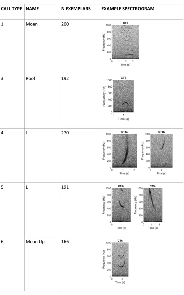
Mussoline, 2011). The quadratic discriminant function analysis (QDFA) is then used for the classification of all detected vocalization. For each vocalization, several attributes are calculated for the use in the QDFA (Baumgartner & Mussoline, 2011). Call attributes for classification include characteristics such as the start and end frequency, frequency range, duration, and the slope of frequency variation (Urazghildiiev et al., 2009). The classification analysis is done by comparing the detected sounds with a call library composed of seven different humpback whale call types (Table 1) and seven additional call types from other marine mammal species (Table 2) which vocalize in the same frequency range as humpback whales. The call library was compiled with a number of exemplars ranging between 153 and 332 for the humpback whale call types (Table 1) and between 139 and 321 exemplars for the other marine mammal call types (Table 2).

(11)

Table 1: Humpback whale call types, respective names, number of exemplars used in the library, and an exemplary spectrogram.

CALL TYPE NAME N EXEMPLARS EXAMPLE SPECTROGRAM

1 Moan 200

3 Roof 192

4 J 270

5 L 191

6 Moan Up 166

(12)

18 Low Frequency Down-Sweep

153

19 Low Frequency Moan

332

Table 2: Marine mammal species, call type, respective names, number of exemplars used in the library, and an exemplary of the spectrogram

SPECIES CALL TYPE NAME N EXEMPLARS EXAMPLE

SPECTROGRAM

Minke whale 30 Bioduck 213

Killer whale 31 Exited High Frequency Down Sweep

268

Weddell seal 32 Long downsweep 173

(13)

Crabeater seal 33 Pulsed moan 160

Leopard seal 34 Low trill 275

Leopard seal 35 High trill 139

Ross seal 36 Sirene call 321

The humpback whale call type 18 (Table 1), a low frequency downsweep, has acoustic characteristics that are similar to other baleen whale low-frequency downsweeps (Edds-Walton 1997, Baumgartner and Fratantoni 2008, and Ou et al., 2015). For this reason, in this study, this particular vocalization alone was not considered as representative of humpback whale acoustic presence (Appendix I, Figure 1). However, this vocalization can be representative of humpback whale acoustic presence when it occurs in combination with other humpback whale call types (Appendix I, Figure 2). Hence, in this study, only those downsweeps which were in combination with another known humpback whale vocalization were considered as a sign of humpback whale acoustic presence.

(14)

In a preceding study, a two-step evaluation analysis was applied to two different datasets. The first step evaluated a dataset composed of 30h of recordings and the second step evaluated a dataset composed of 150h of recordings. The aim was to tune the detection and classification parameters of LFDCS and the acoustic context filter. The thresholds resulted from this analysis were used in this study to automatically filter the data set. During the first evaluation step (30h dataset), the detection and classification parameters of LFDCS were tuned by comparing each of the humpback whale call detections with manually identified vocalizations in order to calculate the amount of false negative, true positive and false positive detections created by the software. Based on performance measures, i.e., recall ( Eq. 1, “the proportion of Real Positive cases that are correctly Predicted Positive”, i.e., the proportion of true positive cases which are correctly predicted) and precision (Eq. 2, “the proportion of Predicted Positive cases that are correctly Real Positives” i.e., the measure of accuracy of Predicted Positives), Powers (2011, p. 38), ten different parameter settings were chosen to be incorporated in the second step of the evaluation.

(1) Recall = tpr* = TP / RP** *True Positive Rate

** TRUE POSITIVE/REAL POSITIVE (2) Precision = tpa* =TP / PP** *True Positive Accuracy

** TRUE POSITIVE/PREDICTED POSITIVE

The aim of the second step (150h dataset) was to evaluate the detection efficiency on an hourly basis by comparing detection results with manually identified hourly humpback whale acoustic presence.

The parameter settings resulting in the best ratio between the probability of humpback whale acoustic presence and the probability of false negative hours were chosen.

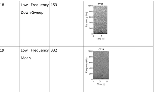
In order to further reduce the probability of false positive hours detected by LFDCS, an acoustic context filter was developed. False positive detections were expected due to the similarity of some humpback whale vocalizations with certain call types from other species (Table 3). Therefore, two conditions were used as a set for the acoustic context filter:

1. Within a recorded hour, the number of good quality detections (Mahalanobis Distance (MD;

i.e., the distance between a detected vocalization and the mean attribute vector of each call type present in the library) ≤ 2; Signal-to-Noise Ratio (SNR; i.e., the ratio between the amplitude of a vocalization and the amplitude of the background noise) ≥ 14 dB) of another species call type, which is similar to a humpback whale call type (Table 3), exceeds an hourly call rate threshold (i.e., four calls per hour).

(15)

2. In the same hour, the number of good quality humpback whale call detections (i.e., MD ≤ 2 and SNR ≥ 14) is lower than an hourly call rate threshold (i.e., six calls per hour).

If both conditions were fulfilled for the same recording hour, all the humpback whale detections which were similar to the other species’ call type were deleted from the relevant hour. Hence, false positive detected hours due to the presence of another species’ vocalizations could be reduced.

Additionally, for two parameters, MD and SNR, specific thresholds were chosen which in combination yielded the best ratio between the probability of humpback whale acoustic presence and the probability of false negative hours. For the MD a threshold of 2.5 was determined, and for the SNR a threshold of 13 dB was chosen.

The application of these thresholds resulted in the minimum probability of false negative hours, <20%, and simultaneous maximum probability of humpback whale acoustic presence, >70%, when the observed hourly call rate was at least ten detections per hour. Consequently, only the hours with a number equal or higher than ten detections of humpback whale vocalization were considered during the manual post-processing of the passive acoustic data in this study. The almost 18% of missed hours with humpback whale acoustically present were evaluated in terms of vocalization quality (i.e., SNR measurements). It was determined that more than 90% of the missed vocalizations had a SNR of below 10dB, which is equivalent to poor quality vocalizations commonly excluded from more detailed analyses (Magnúsdóttir et al., 2015; Rekdahl et al., 2015).

Table 3: List of humpback whale call types which are similar to certain other species’ call types.

HUMPBACK WHALE CALL TYPE

SIMILAR CALL TYPE FROM OTHER SPECIES

CT1 Leopard seal low trill (CT34)

Crabeater seal moan (CT33)

CT3 Ross seal sirene call (CT36)

CT5 Killer whale excited downsweep (CT31), Weddell Seal long downsweep (CT32)

CT6 Leopard seal low trill (CT34)

CT18 Minke whale Bioduck (CT30)

(16)

Manual post-processing analysis

The manual post-processing analysis was performed by a human analyst. A spectrogram was created using Raven Lite 2.0 to analyze the hours with automatically detected humpback whale vocalizations.

The spectrogram’s window size was set to 1025 samples, with 90% overlap and a discrete Fourier transform (DFT) size of 2048 samples. The scanning for humpback whale vocalizations has been done by visually and aurally inspecting 60 s windows with a frequency range between 0 and 1.8 kHz. Due to the restricted time available for this analysis only the even hours (hours 0, 2, 4, 6, 8, 10, 12, 14, 16, 18, 20, 22) of the recordings with presumed humpback whale acoustic presence were manually analyzed during the post-processing analysis. The spectrograms of every even hour with a presumed acoustic presence of ≥ 10 humpback whale detections were revised by the analyst to confirm the acoustic presence or report a false positive detection. The results of the post-processing analysis were reported on a Microsoft Excel sheet using the following numeric code: “1” for the confirmed acoustic presence of humpback whales and “0” for acoustic absence, i.e., a false positive hour.

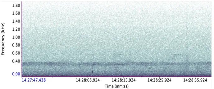
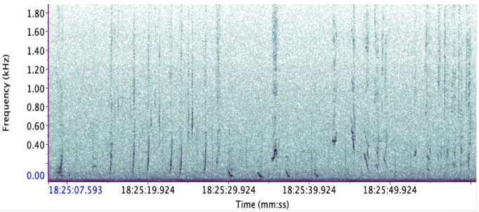
Humpback whale “social sounds” were defined as all the vocalization bouts without a defined pattern (i.e., see explanation of song category patterns; Figure 2). Vocalization bouts which showed a clear pattern have been considered as “song” (Figure 3, 4). In order to determine if a series of vocalizations were social sounds or a song, first was point out the presence of a repetitive pattern in the units, either identical or different units (Payne & McVay, 1971). Then the presence and length of inter-call intervals was investigated. The vocalization bouts were considered as social sounds when the repetitive pattern was not noticeable, and the inter-call interval was longer than 5 seconds. The vocalizations which showed a repetitive pattern of at least three phrases, with a call-interval shorter than 5 seconds were further analyzed to categorize the presence of songs (see Appendix III and Appendix IV for the detail of the categorization).

FIGURE 2: Spectrogram of humpback whale social sounds.

(17)

Humpback whale songs were further categorized into two distinct song categories: the preliminary song category and the complex song category. Complex song, from herein referred to as “song category 1” (Figure 3), was defined as those humpback whale vocalizations that were organized in a pattern of at least two different themes. On the other hand, humpback whale vocalizations which formed at least three repetitions of the same phrase type were considered as a preliminary song, from herein referred to as “song category 2” (Figure 4). Moreover, a quality evaluation of both social sounds and songs has been performed. The quality of vocalization was categorized into three levels: “1” for good quality, “2” for medium quality, “3” for poor quality.

FIGURE 3: Example of humpback whale song category 1. Two different themes are present, theme 2 in yellow and theme 1 in blue. The presence of two different themes define this as a song category 1, in purple.

FIGURE 4: Example of humpback whale song category 2. The same phrase, in red, is repeated for at least three times. This pattern composes a preliminary song, a song category 2.

Robustness of manual data post-processing

In order to evaluate the robustness of the manual post-processing by the analyst, a second analyst conducted the same manual post-processing analysis (blind) on a subset of the passive acoustic data.

The second analyst analyzed a period of 10 months, from 1 January to 28 October 2011, and applied the same rules for the classification of humpback whale vocalizations and the quality assessment.

The two analysts worked independently at all times. This aimed at avoiding possible interference between the two analysts. Both analysts used the same spectrogram settings in Raven to review the spectrogram and used the same numeric code for the classification. The robustness analysis was performed by cross comparing the results of both analysts.

THEME 2 THEME 1 THEME 1

THEME 1 THEME 1

SONG CATEGORY 2: same phrase repeated ≥ 3 times PHRASE A1

PHRASE A1 PHRASE A1

PHRASE A1

(18)

Humpback whale song analysis.

In order to analyze the acoustic presence of multiple humpback whale populations at the recording position between the years 2011 and 2012, a phrases catalogue was compiled first. This was accomplished by visually and aurally inspecting the recorded hours which were highlighted as including humpback whale songs. Due to the limitation imposed by the quality of the songs in the recordings, the song categorization analysis was focused on 12 hours of recordings from 12 different recording days for a total of 9 different songs.

Phrases catalogue

A phrase is defined as the repetition of multiple subphrases, which in turn consist of repetitions of one or more units (Payne & McVay, 1971). The composition of a phrase could be relatively subjective.

Cholewiak et al. (2013), provided the guidelines in order to help define which units belong to which phrase. The guidelines can be summed up as follows:

1. Consecutive units which show a similar shape should be kept together to form a sub-phrase.

2. Phrases should be defined by minimizing the occurrence of incomplete phrases either at the beginning or at the end of a sequence of similar phrases.

3. Transitional phrases are typically composed of subphrases from both the previous and the following themes, so they should be considered as such and not categorized as a new phrase.

4. Variation in the inner structure of the phrase should be taken into consideration as follows:

Variations in the phrase structure may involve the unit’s composition or the number of units that are repeated within the phrase. If the variation does not involve a drastic change such as entire unit compositions, it should be considered as a variation of the phrase previously categorized (see Appendix III).

For this study, the phrases were categorized as described above. Phrases that were composed of the same units and subphrases were considered as the same phrase and defined with an alphabetical code (e.g., A, B, etc.). If a variation in the number of units within the phrase was occurring, the phrase was considered as a part of the group of phrases which were showing a similar pattern (e.g., A1, A2, A3…see Appendix III). If the change affected the unit composition, and this new composition was found repeatedly, then the new phrase was enlisted in the catalogue. This procedure aimed to avoid cataloguing a transition phrase as a new phrase.

Theme catalogue

The repetition of similar phrases is defined as a theme (Payne & McVay, 1971). The same methodology of the phrase catalogue was applied for the theme categorization. Themes which were showing a

(19)

similar repetitive pattern in the phrase constitution were defined as a unique theme. A numeric code was assigned to them in order to define it as unique and distinguishable from the other themes (see Appendix IV).

When the change was involving the substitution of one phrase type, a new theme was established (e.g., Theme 1, 2…). If the modification in the composition involved a single call unit, a new theme sub- category was defined (e.g., 1A, 1B…see Figure 5, 6. Appendix IV). However, in order to better highlight the changes and the consistency in the theme sequences, the themes subcategories were gathered in broad categories (e.g., theme 1A, 1B, 1C, etc. all considered as Theme 1, see Appendix IV for the list of all the groups). If instead the change involved two or more call units, in one phrase as well as in multiple phrases, a new theme was defined.

FIGURE 5: Drawing of the theme type 1, in green. The theme is composed by the repetition of the phrase A1, in red.

FIGURE 6: Drawing of the theme type 1B, in orange. The theme is composed by the repetition of two phrases A1, in red, and a phrase A2, blue. This was considered as a sub-category of theme 1 because the change involved only a single unit.

Song catalogue

A song is defined as the repetition of distinct themes (Payne & McVay, 1971). In this study, a song was defined as the repetition of distinct themes with no pause in the singing behavior longer than 15 seconds. Each song was defined based on the theme and phrase composition. Each song was assigned

THEME 1

PHRASE A1 PHRASE A1 PHRASE A1

THEME 1B

PHRASE A1 PHRASE A2 PHRASE A1

(20)

a unique name. In order to avoid misunderstandings with the phrase and theme categories, to each song was assigned the name of a color (i.e., “Blue”, “Red”, etc..). Each song name reflects a specific theme and phrase compositions. If a change occurred in the theme (and so in the phrase) composition, a new song was defined and consequently a new name was assigned.

In a song session, the end of a song was defined by the presence of the first theme of the previous song. If the between two songs the pause in the singing behavior was longer than one minute the songs where considered as part of two different song session (Cholewiak et al., 2013).

Statistical analyses

With the purpose of testing for significant differences in the humpback whale acoustic presence between 2011 and 2012, first the distributions of the data were inspected. In order to test for the normal distribution of the humpback whale acoustic presence between January 2011 and September 2012, the Shapiro-Wilk normality test, the “shapiro.test’ function in the R package “ggpubr” (The R Project for Statistical Computing) was used.

Since the humpback whale acoustic presence was not normally distributed, the nonparametric Kruskal- Wallis test, “Kruskal.test” function in R package “stats” (The R Project for Statistical Computing), was used to compare the humpback whale relative acoustic presence within years. As a post-hoc analysis the Pairwise-Wilcox-Test, “pairwise.wilcox.test” function in R, R package “multcomp” (The R Project for Statistical Computing) was used to compare the humpback whale acoustic presence among months (Appendix II, Figure 1 & 2).

Mean and the standard deviation of the monthly and yearly humpback whale acoustic presence was calculated using the “SummarySE Function” included in the R package “Rmisc” (The R Project for Statistical Computing).

Results

Robustness of the manual post processing analysis

The high level of agreement between the two analysts shows the robustness of the manual post- processing analysis. A total of 1024 hours with assumed humpback whale acoustic presence were reviewed.

The level of accordance between the two analysts was calculated by dividing the number of equally classified hours by the number of in total revised hours. The number of distinctly classified hours were divided by the number of the total revised hours, and the level of disagreement was calculated.

(21)

Of the 1024 hours analyzed by both analysts, the percentage of agreement between the two was 96.4%, representing 987 hours of recordings in total (Figure 7a). Of the 987 hours in which the analysts agreed, 575 hours, 56.2%, represent the agreement in humpback whale acoustic absence (i.e., the percentage of false positive hours detected by the LFDCS) and 412, 40.2%, represent the agreement in humpback whale acoustic presence, i.e., the percentage of true positive hours detected by the LFDCS (Figure 7a). Additionally, the percentage of disagreement was calculated at 3.6%, for a total of 37 hours of recordings. Of these 37 hours in which the analysts disagreed, 41% of the disagreement (15 hours) was in the acoustic absence, and 59% (22 hours) was related to the acoustic presence (Figure 7b).

FIGURE 7: Detail of the agreement level during the manual post-processing analysis. a) the overall level of agreement and disagreement. Given a disagreement of 3.6% between the analysts (b) represent the specific percentages of the reasons in the disagreement between the analysts.

Humpback whale acoustic presence.

2011

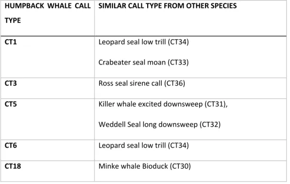
Overall, in 2011, 446 hours with acoustic presence of humpback whales were confirmed. Humpback whale vocalizations were found from January to December. The peak of acoustic presence was between 1 April and 27 May 2011 (Figure 8). From 13 January to 25 March, humpback whale vocalizations were detected irregularly (Figure 8). From 26 March to 25 May humpback whales were acoustically present almost continuously, resulting in 61 days with at least one hour of humpback

a b

(22)

whale acoustic presence. The monthly average of hours with humpback whale acoustic presence was calculated in 169.1 hours/month. Only on 26 April the humpback whales were acoustically absent. In the period between 28 May and 31 December humpback whales were sparsely acoustically present during few hours per month. In this period, the average hours per month with humpback whale acoustic presence was calculated in 3.9 hours/month (Figure 8).

FIGURE 8: Heatmap of the humpback whale acoustic presence for the year 2011. The yellow to red color scale describe the amount of number of recorded hours with humpback whale acoustic presence. In white are the days with humpback whale acoustic absence. In grey are the days not present in the dataset.

2012

In 2012, 240 hours of acoustic presence for humpback whales were confirmed. Humpback whale vocalizations were present from February to June, and again in August. The first evidence of humpback whale acoustic presence was recorded on 22 February. The peak in the number of hours with acoustic presence per day was between 1 March and 13 April (40 days with humpback whale acoustic presence) with only three days, between 29 March and 2 April, with no humpback whale vocalizations (Figure 9).

In this period, the average hours per month was calculated in 176.1 hours/month. From 13 April to 7 May 2012, there were no data available due to a hydrophone technical failure. From 7 May to 17 September 2012, only for two days, 7 May and 2 June 2012, humpback whale acoustic presence was confirmed (Figure 9).

1 3 6 9 12

(23)

FIGURE 9: Heatmap of the humpback whale acoustic presence for the year 2012. The yellow to red color scale describe the amount of number of recorded hours with humpback whale acoustic presence. In white are the days with humpback whale acoustic absence. In grey are the days not present in the dataset.

For both years 2011 and 2012, the data were not normally distributed (p-value <2.2e-16) and the monthly humpback whale acoustic presence resulted to be significantly different (Table 4).

Table 4: Results of the Kruskal-Wallis Test for the acoustic presence among different months.

Kruskal-Wallis Test p-value Year 2011 - Acoustic Presence < 2.2e-16 Year 2012 - Acoustic Presence < 2.2e-16

The P-values reported for both years 2011 and 2012 showed a significant difference within the humpback whale acoustic presence throughout the months analyzed. For the year 2011, the humpback whale acoustic presence was not significantly different in April and May (p-value= 0.0735) but there was a significant difference between these two months and the rest of the months (Appendix II, Figure 1).

In the following year the humpback whale acoustic presence was not significantly different between March and April (p-value = 0.055) but was instead significant between these months and the other months analyzed in 2012 (Appendix II, Figure 2).

For the year 2011, the mean for the humpback whale hourly acoustic presence was calculated to be 0.295 ± 0.456 hours with acoustic presence/recorded hours. The months with the highest percentage

1 3 6 9 12

(24)

of humpback whale acoustic presence were April and May 2011, for which the hourly relative acoustic presence was calculated in 0.902 and 0.954 hours with humpback whale acoustic presence/recorded hours respectively (Figure 10). For the following year (2012) the mean was 0.303 ± 0.460 hours with humpback whale acoustic presence/recorded hours, and the months with the highest hourly relative acoustic presence were March with 0.768 and April with 0.919 hours with humpback whale acoustic presence/recorded hours (Figure 10, Appendix II Table 1)

FIGURE 10: Humpback whale relative acoustic presence (hours with humpback whale acoustic

presence/recorded hours) andstandard deviation for the years 2011 and 2012. Only the upper section of the standard deviation was plotted because the acoustic presence cannot have negative values.

Categorization of humpback whale songs

2011

The first humpback whale song detected was on 5 April and the last one on 24 May (Figure 11a). After 24 May no song was recorded, and humpback whale vocalizations were rarely present. A total of 77 hours with humpback whale songs were documented. Within those hours, 56 were described as “song category 1” and 22 as “song category 2” (Figure 11a and 11b respectively). More specifically, in April, 25 recorded hours with songs category 1 and 5 recorded hours including songs category 2 were found.

In May, 31 recorded hours with songs category 1 and 17 hours with songs category 2 were described (Figure 11a, b). The interval of days including the highest number of hours with humpback whale songs was between 28 April and 1 May, and between 14 May and 19 May 2011 (Figure 11a, b). Within these two periods the average of recorded hours including humpback whale songs was 3 hours per day (Figure 11a, b). The concentration of humpback whale songs decreased between 19 May and 24 May 2011. On 24 May, the last song was detected marking the end of the humpback whale song period recorded in the sampling area for the rest of 2011 (Figure 11b).

(25)

FIGURE 11: Heatmap of the numbers of recorded hours with humpback whale songs (category 1 & 2) for the year 2011. a) red and orange scale color, heatmap describing the number of hours with humpback whale song category 1. b) purple and pink scale color, heatmap describing the number of hours with humpback whale song category 2.

During April in 2011, the average of hours with humpback whale songs category “1” was calculated in 0.113 hours with humpback whale song/recorded hours, from herein referred to as “song/hour”, and the standard deviation in ± 0.318. In the same month, the average of hours with songs category “2”

was calculated in 0.025 ± 0.156 song/hour (Figure 12a). During May 2011, the average of hours with song category “1” was 0.192 ± 0.395 song/hour and for the hours with songs category “2” was 0.116 ± 0.342 song/hour (Figure 12b).

FIGURE 12: Relative number of recorded hours with humpback whale song category 1 (dark blue) and song category 2 (light blue) detected in 2011. Only the upper section of the standard deviation was plotted because the song category abundance cannot have negative values.

a

b

a) b)

(26)

2012

Overall, for the year 2012, 56 hours including humpback whale songs were verified. Of these, 39 were described as song category “1” and 17 as song category “2” (Figure 13a and 13b respectively). In March, 16 hours including song category “1” and 11 song category “2” were confirmed. In April, 23 hours containing song category “1” and six song category “2” were detected (Figure 13a and 13b respectively). The first humpback whale song was detected on 12 March 2012 (Figure 13a, b). The days with the highest number of recorded hours with humpback whale songs occurred on March 12 and 14, with the peak occurred on 8 May 2012 (Figure 13a, b). Between 18 and 25 March, as well as from 27 March to 2 April, no humpback whale songs were recorded (Figure 13a, b).

FIGURE 13: Heatmaps of the numbers of recorded hours with humpback whale songs (category 1 & 2) for the year 2012. a) red and orange scale color, heatmap describing the number of hours with humpback whale song category 1. b) purple and pink scale color, heatmap describing the number of hours with humpback whale song category 2. In grey the days during which the hydrophone did not record.

In March 2012, the average hours with humpback whale songs category “1” was 0.083 ± 0.277 song/hour and for the song category “2” was 0.058 ± 0.235 song/hour (Figure 14a). In April 2012, the average of song category “1” was 0.238 ± 0.453 song/hour and for the song category “2” was 0.093 ± 0.293 song/hour (Figure 14b).

a a b

(27)

FIGURE 14: Relative number of hours with song category 1 (dark blue) and song category 2 (light blue) detected in 2012. Only the upper section of the standard deviation was plotted because the song category cannot have negative values.

Humpback whale song analysis.

Phrases

.

Altogether, during the two years that were analyzed for this study 469 phrases were categorized. The phrases were grouped in 12 different phrase categories (following an alphabetical order from A to L) and 14 sub-categories (Figure 15, see Appendix III).

Overall, the most common phrases were A1, A2, B1 and G2 (Figure 15). The phrase type A1 and A2 were the most present with 85 and 80 times respectively, then the phrase G2 with 52 times and the B1 type with 50 times (Figure 15). In 2011 the number of phrase category and subcategories present was higher than in 2012, 16 and 11 respectively. Moreover, two phrases (G2 and H1) were recorded more than 25 times, and the phrase G2 was present for 52 times; nonetheless, in 2012, the number of phrase type used above 25 times were four (A1, A2, B1 and B2), and three of these (A1, A2, B1) were recorded for at least 50 times (Figure 15).

a) b)

(28)

FIGURE 15: Detail of all the number of phrases and subphrases categorized in the year 2011 and 2012. On the x-axis are the phrase types present in the two years, on the y-axis the number of phrases calculated during the two years.

The phrases repertoire variated substantially from 2011 to 2012. In both years only 0.04% (1 of 26 phrases) of the total number of phrases were present. The only phrase present in 2011 and 2012 was the phrase type A2 (Figure 16, highlighted in red). The repertoire of humpback whales in the eastern Weddell Sea changed almost completely. Hence, a high level of unicity among the phrase repertoire was reported. Additionally, the usage of the phrase A2 changed enormously. During 2011 the phrase was present three times in 2012 for 80 times (Figure 16). Furthermore, in 2012 also other A type subcategories (A1 and A3) were present. Phrase type A1, A2 and A3 represented the most commonly sung phrases in both years (Figure 16).

FIGURE 16: Detail of all the number of phrases and subphrases categorized in the year 2011 and 2012.

Highlighted in the red box is the only phrase type (A2) which is shared between the two years. On the x-

A2 C1 C2 D1 D2 D3 E F G1 G2 H1 H2 H3 L1 L2L2 J

PHRASE TYPE A1 A2 A3 B1 B2 B3 K1 K2 K3 K4 L

PHRASE TYPE

PHRASE TYPE I 1 I 2

A2 C1 C2 D1 D2 D3 E F G1 G2 H1 H2 H3 L1 L2L2 J

PHRASE TYPE PHRASE TYPE I 1 I 2

I 1 I 2 A2 C1 C2 D1 D2 D3 E F G1 G2 H1 H2 H3 L1 L2L2 J

PHRASE TYPE

PHRASE TYPE I 1 I 2

(29)

axis are the phrase types present in the two years, on the y-axis the number of phrases calculated during the two years.

The analysis of the daily usage of each phrase underlined the differences between the two years.

Therefore, two different trends are appreciable (Figure 17).

2011

In 2011, five days 13, 17, 25, 28 April and 19 May were analyzed in detail. Four of the five days showed almost the same phrase type usage (Figure 17). During all the five days only the phrases G1 and G2 were present. Within four days (13, 25, 28 April and 19 May) the phrase type G1, G2, H1, H2, H3 were present consistently. On 25 and 28 April the only phrase (A2) present in both 2011 and 2012 was reported (Figure 16, 17). Remarkably, on 17 April 2011 the phrase repertoire drastically changed. In addition to the phrase types G1 and G2, the phrases category C, D and F were present (Figure 17). The fluctuation in the repertoire present in these days might be indicative of the acoustic presence of two different humpback whale populations in the eastern Weddell Sea.

2012

During this year an increasing trend in the number of different phrases present was appreciable. The days 12, 14, 13 March and 4, 5, 9 and 12 April analyzed in detail. In the 7 days analyzed the phrases A1 and A2 were present consistently. As the austral summer ended the number of phrases which were present during this period gradually increased. On 12 March only four different phrases were present while on 12 April the number of distinct phrases present were 10 (Figure 17). Furthermore, the number of phrases repeated each day increased as well as the variability of the repertoire (Figure 17). Between 12 March and 12 April, the repetition of phrases A1 and A2 rose from 3 and 9 times per day to 27 and 23 respectively (Figure 17). For the phrase types B1 and B2 the same trend was appreciable (Figure 17).

(30)

FIGURE 17: Heatmap of all the number of phrases and subphrases categorized in the year 2011 (left) and 2012 (right). On the x-axis are reported the days on which the phrases were present. On the y-axis are listed all the phrases subcategories present during the days analyzed.

Themes

.

Altogether, during the two years analyzed 162 themes were present. The themes were categorized into 11 different categories (following a numerical order from 1 to 11, see Appendix IV for theme composition). The number of theme categories (11) were less than the phrase categories (12) due to the phrase type “E” which was present two time but on distinct moments during 17 April, therefore did not form a theme.

Globally the themes 1, 2, 4 and 5 were the most frequent. Above all, the most common themes were theme types 1 and 2, present for 57 and 34 times respectively (Figure 18, 19). In 2011 the number of distinct themes was higher than in 2012, 7 and 5 respectively. However, the total amount of themes was higher in 2012, 110, than in 2011, 52 (Figure 18).

04/13/2011 04/17/2011 04/25/2011 04/28/2011 05/19/2011 03/12/2012 03/14/2012 03/15/2012 04/04/2012 04/05/2012 04/09/2012 04/12/2012 Month/Day/Year

HH H

G I IJ K KK KL

G EF DD DC CB BB AA A1

1 1 1 1 1 1 12 2

2 2

2

23 3 3 3 34

(31)

FIGURE 18: Number of the different theme types categorized in 2011 and 2012. On the x-axis are the theme types present in the two years, on the y-axis the number of themes calculated during the two years.

FIGURE 19: Spectrograms of the most common theme types categorized in both years: a) theme 1 and b) theme 2

Likewise, as reported in the phrase analysis, between 2011 and 2012 the repertoire of themes changed drastically. In both years only theme 1 was consistently present, rising from one (in 2011) to 56 repetitions, in 2012 (Figure 20).

a

b

(32)

FIGURE 20: Number of the different theme types categorized in 2011 and 2012. Highlighted in the red box is the only theme type (Theme 1) which is shared between the two years. On the x-axis are the theme types present in the two years, on the y-axis the number of themes calculated during the two years.

2011

On the five days analyzed in 2011, only the theme type 4 was present consistently. Themes 4 and 5 were present on four (13, 25, 28 April and 19 May) of the five days analyzed. On 17 April the theme repertoire changed drastically. Theme 8 and theme 9 were indeed present only on 17 April (Figure 22).

On 28 April the only common theme between 2011 and 2012, theme 1, was present.

2012

In 2012 the high consistency of the theme type presence was appreciable. Theme 1 and 2 were present consistently. Each theme (1 and 2) was reported to be sung seven times on the first day analyzed (Figure 21). Then the theme repetitions decreased to one (theme 2) and three (theme 1) on 14 and 15 March. On 12 April increased again to 16 times for theme 1 and seven times for theme 2 (Figure 21).

For theme 3 the same trend of theme 1 and 2 was observed. On 15 March the theme 3 was present for one time, then on 12 April was present for 16 times (Figure 21).

(33)

FIGURE 21: Heatmap of all the number of themes categorized in the year 2011 (left) and 2012 (right). On the x-axis are reported the days on which the themes were present. On the y-axis are listed all the themes categories present during the days analyzed.

Songs

.

The song composition analysis showed a net difference between 2011 and 2012. Between the two years the song repertoire was entirely revolutionized, no themes or phrases among the different songs were shared. Over the 2312 hours of recording evaluated in this study, 135 hours including songs were identified. Of these, 12 hours including good quality songs were analyzed in detail. In total, 9 different songs were identified and further categorized, three in 2011 and six in 2012. Overall the same trends described above in the phrases and themes analysis was encountered also in the song analysis. In 2011 the Blue song was present for four days while the Red song on two days; the Yellow song was present only on one day, during which no other songs were present. In 2012, the complexity and length in the song structure increased as the Austral summer ended.

2011

For the year 2011, three different songs were identified and categorized. The songs identified in this year were the Blue, the Red and the Yellow. The Blue song was present on 13, 25, 28 April and 19 May while the Red song was sung on 13 and 28 April. On 17 April only the Yellow song was present.

The Blue song was composed by two themes, typically in the order theme 4 and theme 5 (Figure 22a).

The sequence of phrases which composed the song was: “G-G-H-H” (Figure 22a). On 13 April and 19 May, two distinct sets of multiple Blue songs were present; hence two song sessions were defined.

I 1 I 2

04/13/2011 04/17/2011 04/25/2011 04/28/2011 05/19/2011 03/12/2012 03/14/2012 03/15/2012 04/04/2012 04/05/2012 04/09/2012 04/09/2012

Month/Day/Year

04/12/2012

(34)

Specifically, on 13 April the song session was composed by the repetition of three Blue songs and on 19 May by four Blue songs.

The Red song was instead composed of theme 5 first and then theme 4 (Figure 22b). The song was present in two different “forms”: 1) On 13 April a “long version” composed by the repetition of phrase H for six times and then the phrase G repeated for two times was recorded. 2) On 28 April a “short version” composed by the sequence H, H, G, G was present (Figure 22b).

In contrast, the Yellow song was composed of four distinct themes: 4, 8, 6 and 9, and it was the longest song recorded in the year. The song was built by the phrases G, G, C, C, C, F, F, D, D, D, and represented the only song of the year which had a composition drastically diverse from all the other songs (Figure 22a, b, c).

FIGURE 22: Spectrogram and drawing of the Blue (a), Red (b) and Yellow (c) songs. On the top part of the image are the songs representing the humpback whale population “A”, on the bottom part of the image the song representing the humpback whale population “B”.

2012

In 2012 a higher number of songs (6) was recorded. The songs recorded for the first time in March (i.e., Orange and Magenta) showed an increasing trend in length and complexity with the approaching of the Austral winter. In April, the new songs were all composed of the repetition of three distinctive themes. Themes 1, 2 and 3 were the main themes sung this year.

The Magenta and Orange songs represented the baseline from which the building process started. The building process firstly showed an increasing trend in the number of phrases repeated each time the

THEME 4

PHRASE G repeated PHRASE H Repeated

PHRASE H repeated PHRASE G repeated

b

BLUE SONG

YELLOW SONG

RED SONG Population A

Population B

THEME 4 PHRASE G repeated

THEME 8 PHRASE C repeated

THEME 6 PHRASE F repeated

THEME 9 PHRASE D repeated THEME 4

PHRASE G repeated

a b

c

5

(35)

song was sung. Secondly, the complexity of the “native” songs increased due to the insertion of new distinctive themes.

MAGENTA TO SILVER SONG

On three different days, 14 March, 4 and 5 April, the Magenta song was recorded. The Magenta song was composed by the themes 2 and 1. A short version of the song was sung on 14 March and 4 April, and it was composed by the sequence of phrases B, B, B, A, A, A, A, (Figure 23a). On 5 April, an extended version of the Magenta song was recorded. The phrase sequence was built using six phrases B and seven phrases A (Figure 23b).

On 12 April the Silver song was recorded, and it might represent the maturation of the Magenta song.

The Silver song and the Magenta song shared the same theme order, but the Silver song presented the insertion of the phrase N repeated multiple times between the phrases B and A. The phrase sequence was B – N – A, with each phrase type repeated several times (Figure 23c).

FIGURE 23: Spectrogram and drawing of the Magenta song, short (a) and extended version (b), and Silver song (c)

PHRASE B repeated PHRASE N repeated PHRASE A repeated

PHRASE A repeated PHRASE B repeated PHRASE L repeated

THEME 2

THEME 1

PHRASE B repeated PHRASE A repeated

a

THEME 2 PHRASE B repeated

THEME 1 PHRASE A repeated

b

a

b

c

MAGENTA SONG (short version)

MAGENTA SONG (extended version)

SILVER SONG

(36)

ORANGE TO GREEN, BROWN AND PINK SONGS

On 12 March the Orange song was recorded for the first time. The song was composed of two distinct phrases, A and B. On 12 and 15 March and 4 April the phrase sequence was A, A, B, B, B (Figure 24a).

However, on the 4 April the song was also recorded in a longer version, composed by the phrases A, A, B, B, B, B. On 9 April the longest version of the Orange song was recorded, and it was composed by the sequence A, A, A, A, A, A, A, A, B, B, B, B (Figure 24b).

On 4 April the first variation of the Orange song was present. The Green song started with the repetition of the phrases A and B and ended with the phrase type L repeated for three times (Figure 24c, phrase L in the purple boxes). The Orange song was composed by the repetition of the phrases A and B only. Consequentially the Green song may represent a possible derived form of the Orange song (Figure 24a, b, c).

On 12 April two new distinctive forms of the Orange song were recorded. The Brown and the Pink song developed the insertion of the same phrase N but in different position in the song structure. In the Brown song the phrase N was present at the beginning (Figure 24d) while in the Pink song at the end (Figure 24e). This phrase composition was already found in the Silver song, but in a completely different order of the phrase and theme; therefore, the Silver song was considered as a variation of the Magenta song, and the Brown and Pink songs as a variation of the Orange song.

FIGURE 24: Spectrogram and drawing of the Orange song, short (a) and extended version (b), then the Green (c), the Brown (d) and the Pink (e) songs.

THEME 1 THEME 2

PHRASE A repeated PHRASE B repeated

THEME 1

PHRASE A repeated PHRASE B repeated

THEME 2

PHRASE A repeated PHRASE B repeated PHRASE B repeated PHRASE A repeatedPHRASE L repeatedPHRASE L repeated

PHRASE A repeated PHRASE B repeated PHRASE N repeated

PHRASE B repeated

PHRASE N repeated PHRASE A repeated

BROWN SONG GREEN SONG

PHRASE A repeated PHRASE B repeated PHRASE N repeated

PINK SONG ORANGE SONG (short version)

ORANGE SONG (extended version) a

b

c

d

e

Sari Mangia Woods

Preliminary assessment of the acoustic presence of multiple humpback whale (Megaptera novaeangliae) populations in

the eastern Weddell Sea in 2011 and 2012.

Sari Mangia Woods

Table of Contents

Abstract

Aims & Research questions

Overall aim:

Research question:

Introduction

Materials and methods

Data collection.

Data analysis.

b

b

Automated data processing

Manual post-processing analysis

Robustness of manual data post-processing

Humpback whale song analysis.

Phrases catalogue

Theme catalogue

Song catalogue

Statistical analyses

Results

Robustness of the manual post processing analysis

Humpback whale acoustic presence.

Categorization of humpback whale songs

Humpback whale song analysis.

Phrases

Themes

a

b

Songs