Contents
0.1 Preliminary Schedule . . . 4
0.2 Literature . . . 4
0.3 Course Content . . . 5
1 What is Solid-State Physics about? 6 2 Lattices 8 2.1 Why we care about symmetries . . . 8
2.2 Crystal lattices . . . 9
2.2.1 Crystal lattices in 2D . . . 9
2.2.2 Crystal lattices in 3D . . . 10
2.2.3 Unit cells . . . 12
2.3 Reciprocal Lattice . . . 12
2.3.1 Fourier transforms and Periodic Boundary Conditions (PBC). . . 14
3 Separation of Lattice and Electrons and Lattice Dynamics 18 3.1 Adiabatic Approximation: Separate Hamiltonians for Electrons and Ions . . 18
3.1.1 Equilibrium Positions of the Ions: How the Lattice arises . . . 19
3.1.2 Add back the kinetic energy of the ions . . . 20
3.2 Lattice Dynamics and Phonons . . . 23
3.2.1 Phonons in Solids . . . 24
3.2.2 Creation and Annihilation operators for phonons . . . 27
3.2.2.1 Linear phonon dispersion for some special modes . . . 29
3.2.3 Thermodynamics of Phonons . . . 31
3.2.4 Lattice Stability and Melting . . . 34
3.2.5 Anharmonic Effects . . . 35
4 Electrons in a Periodic Potential 37 4.1 Bloch’s theorem . . . 37
4.2 Nearly Free Electrons . . . 39
4.2.1 Schr¨odinger equation for Bloch waves in Momentum space . . . 39
4.2.2 Free electrons and the Periodic Lattice . . . 40
4.2.3 Weak potential: Perturbation Theory . . . 41
4.3 Tight-Binding Bands . . . 43
4.3.1 Wannier functions . . . 45
4.4 Thermodynamics of Non-interacting Electrons . . . 46
4.4.1 Density of States and Sommerfeld approach . . . 48
4.4.2 The Free Electron Gas . . . 50
4.4.3 Metals – Insulators – Semiconductors . . . 52
4.5 Electrons in an electric field – and a periodic potential . . . 52
4.5.1 Weak field, simplest approximation . . . 52
4.5.1.1 Effective mass and⃗k⋅ ⃗p perturbation theory. . . 53
4.5.2 Replacing spatial dependence by time dependence: anomalous velocity 54 5 Green’s functions for Many-Body Systems 57 5.1 Some aspects of Second Quantization. . . 57
5.2 Linear Response Theory . . . 57
5.3 Schr¨odinger Time-evolution Operator and One-particle Green’s function . . 60
5.3.1 Green’s “functions” as operators . . . 62
5.4 Tools, Rules, and Technical Details concerning Green’s functions . . . 62
5.4.1 Advanced and Causal Green’s functions . . . 62
5.4.2 Equation of Motion, Frequency Domain . . . 63
5.4.2.1 Example: Green’s function for non-interacting particles. . . 64
5.4.2.2 Slight shift ofω off the real axis to ensure convergence . . . 64
5.4.3 Lehmann representation and Spectral Density . . . 65
5.4.3.1 Example: Spectral density for non-interacting particles . . . 66
5.4.4 Some exact Relations, Kramers-Kronig . . . 67
5.4.5 “The” Green’s function: Causal one particle Green’s function. . . 68
5.5 From particle to quasi particle, self energy, Fermi liquid . . . 69
5.5.1 Dyson equation and self-energy for one-particle problems . . . 69
5.5.2 Self-energy for interacting systems, Fermi-liquid theory . . . 71
5.6 Perturbation Theory: Adiabatic switching on of the interaction . . . 73
5.6.1 Gell-Mann and Low theorem . . . 73
5.6.2 Expectation values of the interacting system . . . 74
5.6.3 Wick’s Theorem . . . 76
5.6.4 Feynman diagrams . . . 77
5.6.5 Dyson equation and Self energy: Summing some kinds of diagrams to infinite order:. . . 79
5.6.6 (Self-Consistent) Hartree Approximation to the Hubbard model . . . 81
5.6.6.1 Via equations of motion. . . 81
5.6.6.2 Via diagrams . . . 82
5.6.6.3 Self Consistency . . . 84
5.6.7 Note on finite Temperatures . . . 85
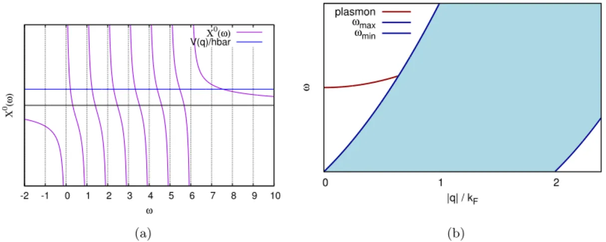
5.7 Response functions. . . 85
5.7.1 Charge-charge correlation . . . 85
5.7.1.1 Equation of motion for the charge susceptibility – non- interacting case. . . 86
5.7.1.2 Equation of motion for the charge susceptibility – with in- teraction . . . 87
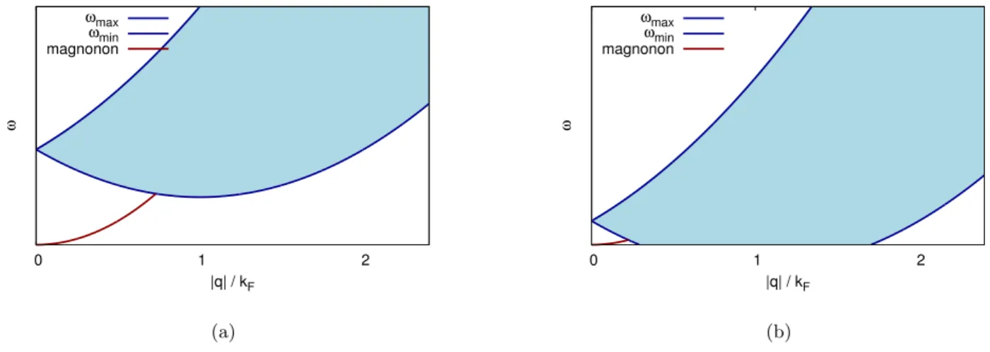
5.7.2 Magnetic susceptibility . . . 90
5.7.2.1 Magnetic susceptibility with interaction . . . 91
5.7.3 Nesting as an indicator for potential order . . . 92
6 Symmetry breaking: Magnetism and Superconductivity 94
6.1 Magnetism. . . 94
6.1.1 Paramagnetism: Existing moments without interactions . . . 94
6.1.1.1 Magnetic susceptibility of non-interacting electrons . . . 94
6.1.1.2 Magnetic susceptibility of non-interacting spins . . . 95
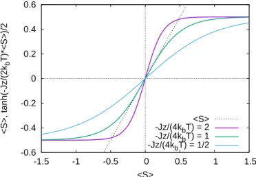
6.1.2 Interacting moments and ordered states . . . 96
6.1.2.1 Mean-field treatment . . . 97
6.1.2.2 Excitations and Validity of the Mean-field Treatment . . . . 99
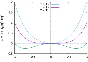
6.2 (Ginzburg-)Landau Theory . . . 100
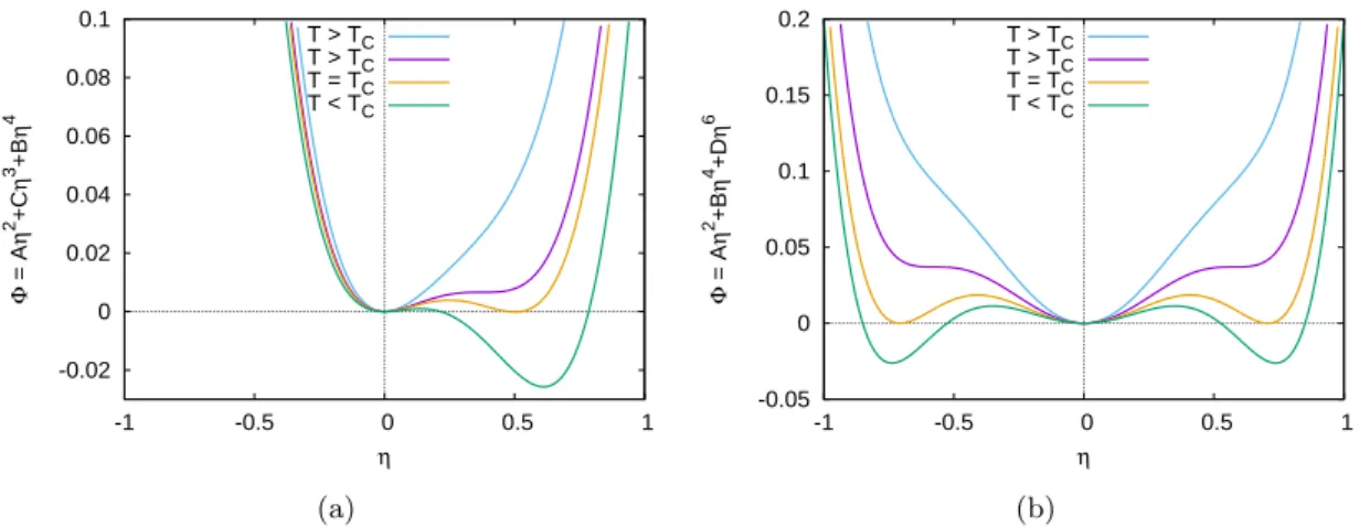
6.2.1 Second-order transition. . . 102
6.2.2 Weakly first-order transitions . . . 103
6.2.3 Inhomogeneous States and gradients in the order parameter . . . 104
6.3 Superconductivity . . . 104
6.3.1 Phonon-mediated Electron-Electron Interaction . . . 105
6.3.2 BCS Theory of Superconductivity . . . 107
6.3.2.1 BCS Gap equation . . . 110
6.3.2.2 ‘Unconventional superconductivity’ with momentum- dependent gap . . . 111
6.3.3 Ginzburg-Landau Theory of Superconductivity . . . 112
0.1 Preliminary Schedule
April 4 Introduction: Content, organisation (Exercises!), start symmetries: Bravais lattices in 2D, Crystal structures
April 8 Fourier transform, reciprocal lattice, Brillouin zones April 11 Adiabatic approximation, start chemical bonds April 15 chemical bonds, start phonons
April 18 phonons
April 22 Phonon dispersion, thermodynamics of phonons, density of states April 25 metling, anharmonicity, Bloch theorem
April 29 nearly free electrons
May 2 tight-binding, Bloch/Wannier states
May 6 Many-body states for electrons, density of states May 9 specific heat of electrons, velocity in an electric field
May 13 Second quant., Green’s functions: Dirac picture, Linear response, one-particle GF May 23 ret. and adv. Green’s function in frequency space, independent particles
May 27 Causal one-particle GF; spectral density, Kramers-Kronig, Lehmann May 30 GF for one-particle problem with impurity, interacting self energy
June 3 Fermi-liquid theory
June 6 Perturbation theory until contractions
June 10 Wick’s theorem and Feynmann diagrams, up to rules
June 13 Dyson equation, self-consistent mean field, Hartree for Hubbard model June 17 Mirco
June 20 cancelled
June 24 other Green’s functions, charge susceptibility June 27 magnetic susceptibility
July 1st finish magnetic susceptibility, magnetism July 4 Magnetism: Mean-field for Heisenberg/Ising July 8 Landau theory of symmetry breaking
July 11 phonon-mediated electron-electron interaction, BCS Theory July 15 Superconductivity
0.2 Literature
• For Physics: N.W. Ashcroft and N.D. Mermin: Solid State Physics, Sauders College Publishing, 1976.
• For Theoretical Physics: Daniel I. Khomskii , Basic Aspects of the Quantum Theory of Solids: Order and Elementary Excitations, Cambridge University Press, 2010
• For Theoretical Physics: Roser Valent´ı, lecture notes (mostly in German), http://itp.uni-frankfurt.de/ valenti/WS14 15.php
• For Math, Formalism and the more advanced physics: A. Muramatsu, Solid State Theory,
http://www.itp3.uni-stuttgart.de/lehre/Archiv/ss13/solidstatetheory/solidstatetheory.en.html
• For Math and Formalism (and some of the more advanced physics): C. Timm, Viel- teilchentheorie (in German),
http://www.physik.tu-dresden.de/ timm/personal/teaching/vtt w10/
• Linear-response Theory and equation of motion for Green’s functions: W. Nolting, Fundamentals of Many-body Physics, Springer, 2009
• for Feynman diagrams: Richard D. Mattuck, A Guide to Feynman Diagrams in the Many-Body Problem, Dover Books on Physics
• Field-Theory focussed, mostly more advanced:, A. Altland and Ben Simons, Condensed Matter Field Theory, Cambridge University Press, 2006
0.3 Course Content
• Periodic Lattices
– Lattice symmetries: translational and other – Oscillations around equilibrium: Phonons
• Electrons in periodic potentials
– Very short review second quantization – Bloch’s theorem
– Nearly free electrons to tight binding
– Many-body states for fermions and bosons: Some statistical physics
• Electron-electron interactions
• Electron-phonon interaction
• Models
– How they are developed – Where they are valid – What we learn from them
• Properties of Solids – Magnetism
– Superconductivity – Excitations
1 What is Solid-State Physics about?
Condensed-Matter Physics: deals with temperatures and energies ”on human scales”.
• Soft Condensed Matter: e.g. liquids, Molecules, biophysics,. . ..
• Solid-state Physics(”hard” condensed matter): crystals
– glasses: locally ordered, globally disordered, usually metastable states
– quasicrystals: local rules, symmetries (e.g. five-fold rotation) that do not work out globally
– ”normal” periodic lattices
Types of particles and interactions are in principle known: particles treated are electrons and the nuclei of the atoms, often even ionic cores that include tightly bound electrons. The relevant interaction is the electromagnetic one, in particular Coulomb interaction between charged ions and electrons. The weak and strong forces are not treated, because they act only on the ”inside” of the nucleus, and gravity is neglected as well.
Typical Hamiltonian is then given by the kinetic energies of electrons and nuclei in addi- tion to the interaction:
H= ∑
¯i electrons
ˆ⃗ p2 2m + ∑
¯i nuclei
ˆ⃗ P2 2Mi +e2
2 ∑
¯i,j electrons
1
∣rˆ⃗i−ˆ⃗rj∣+e2
2 ∑
¯i,j nuclei
ZiZj
∣Rˆ⃗i−Rˆ⃗j∣−e2 ∑
¯i,j electron-nucleus
Zj
∣rˆ⃗i−Rˆ⃗j∣ (1.1) Capital letters denote operators for nuclei and lower-case ones those for electrons. Relativis- tic electrons obey the Dirac equation, but energy scales in condensed matter are far below the rest mass of the electron (the lightest particle in question), a non-relativistic treatment is thus usually sufficient. Relativistic effects can be relevant in some cases, but it is then sufficient to treat them on the level of the Pauli equation. This is still in the non-relativistic limit of the Dirac equation, but relativistic effects are included in perturbation theory in terms of mc12. Such an approach yields spin-orbit coupling.
The only parameters entering this Hamiltonian are the chargesZiand the massesMi, with the latter being largely proportional to the former. (The differences between isotopes can be relevant for phonons, though.) However, the equation deals with an enormous number of particles that moreover interact with each other. It is this last aspect that makes a solution impossible, because non-interacting particles can in be treated using the formalism for a single particle.
Approaches to this problem are two-fold:
• Numerically solve as much as possible of this Hamiltonian. Two main approaches are used:
– Quantum chemistry: One assumes very-low-energy states of atoms to be always occupied and very-high-energy states to be empty. The middle states can be occupied or not and this forms the basis in which the Hamiltonian for interacting atoms is written, for a given position of their nuclei.
– Density-function theory: Here, the impact of all other electrons together with that of the ions is expressed as a potential. This potential does not depend on the actual position of the other electrons, but only uses them as a background, so that the problem looks formally like a Hamiltonian for non-interacting electrons.
• Find much simpler effective models and treat those.
– Probably the most important and powerful concept is here Fermi-liquid theory:
Again, one starts from states obtained for a single electron moving in a potential.
The electrons are then assumed not to interact and just filled into the lowest- energy states of the potential. While this sounds crude, it works quite well, at least for low-energy properties.
– Identify ”elementary” excitations, like phonons. Energy can go into such ex- citations, so that their knowledge gives information on transport and finite- temperature behavior.
These two approaches are used together: e.g., quantum chemistry relies on the ”model”
that low-lying states are always occupied. The models in the second approach, on the other hand, have free parameters that can be fixed using the approaches of the first kind. Here, we always use the ”adiabatic” approximation, where the motion of electrons and nuclei can be separated, we will discuss this a bit more later.
2 Lattices
Inspired by Ashcrof and Mernin and Prof. Muramatsu’s notes.
2.1 Why we care about symmetries
In order to reduce the complexity of the problem, we want to make use of the lattice sym- metries. The reason is analogous to the sue of angular momentum in solving the Hydrogen atom: a continuous symmetry is connected to a conserved quantity. This in turn implies that an operator commutes with the Hamiltonian and a common eigensystem exists. It can then be easier to find the eigensystem of the conserved quantity and start diagonalizing the Hamiltonian from there. In the present case of a lattice, the available symmetries are dis- crete rather than continuous. This changes the situation somewhat, because the conserved quantity is then not momentum (as it would be in the case of full continuous translational invariance), but only “crystal momentum”.
We ask operators describing symmetries to have the following properties:
1. Combining two symmetry operations should give another valid symmetry operation.
(If the system is really symmetric w.r.t. to the first operation, it would be weird if the second operator became forbidden.) T(a)T(b) =T(a⋅b), when repeated, this process should be associative T(a)T(b)T(c) =T(a)T(b⋅c) =T(a⋅b)T(c).
2. It should be possible not to change the state at all, i.e., the I-operator should also be a valid symmetry transformation.
3. We should be able to undo a symmetry transformation by another transforma- tion, i.e., there should be an inverse transformation T−1(a) such that T−1(a)T(a) = T(a)T−1(a) =I.
These properties mean that the symmetries form a group. Note that the use of ⋅in the first point is not meant to imply commutativity, i.e., T(a)T(b) does not have to be the same as T(b)T(a).
In describing symmetries, we use unitary operators: After all, the Hilbert space itself should have the symmetries, if we want to treat symmetric Hamiltonians. A unitary operator is one that keeps the scalar product (i.e. norms of states and ”angles” between them) invariant, and we thus ask that T−1=T†, because
⟨T ψ∣T φ⟩ = ⟨ψ∣φ⟩ ∀ψ, φ
⟨ψ∣T†T φ⟩ = ⟨ψ∣φ⟩
T†T =I=T−1T ⇒ T†=T−1 (2.1)
For an operator to be invariant with respect to a symmetry encoded in T means that the operator must not change if all vectors are transformed usingT, e.g., a rotationally invariant
Hamiltonian should not change if we rotate the universe. Accordingly,
⟨φ∣T†HT∣ψ⟩ = ⟨φ∣T−1HT∣ψ⟩ = ⟨φ∣H∣ψ⟩ (2.2) forall φand ψ and thus
T−1HT =H, and HT =T H, resp. [H, T] =0. (2.3) In general, unitary T is not Hermitian and thus not a conserved observable guaranteed to have real eigenvalues. But we can still hope it to be well behaved enough to have eigenvalues at all (we may need to be careful about left/right eigenvalues). It can then still be a good strategy to use eigenvectors of T to solveH.
2.2 Crystal lattices
Symmetry groups relevant in crystals are:
• Point Group: Operations that keep at least one lattice point constant, e.g., rotations, inversions, mirror reflections. Not commutative.
• Group of Translations: Operations that move each lattice points by the same vector onto another lattice point. Commutative
• Space Group: Combination of point group and translations. This is characteristic of the so-called Bravais lattice.
(Once a basis is added to the lattice, other symmetries become possible, screw axes and glide planes. We are not going to discuss them.)
A Bravais lattice is defined as the set of pointsR⃗ that can be expressed as R⃗=∑d
i=1
ni⃗ai, (2.4)
where vectors⃗ai are calles “basis vectors”, coefficientsni are integer anddgives the spatial dimension, usually, d= 1,2 or 3. Expressed in words, a Bravais lattice looks exactly the same (in all directions) after it has been moved so that one of its points lies where another one used to be.
2.2.1 Crystal lattices in 2D
In two dimensions, there are three lattice systems:
• Square lattice: ∣a1∣ = ∣a2∣ and a⃗1 ⋅ ⃗a2 = 0. In addition to translational invariance, symmetry operations are
– Inversion symmetry through any lattice point
– Mirror reflections along the lines parallel toa1 and a2 as well as along diagonals – Fourfold rotational symmetry
• Rectangular lattice: ∣a1∣ ≠ ∣a2∣ and ⃗a1⋅ ⃗a2 =0. In addition to translational invariance, symmetry operations are
– Inversion symmetry through any lattice point
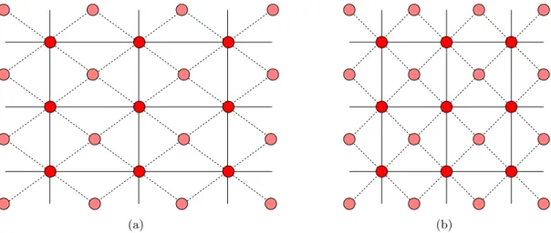
(a) (b)
Figure 2.1: Schematic illustration concerning lattice systems and Bravais lattice / basis.
– Mirror reflections along the lines parallel toa1 and a2, but not along diagonals
• Hexagonal lattice: ∣a1∣ = ∣a2∣ and angle between ⃗a1 and ⃗a2 is 60○. In addition to translational invariance, symmetry operations are
– Inversion symmetry through any lattice point
– Mirror reflections along the lines parallel toa1,a2, and a1−a2. – Sixfold rotational symmetry
• Oblique lattice: ∣a1∣ ≠ ∣a2∣and ⃗a1⋅ ⃗a2≠0. In addition to translational invariance, only inversion symmetry remains.
A lattice that one might see as a special oblique lattice is a rectangular lattice, where additional lattice points sit in the middle of each rectangle in addition to its corners. Since this lattice has all the symmetries of the rectangular lattice, see Fig.2.1(a), it belongs to the rectangular system rather than the oblique one. In 2D, the rectangular lattice system thus contains two Bravais lattices. In the square lattice, adding extra sites at the centers would also conserve all symmetries. However, one can here choose new basis vectors (⃗a1± ⃗a2)/2 and one then finds again a simple square lattice with a smaller unit cell, see Fig. 2.1(b).
Consequently, the square lattice system conatins only one Bravais lattice.
As a counter example, the honeycomb lattice is not a Bravais lattice: If we translate the lattice so that a lattice pointR⃗ comes to lie on the (former) position of its nearest neighbor, the lattice does not look the same as before. Mathematically, Eq. (2.4) cannot describe all lattice points. The honeycomb lattice can be obtained by putting a two-atom basis onto each lattice point of the hexagonal Bravais lattice. The atoms of a basis can also be of different kind, e.g., the differently shaded sites in Fig. 2.1 might be two different elements.
In that case, we would have a simple (rectangular or square) lattice with a two-atom basis.
2.2.2 Crystal lattices in 3D
Check out standard text books, e.g. Ashcroft-Mermin.
There are 7 lattice systems:
• Cubic: all angels 90○,∣⃗a1∣ = ∣⃗a2∣ = ∣⃗a3∣ Contains 3 Bravais lattices:
– Simple/primitive cubic
– Body-centered cubic: One site at the corner of a cube and one in its middle – Face-centered cubic: Additional sies at the centers of the cube’s faces
– (There is no “base centered cubic” lattice, because making one kind of cube faces special makes one of the three directions special and thus reduces the symmetry, so that this becomes a tetragonal lattice.)
• Tetragonal: all angels 90○,∣⃗a1∣ = ∣⃗a2∣≠∣⃗a3∣ Contains 2 Bravais lattices:
– Simple
– Body centered
– (There is no “base centered tetragonal” lattice either, because this is in fact a simple tetragonal one with a⃗1 and ⃗a2 rotated by 45○, similar to the case of Fig.2.1(a).)
– (By the same trick, “face centered tetragonal” is equivalent to “body centered”.)
• Orthorhombic: all angels 90○,∣⃗a1∣ ≠ ∣⃗a2∣ ≠ ∣⃗a3∣ Contains 4 Bravais lattices:
– Simple
– Body centered – Face centered
– Base centered: additional site in the center of the ‘floor’
• Monoclinic: one angle≠90○,∣⃗a1∣ ≠ ∣⃗a2∣ ≠ ∣⃗a3∣ Contains 2 Bravais lattices:
– Simple
– Base centered
• Rhombohedral: all angles equal, but ≠90○,∣⃗a1∣=∣⃗a2∣=∣⃗a3∣ (High-symmetry axes do here not run ∥ ⃗ai.)
• Hexagonal: two angle 90○, one 60circ,∣⃗a1∣ = ∣⃗a2∣ ≠ ∣⃗a3∣
• Triclinic: all angles ≠90○,∣⃗a1∣ ≠ ∣⃗a2∣ ≠ ∣⃗a3∣
There are thus 14 Bravais lattices. Together with a basis (e.g. diamond lattice), one can have additional symmetry operations.
As an example, the point group of the cubic system contains:
• 3 axes with 4-fold rotational symmetry,∥ ⃗a1,⃗a2,a⃗3
• 4 axes with 3-fold rotational symmetry, parallel diagonals through cube: ∥ ⃗a1+⃗a2+⃗a3,
⃗
a1− ⃗a2+ ⃗a3,−⃗a1+ ⃗a2+ ⃗a3,−⃗a1− ⃗a2+ ⃗a3
• 6 axes with 2-fold rotational symmetry, parallel diagonals of faces: ⃗a1± ⃗a2, ⃗a1± ⃗a3,
⃗ a2± ⃗a3
• Inversion
This is called the octahedral group with inversion symmetry Oh.
2.2.3 Unit cells
If repeated along the vectors a⃗i, a unit cell has to build up the complete lattice. This definition is not unique: One might always combine two unit cells into one, for example.
The face- and body-centered Bavais lattices are example where the ‘obvious’ unit cell contains more than one lattice site. As these are Bravais lattices, it is possible to define them with a one-site unit cell. One way to do this would be to use new vectors ⃗a′i obtained by connecting the site at the corner with its nearest neighbors (in the center of the adjacent cubes/faces). This would give a so-called ‘primitive’ unit cell with just one site, but would not reveal the symmetries as well.
A special primitive unit cell is the ‘Wigner-Seitz’ cell. The Wigner-Seitz cell around a lattice point R⃗ is given by all points that are closer toR⃗ than they are to any otherR⃗′. Its advantages are that it is primitive and has the proper symmetries, but its disadvantage is that its shape is often more complex.
2.3 Reciprocal Lattice
The aim of all the symmetry considerations is to make solving the Schr¨odinger equation easier, and the largest commutative (in order to be sure of having common eigenstates) group is the group of translations. As we know from math and from continuous translational invariance, Fourier transforms are coming in here, so we look at those. Check out a math text for Fourier transforms.
An important class of functions – and one where the topic of Fourier transforms immedi- ately suggests itself – are lattice periodic functions. Examples might be the potential seen by electrons moving in a perfect crystal. As the function is lattice periodic, we have
f(⃗x+ ⃗R) =f(⃗x) (2.5)
for any d-dimensional lattice vector R⃗ = ∑di=1nia⃗i. Assuming that it is sufficiently well behaved (which we do assume), it can be written as
f(⃗x) = 1
√Ω∑
G⃗
fG⃗e−iG⃗⃗x, (2.6)
where Ω= ⃗a1⋅ (⃗a2× ⃗a3)is the volume of a (not necessarily, but usually primitive) unit cell.
The ‘Fourier coefficients’ are obtained by fG⃗ = 1
√Ω∫
Ω
d3x f(⃗x)eiG⃗⃗x. (2.7) Note that various conventions exist concerning the signs in the exponential and the prefac- tors. For lattice periodic functions, the values ofG, for which⃗ fG⃗ ≠0 are restricted:
f(⃗x+ ⃗R) = 1
√Ω∑
G⃗
fG⃗e−iG⃗⃗xeiG⃗R⃗ =f(⃗x) ⇒ R⃗⋅ ⃗G=2πn (2.8) with integer n.
It turns out that allG⃗ fulfilling this form themselves a (Bravais) lattice, i.e., they can be expressed as
G⃗=∑d
i=1
mi⃗bi (2.9)
with integer mi. Furthermore, the basis vectors ⃗bi of this reciprocal lattice can be chosen to fulfill
⃗
ai⋅ ⃗bj =2πδij . (2.10)
It is straightforward to see that the relation (2.10) implies that G⃗R⃗=2πnis fulfilled:
G⃗R⃗=⎛
⎝∑
j
mj⃗bj⎞
⎠(∑
i
nin⃗i) = ∑
i,j
⃗bj⋅ ⃗ai
²=2πδij
nimj =2π∑
i
nimi
´¹¹¹¹¹¹¹¹¹¹¸¹¹¹¹¹¹¹¹¹¹¹¶
integer
(2.11)
It is maybe less obvious thatallvectorsG⃗fulfillingG⃗R⃗=2πncan be expressed by (2.9). We can show this by noting thatany reciprocal point (lattice or otherwise) can be expressed in terms of basis vectors⃗bi fulfilling (2.10) as long as we allow real coefficients αi. Out of all point, we now want to find all reciprocal pointsG⃗ with the property
1=eiG⃗⋅ ⃗R=exp(i(α1n1 a⃗1⃗b1
±2π
+α2n2a⃗2⃗b2+α3n3a⃗3⃗b3)) =e2πi(n1α1+n2α2+n2α2). (2.12)
Due to (2.10), all terms⃗bi⃗aj drop out fori≠j. Since this relationn1α1+n2α2+n2α2∈ Z has to hold for arbitrary integer ni, the alpha have themselves to be integer, i.e., any valid G⃗ has the form (2.9) and they consequently form a Bravais lattice. This lattice is in the same system as the direct-space lattice, but can be a different Bravais lattice. The reciprocal lattice of the body-centered cubic lattice, e.g., is the face-centered cubic lattice.
A possible of choice of basis vectors is
⃗b1=2π
Ωa⃗2× ⃗a3 (2.13)
⃗b2=2π
Ωa⃗3× ⃗a1 (2.14)
⃗b3=2π
Ωa⃗1× ⃗a2 (2.15)
or
bαi = π
Ωijkαβγaβjaγk (2.16)
with the Levi-Civita tensor andα,β,γ running through components x,y and z. Clearly
⃗
ai⋅ ⃗bj =0 for i≠j, because the cross product is orthogonal to each of its factors. For i=j, we get ⃗ai⋅ ⃗bi= 2πΩ⃗a1⋅ (⃗a2× ⃗a3) (or a cyclic permutation), yielding
⃗
ai⋅ ⃗bj =2πδij . (2.17)
2.3.1 Fourier transforms and Periodic Boundary Conditions (PBC)
While lattice-periodic functions are important, it would be too strong a restriction to only use those. What we do want to require is translational invariance. Lattice-periodic functions obey it, with eigenvalue 1, which is not necessary: other eigenvalues would also be fine. To motivate why we stick with Fourier transforms, though, note that exponentials of the form ei⃗kR⃗ have all the properties that (right) eigenvalues of the translation operator should have:
• As a symmetry operator, translations should be unitary, consequently, the absolute value of their eigenvalues should be 1. (Unitary operators are almost as nice as her- mitian ones when it comes to eigenvalues.)
• Combining two translations byR⃗1 andR⃗2 into one is possible (this is a group axiom) and we further know that this operation corresponds to a translation byR⃗1+ ⃗R2. This carries over to the eigenvalues of the common (as translations moreover commute) eigenvector: The product of the two eigenvalues ei⃗kR⃗1 ⋅ei⃗kR⃗2 is indeed the eigenvalue for the combined operation eik( ⃗⃗ R1+ ⃗R2).
• Similarly, the eigenvalue of the inverse element – translation by − ⃗R – works out:
(ei⃗kR⃗)−1=ei⃗k(− ⃗R).
• A note on the possible values ofk⃗labelling the eigenvalues: Adding a recoprocal-lattice point G⃗ leads to the same eigenvalues for all translations TR⃗i, because ei(⃗k+ ⃗G) ⃗Ri = ei⃗kR⃗ieiG) ⃗⃗ Ri =ei⃗kR⃗i . One can thus obtain all possible eigenvalues of the translations operators from ⃗k of a primitive unit cell of the reciprocal lattice; the first Brillouin zone.
• In a system with continuous translational invariance, the translation operator can be shown to be ˆT⃗r =eh̵ipˆ⃗rˆ⃗ for any r. The eigenvalues are then e⃗ i⃗kˆ⃗r, with h̵⃗k= ⃗p the (conserved) eigenvalue of the momentum operator. Here, only translations with lattice vectors R⃗ survive, but these should have analogous eigenvalues ei⃗kRˆ⃗.
The theory of Fourier transforms should consequently be helpful in understanding potential eigenfunctions.
It is customary to requestall physical quantities to be periodic with a much larger period than the lattice, this convention is called ‘periodic boundary conditions’. It is not necessary and sometimes not used, but it is useful. All functions are expected to fulfill
f(⃗x+ ∑
i
Nia⃗i) =f(⃗x), (2.18) whereNi≫1 is the lattice size along lattice vector⃗ai. In analogy to (2.8) and (2.9), looking at the Fourier transforms of such functions with larger periodicity gives
k⃗=∑d
i=1
mi Ni
⃗bi. (2.19)
The larger direct lattice thus allows much more finely spaced momentum points.
In fact, the primitive unit cell of the reciprocal lattice contains N1⋅N2⋅N3 momenta, as many points (and degrees of freedom) as there are lattice sites in the direct lattice. The primitive unit cell usually considered (but this is in principle arbitrary) in the case of the
reciprocal lattice is its Wigner-Seitz unit cell, it is termed the first Brillouin zone (1 BZ).
These momenta are ‘small’ compared to the points of the reciprocal lattice, but as there are as many as there are direct-lattice points, the degrees of freedom they can express are sufficient to express physics on ‘larger scales’, i.e., not looking into the unit cell.
We illustrate this with a few formulas: A special function that ‘cares only about the lattice sites’ is
f(⃗x) = ∑
R⃗
δ(⃗x+ ⃗R) (2.20)
with the delta-distribution ∫xdx δ(x−x0)f(x) = f(x0). This function is clearly lattice periodic, but can just as clearly not be used to express different functions within the unit cell. x⃗ can be anywhere in the full space, but as the sum runs over allR, we can also take⃗ it to be within the primitive unit cell around the closestR⃗ of the direct lattice. The Fourier transform (2.7) is
fG⃗ = 1
√Ω∫
Ω
d3x ∑
R⃗
δ(⃗x+ ⃗R)eiG⃗⃗x= 1
√Ω∫
Ω
d3x ∑
R⃗
´¹¹¹¹¹¹¹¹¹¹¹¹¹¹¹¹¹¹¹¹¸¹¹¹¹¹¹¹¹¹¹¹¹¹¹¹¹¹¹¹¹¹¶
∫all⃗x
δ(⃗x+ ⃗R)e−iG⃗R⃗
²=1
, (2.21)
where the sum oferR⃗ and the integral over Ω combine to give an integral over the full space R⃗+ ⃗x: R⃗ gives the large distances between lattice points and x⃗∈Ω the small ones within the unit cell. This becomes
fG⃗ = 1
√ΩeiG⃗R⃗ = 1
√Ω. (2.22)
Inserting this back into (2.6) gives an alternative expression off(⃗x)that must be the same as the original (2.20), i.e.:
∑
R⃗
δ(⃗x+ ⃗R) =f(⃗x) = 1 Ω∑
G⃗
eiG⃗⃗x (2.23)
We will use this equality to understand some aspects of Fourier transforms of functions that are not lattice periodic. They can be defined with respect to the large super lattice with volume V =N1N2N3Ω:
f(⃗x) = 1
√V ∑
all⃗k
f⃗ke−ik⃗⃗x= 1
√V ∫
q∈1BZ⃗
d3qe−iq⃗⃗x∑
G⃗
e−iG⃗⃗xfG+ ⃗⃗ q, (2.24)
where general momentumk⃗was decomposed into a ‘large’ partG⃗ that is a reciprocal lattice vector and a ‘small’ partq⃗from the first Brillouin zone. Let us now look at special functions f˜where ˜fG+ ⃗⃗ q is lattice periodic in the reciprocal lattice, i.e., ˜fG+ ⃗⃗ q=f˜q⃗. We then find using (2.23) that
f˜(⃗x) = 1
√V ∫
q∈1BZ⃗
d3qe−iq⃗⃗xf˜q⃗∑
G⃗
e−iG⃗⃗x= Ω
√V ∫
q∈1BZ⃗
d3qe−i⃗q⃗xf˜q⃗∑
R⃗
δ(⃗x+ ⃗R), (2.25)
which is only non-zero at lattice sites R. Such a function, which only depends on momenta⃗
⃗
q from the first Brillouin zone can thus not ‘see’ into the unit cell. However, this type of functions, where we are not concerned with the internal structure 1, are extremely com- mon in condensed-matter theory. In fact, it is often said that q⃗∈ 1BZ already describes
‘everything’.
These functions ˜f can also be written f˜(⃗x) =√
Ω∑
R⃗
f( ⃗R)δ(⃗x+ ⃗R) with (2.26) f˜( ⃗R) = 1
√N1N2N3∑
⃗q
f˜q⃗e−iq⃗R⃗ and (2.27) f˜q⃗= 1
√N1N2N3∑
R⃗
f( ⃗R)ei⃗qR⃗ . (2.28)
⃗
q runs here only over the first BZ, while R⃗ is a lattice vector of the direct lattice. Compare this to the equations (2.6) and (2.7) for lattice periodic functions, whereG⃗ is a (reciprocal) lattice vector andx⃗ runs only over the unit cell.
We can here note that direct-space vectors R⃗ indeed define the reciprocal lattice of the reciprocal latticeG⃗ and a few useful formulas should be noted:
∫
Ω
d3xei( ⃗G− ⃗G′) ⃗x=ΩδG,⃗G⃗′ and (2.29)
∫
ΩB
d3qei( ⃗R− ⃗R′) ⃗q=ΩBδR,⃗R⃗′ (2.30)
give orthonormality. ΩB = (2π)3/Ω is the volume of the first BZ and the integral over it should be understood to refer to very finely spaced q, i.e., a very large lattice, this limit is⃗ called the ‘thermodynamic limit’. Additionally,
Ω∑
R⃗
δ(⃗x+ ⃗R) = ∑
G⃗
eiG⃗⃗x and (2.31)
ΩB∑
G⃗
δ(⃗k+ ⃗G) = ∑
R⃗
ei⃗kR⃗ (2.32)
are useful.
The two special types of periodic functions that we discussed can be summarized as:
1Resp. take it into account in other ways.
Lattice periodic functions
• Defined for all positionsx.⃗
• Lattice periodic: f(⃗x) from primi- tive unit cell (=space between lattice pointsR) repeated to make full lattice:⃗ fx+ ⃗⃗ R=fx⃗; all unit cells equivalent.
• Only Fourier coefficientsfG⃗ ≠0 for re- ciprocal lattice vectorsG, see (2.9).
• Information on structure within unit cell.
• Identical for allR: Can’t describe vari-⃗ ations over more than one unit cell.
• Very useful for: lattice structure (Bra- vais lattice and basis within unit cell).
Functions periodic in reciprocal lattice
• Defined for all momenta ⃗kcompatible with PBC, see (2.19).
• fq⃗ from first BZ (=momenta be- tween reciprocal-lattice points G) re-⃗ peated to fill complete reciprocal lat- tice: f⃗q+ ⃗G=fq⃗; all BZs equivalent.
• In direct space, only f( ⃗R) ≠ 0 at lat- tice sites R.⃗
• Information on longer length scales be- yond unit cell.
• Only defined at Bravais-lattice siteR:⃗ Cannot look inside unit cell.
• Very useful for: excitations (e.g.
phonons, propagating electrons).
Both types of information are of course relevant, and in general, functions do not have to be periodic in either space, combining features from both sides. In the context of condensed- matter theory as treated in this class, functions periodic in G⃗ and defined only on lattice sites R⃗ are, however, going to be particularly important.
3 Separation of Lattice and Electrons and Lattice Dynamics
Inspired by Prof. Muramatsu’s and Prof. Valent´ı’s notes.
In this chapter, we want to discuss on a very qualitative level how solids are formed and then discuss in more detail excitations of the ionic lattice, i.e., phonons.
3.1 Adiabatic Approximation: Separate Hamiltonians for Electrons and Ions
A way to greatly simplify the problem of coupled ionic and electronic motion in Eq. (1.1) is partly decouple the electronic and lattice degrees of freedom. Atomic units are best suited to express the Hamiltonian, the unit of energy E0 is then the Hartree,E0 = meh̵24 = ea20 ≈27 eV, where the Bohr radius a0 = me̵h22 ≈ 0.5˚A makes a suitable unit of length. Position-space vectors r⃗and R⃗ are then expressed as r⃗=a0⃗r′, where ⃗r′ becomes a dimensionless number and is renamed ⃗r. This also changes the derivatives∂rα = a10∂r′α w.r.t componentα=x, y, z, which is again renamed to ∂rα. (And analogously for coordinates R⃗ of the nuclei.) In position space, the Hamiltonian (1.1) becomes
H E0 = −1
2∑
k,α
m Mk
∂2
∂R2k,α (3.1)
+1 2∑
k≠l
ZkZl
∣Rˆ⃗k−Rˆ⃗l∣ (3.2)
−1 2∑
i,α
∂2
∂r2i,α+1 2∑
i≠j
1
∣rˆ⃗i−ˆ⃗rj∣ (3.3)
− ∑
i,k
Zk
∣rˆ⃗i−Rˆ⃗k∣= (3.4)
=TN+Te+Ve+VN+Ve−N =TN+H0 (3.5) If the interaction Ve−N between electrons and nuclei, see (3.4), were small and if we could neglect it, this would decouple the two systems. Ifψ(⃗r) andφ( ⃗R)are the eigenstates of the electronic and ionic Hamiltonians, any product stateψ(⃗r)φ( ⃗R)would then be an eigenstate of the total Hamiltonian. However, the interaction term (3.4) is not smaller than the other terms and can certainly not be neglected: We know that the only the Coulomb interaction between electrons and nuclei allows the solid to form.
A term that is smaller than the others is thekinetic energyTN of the nuclei (3.1), which contains a factor Mm
k ≈ 10−5-10−4 and a first approximation consists of leaving it out. As
electrons are much lighter than ions, they move much faster and the assumption is that at any point during the ionic motion, the electrons have time enough to be in the instantaneous ground state, i.e., the electronic state depends only on the position of the nuclei at this time, but not on their momentum. When nuclei move (comparatively slowly), the electronic state can still change, as they react to the potential energy affected by the changed ionic positions.
But they remain in the ground state of the instantaneous ionic potential, such a process is called adiabatic, and the approach is therefore called adiabatic approximation.
The full Hamiltonian is thus divided into H0 (3.2-3.4) and the perturbation TN (3.1).
At first sight, this does not appear to help much, because H0 still contains terms referring to electrons and nuclei. However, the differential equation defined byH0 in position space does not contain derivaties w.r.t. nuclear coordinates R⃗ and these variables can thus seen as parameters, much like Zk or evena0. We then have a differential equation for eigenfunc- tions φα of the electrons, with operator H0 acting on this function and the corresponding coordinatesr.⃗
H0( ⃗R)φα(⃗r;R⃗) =α( ⃗R)φα(⃗r;R⃗) (3.6) Additionally, eigenvalues and eigenfunctions depend on parameters R⃗ and Zk. The ion-ion potential (3.2) is here just an additive constant (i.e. not affecting φ) that also depends on these parameters.
A first approximation can be to take0( ⃗R)andφ0(⃗r;R⃗)as electronic ground-state energy and ground state for given ionic positions R, if this is what one was interested in. One can⃗ then minimize the electronic ground-state energy 0( ⃗R) by varying positions R⃗ of the nu- clei. The resulting optimal positions should give a decent approximation to the equilibrium positions of the ions. As0( ⃗R)defines a potential for the nuclei (it also contains the ion-ion interaction) one can also us it to classically study motion of nuclei driven by this potential, an approach used in molecular-dynamics simulation.
3.1.1 Equilibrium Positions of the Ions: How the Lattice arises
The chemical processes actually stabilizing a solid are not a main point of this class, where we mostly assume it to exist. Nevertheless, a short summary of various types of bonding is useful, even though real materials usually lie between clear scenarios.
1. Van-der-Waals bonds: This type of bonds exists between neutral atoms or molecules, where a dipole moment can be induced by displacing the electronic cloud to one side. Even though the atom/molecule would by itself not have any dipole moment, it may be energetically favorable to create one once two such molecules become close to each other, because the interaction between the newly-created dipoles may gain more energy than the cost of the electron displacement. Dipole-dipole interactions are not as strong as, e.g., Coulomb interaction between ions and moreover fall off quickly with distance. The van-der-Waals interaction is∝r−6. However, it grows with the number of involved particles, to that it can in total become quite strong. For the same reason, it prefers dense packing.
An effective potential often used to model such a scenario is the Lennard-Jones po-
tential
VLJ(r) =4[(σ
r)12− (σ
r)6] . (3.7)
The second term is the van-der-Waals interaction, while the first term takes into account the fact that the atoms/molecules are repulsive on very short distances, i.e., they cannot sit on the same spot. 1 Forr/σ slightly larger than 1, it has a minimum, the equilibrium distance between two particles. This potential can be used to simulate the interplay of van-der-Waals interaction and kinetic energy.
2. Ionic bonds: In this case, two (or more) kinds of atoms (or molecules) are combined, the classic example is rock salt NaCl. Na has here one electron outside filled shells and Cl misses one. Since filled shells are energetically very stable, energy can be gained by transferring one electron from Na to Cl and since the atoms are then charge ions, Coulomb attraction comes into play. This Coulomb interaction between charge monopoles is strong compared to dipole-dipole interaction. It also profits from more ions being involved (suggesting dense packings), but they have to be mixed, which leads to some restrictions
3. Covalent bonding: Here, the electrons involved in the bondings are shared between two atoms and occupy common orbitals. Because of these orbitals, the bonds are quite directional and crystals may have quite a low packing density. The carbon-carbon bonds in diamond, which form tetrahedra, are a classic example.
4. Metallic bonding: When an element (e.g. Na) has electrons just outside filled shells, this electron can easily be moved away. As an s-electron of the next shell, its wave function can be quite large compared to the remaining ion and the range of its strongly repulsive short-distance interaction, and thus to the length scale of a plausible lattice constant. s orbitals of may atoms then see each other and due to their overlaps, electrons can easily move through the lattice and gain kinetic energy. This energy gain from partly filled bands stabilizes the solid.
5. Hydrogen bonds: Here, molecules (e.g. water) have a dipole moment (as opposed to the induced dipoles of the van-der-Waals interaction) due to the effective positive charge of the H atoms. The resulting interaction is almost close to a chemical bond.
3.1.2 Add back the kinetic energy of the ions
As a next step, we add back the kinetic energy of the ions and later decide which of the resulting terms to keep. To do so, we express the quantum mechanical state of the full system as ψ(⃗r,R⃗) = φ(⃗r;R⃗)χ( ⃗R), where we can expand the electronic partφ(⃗r;R⃗) in the eigenbasis of H0( ⃗R). As an eigenbasis is complete, any function can be expressed in this way, by using
φ(⃗r;R⃗) = ∑
α
cαφα(⃗r;R⃗). (3.8)
1Which can in turn be explained by the inner shells of the ions, or the nuclei, ‘seeing’ each other.
As the φα fulfill the eigenvalue equation (3.6), this gives 2 H0ψ(⃗r,R⃗) =H0∑
α
cαφα(⃗r;R⃗)χ( ⃗R) = ∑
α
cαα( ⃗R)φα(⃗r;R⃗)χ( ⃗R). (3.9) Applying the full Hamiltonian to this state ψ gives
Hψ= (H0+TN)ψ= ∑
α
cαα( ⃗R)φα(⃗r;R⃗)χ( ⃗R) −1 2∑
k,β
m Mk
∂2
∂R2k,βψ= (3.10)
= ∑
α
cα⎛
⎝α( ⃗R)χ( ⃗R) −1 2∑
k,β
m Mk
∂2χ( ⃗R)
∂R2k,β
⎞
⎠φα(⃗r;R⃗) (3.11)
−1 2∑
k,β
m Mk∑
α
cα
∂2φα
∂R2k,βχ− ∑
k,β
m Mk∑
α
cα
∂φα
∂Rk,β
∂χ
∂Rk,β = (3.12)
−1 2∑
k,β
m Mk∑
α
φα ∂2cα
∂R2k,βχ−1 2∑
k,β
m Mk∑
α
∂φα
∂Rk,β
∂cα
∂Rk,βχ− ∑
k,β
m Mk∑
α
φα ∂cα
∂Rk,β
∂χ
∂Rk,β =
=Eψ=E∑
α
cαφα(⃗r;R⃗)χ( ⃗R). (3.13)
Multiplying with the conjugate electronic ground state φ∗0 and integrating over all 3Ne
electronic coordinates r, i.e., taking a scalar product with⃗ ⟨φ0∣, yields E∑
α
cαχ( ⃗R) ∫ d3Ner φ∗0(⃗r;R⃗)φα(⃗r;R⃗)
´¹¹¹¹¹¹¹¹¹¹¹¹¹¹¹¹¹¹¹¹¹¹¹¹¹¹¹¹¹¹¹¹¹¹¹¹¹¹¹¹¹¹¹¹¹¹¹¹¹¹¹¹¹¹¹¹¹¹¹¹¹¹¹¹¹¹¹¹¹¹¹¹¹¹¹¹¹¹¹¹¹¹¹¸¹¹¹¹¹¹¹¹¹¹¹¹¹¹¹¹¹¹¹¹¹¹¹¹¹¹¹¹¹¹¹¹¹¹¹¹¹¹¹¹¹¹¹¹¹¹¹¹¹¹¹¹¹¹¹¹¹¹¹¹¹¹¹¹¹¹¹¹¹¹¹¹¹¹¹¹¹¹¹¹¹¹¹¹¶
=δα,0
= (3.14)
= ∑
α
cα
⎛
⎝α( ⃗R)χ( ⃗R) −1 2∑
k,β
m Mk
∂2χ( ⃗R)
∂R2k,β
⎞
⎠ ∫ d3Ner φ∗0(⃗r;R)φ⃗ α(⃗r;R)⃗
´¹¹¹¹¹¹¹¹¹¹¹¹¹¹¹¹¹¹¹¹¹¹¹¹¹¹¹¹¹¹¹¹¹¹¹¹¹¹¹¹¹¹¹¹¹¹¹¹¹¹¹¹¹¹¹¹¹¹¹¹¹¹¹¹¹¹¹¹¹¹¹¹¹¹¹¹¹¹¹¹¹¹¹¸¹¹¹¹¹¹¹¹¹¹¹¹¹¹¹¹¹¹¹¹¹¹¹¹¹¹¹¹¹¹¹¹¹¹¹¹¹¹¹¹¹¹¹¹¹¹¹¹¹¹¹¹¹¹¹¹¹¹¹¹¹¹¹¹¹¹¹¹¹¹¹¹¹¹¹¹¹¹¹¹¹¹¹¹¶
=δα,0
(3.15)
−1 2∑
k,β
m
Mkχ( ⃗R) ∑
α
cα∫ d3Ner φ∗0 ∂2φα
∂R2k,β (3.16)
− ∑
k,β
m Mk
∂χ
∂Rk,β∑
α
cα∫ d3Ner φ∗0 ∂φα
∂Rk,β (3.17)
−1 2∑
k,β
m Mk
∂2c0
∂Rk,β2 χ−1 2∑
k,β
m Mk∑
α
∂cα
∂Rk,βχ∫ d3Ner φ∗0 ∂φα
∂Rk,β − ∑
k,β
m Mk
∂c0
∂Rk,β
∂χ
∂Rk,β . (3.18) Assuming thatc0≈1≠0 and dividing by it, the first lines (3.14) and (3.15) give an eigenvalue equation for χ( ⃗R), with a kinetic energy TN,eff.and some potential 0( ⃗R):
⎛
⎝0( ⃗R) −1 2∑
k,β
m Mk
∂2
∂R2k,β
⎞
⎠χ( ⃗R) =Eχ( ⃗R). (3.19)
2Note that even for statescα=δα,0,ψ(⃗r,R⃗) =φ0(⃗r,R⃗)χ( ⃗R) is not strictly speaking an eigenstate ofH0, because the ‘eigenvalue’0( ⃗R)depends on R, which is a variable of⃗ ψ and not just some parameter, as it was forφ.
However, (3.17) mixes derivatives of φ and χ and couples thus the electronic and ionic kinetic energies. Additionally, (3.16) describes an operator that acts on the nuclear wave function with a weight given by derivatives of the electronic wave function, modifies thus both φ and χ and likewise undoes the decoupling. The adiabatic approximation neglects these terms, which is justified if they are ‘small’ compared to the terms included in H0 as well as compared to the nuclear motion (3.19). The energy scale of H0 is E0 = me̵h24. Eigenvalues of (3.19) will be discussed in detail in section 3.2, where energies hω̵ = ̵h
√K
M
of lattice vibrations are related to a ‘spring constant’ K that is in turn derived from the curvature of 0( ⃗R). Using a0=meh̵22 as a ‘typical’ unit of length, one estimates
∂2( ⃗R)
∂R2 ≈ E0 a20 = me4
h̵2 m2e4
h̵4 = m
h̵2E02 ⇒ ̵hω≈ ̵h
√K
M ≈√m
ME0. (3.20) Let us now compare the mixed terms to both electronic and ionic energy scales:
1. In estimating (3.16), it is useful to recall that the wave functionφ(⃗r;R⃗)knows aboutR⃗ only through the interaction Ve−N ∝ ∣ ⃗RZk
k−⃗r∣ between nuclei and electrons; the nuclear potential VN only changes the eigenvalue 0. The effect of the derivatives ∂/∂Rk,β should thus be approximately captured by ∂/∂ri,β. The integral in (3.16) thus turns out to be close to the kinetic energy of the electrons and of order E0. The full term is then of to order of Mm
kE0, or √m
M̵hω, i.e., smaller by a factor of 10−2-10−3 than the next smallest energy.
2. In the term (3.17), contributions forα=0 vanish for non-magnetic solutions φ. Such wave functions can be chosen realφ0=φ∗0 and the derivative∂/∂Rof the total density vanishes.
3. For α ≠ 0 and/or complex φ, we again approximate ∂φ/∂R by −∂φ/∂r. The two factors ∂χ/∂R and ∂φ/∂r are then the nuclear and electronic momenta. In atomic units⟨pel.⟩ ≈√
E0 and⟨pN⟩ ≈√
M
mhω, which leads together with the prefactor̵ Mm and hω̵ ≈√m
ME0 to the estimate
≈ m
M
√ E0M
m
√m
ME0= (m
M)3/4E0≈ (m
M)1/4̵hω . (3.21) While this is still smaller than the nuclear kinetic energy, (Mm)1/4 ≈10−1 -10−2, i.e., the difference is not very large considering how crude the estimates are.
Finally, the terms in (3.18) contains derivatives, i.e., they are relevant if the electrons care not always in the instantaneous ground state, i.e., for∂c0/∂R≠0. However, as perturbation theory tells us that such admixtures go withVl0/(El−E0)[withVl0the matrix element (3.21) connecting unperturbed eigenstates and(El−E0) ≈E0], these terms are indeed rather small.
The most important among the neglected terms, (3.17) which may not be so very small, is only non-zero when it involves different electronic eigenstates. In a perturbative treatment, energy differences α≠0−0 between these eigenstates enter in the denominator. The term can consequently more easily be neglected if electronic eigenstates are well separated. This is a different way of expressing the prerequisite for the adiabatic approximation, namely that electrons move so fast that they can alway stay in the ground state: When electronic