MPIfG Discussion Paper
One Currency and Many Modes of Wage Formation
Why the Eurozone Is Too Heterogeneous for the Euro
Martin Höpner and Mark Lutter
Max-Planck-Institut für Gesellschaftsforschung, Köln Max Planck Institute for the Study of Societies, Cologne August 2014
MPIfG Discussion Paper ISSN 0944-2073 (Print) ISSN 1864-4325 (Internet)
© 2014 by the authors
Martin Höpner is head of the Research Group on the Political Economy of European Integration at the Max Planck Institute for the Study of Societies, Cologne.
hoepner@mpifg.de
Mark Lutter is head of the Research Group on Transnational Diffusion of Innovation at the Max Planck Institute for the Study of Societies, Cologne.
lutter@mpifg.de
Downloads www.mpifg.de
Go to Publications / Discussion Papers
Max-Planck-Institut für Gesellschaftsforschung Max Planck Institute for the Study of Societies Paulstr. 3 | 50676 Cologne | Germany
Tel. +49 221 2767-0 Fax +49 221 2767-555 www.mpifg.de info@mpifg.de
Abstract
Synchronization of national price inflation is the crucial precondition for a well-func- tioning fixed exchange rate regime. Given the close relationship between wage inflation and price inflation, convergence of price inflation requires the synchronization of wage inflation. Why did the convergence of wage inflation fail during the first ten years of the euro? While differences in economic growth shape the inflation of labor costs, our argument is that the type of wage regime has an additional, independent impact. In coordinated labor market regimes, increases in nominal unit labor costs tended to fall below the ECB’s inflation target, while in uncoordinated labor regimes, the respective increases tended to exceed the European inflation target. To show this, we analyze data from 1999–2008 for twelve euro members. We estimate the increases of nominal unit labor costs both in the overall economy and in manufacturing as dependent variables, test a variety of labor- and wage-regime indicators, and control for a battery of eco- nomic, political, and institutional variables. Neither the transfer of wage coordination from the North to the South nor the transfer of adjustment pressure from the South to the North is likely to solve the problem of inner-European exchange-rate distortions.
Zusammenfassung
Die Synchronisation nationaler Inflationsraten ist die entscheidende Voraussetzung für ein funktionsfähiges Regime fester Wechselkurse. Wegen des engen Zusammenhangs zwischen Lohn- und Preisinflation ist hierfür eine Synchronisation der Steigerungen der Lohnstückkosten vonnöten. Warum kam während der ersten zehn Euro-Jahre keine Konvergenz der Lohnauftriebe zustande? Dies lag zum einen an den unterschiedlichen Wachstumsdynamiken der Euro-Teilnehmer, zum anderen an einem institutionellen Unterschied zwischen den Euro-Ländern: den Lohnregimen. In Ländern mit koordi- nierten Lohnregimen unterschritten die Steigerungen der Lohnstückkosten im Trend das Inflationsziel der Europäischen Zentralbank, in Ländern mit unkoordinierten Lohnregimen fielen die Lohnsteigerungen hingegen höher aus. Um dies zu zeigen, ana- lysieren wir Daten von zwölf Euro-Ländern für die Jahre 1999 bis 2008. Wir betrachten die nominalen Steigerungen der Lohnstückkosten sowohl gesamtwirtschaftlich als auch bezogen auf das verarbeitende Gewerbe und verwenden unterschiedliche Lohnregime- Indikatoren als erklärende Variablen. Zudem kontrollieren wir für zahlreiche ökono- mische, politische und institutionelle Kontextbedingungen. Weder eine etwaige Über- tragung der Lohnkoordination vom Norden auf den Süden noch eine Übertragung der ökonomischen Anpassungslast vom Süden auf den Norden scheinen geeignet, das Problem der innereuropäischen realen Wechselkursverzerrungen zu lösen.
Contents
1 Introduction: Desert racing without toolkits 1
2 A brief review of the debate 2
3 Applying the wage-bargaining literature to the Eurozone 5
4 Data and methods 8
5 Results 11
6 Conclusion: Choosing among bad options 18
Appendix 22 References 25
One Currency and Many Modes of Wage Formation:
Why the Eurozone Is Too Heterogeneous for the Euro
1 Introduction: Desert racing without toolkits
Entering a currency union is a risky bet. The potential gains are obvious. Currency unions eliminate the uncertainty of nominal exchange rates. This should stabilize the expectations of transnational economic actors, reduce their liquidity preference, and, as a consequence, increase their readiness to trade and invest. The more credible, reliable, and trustworthy the fixed exchange rate regime is, the more such effects should occur.
The most credible form of a fixed exchange rate regime is the currency union (de Grau- we 2012: 105–113). However, currency unions eliminate not only the uncertainty about nominal exchange rates, but also the availability of nominal exchange rate adjustments as a decisive macroeconomic policy tool. Member states cannot use nominal devalua- tions and revaluations as adjustment tools once inflation divergences occur. The crucial precondition for a well-functioning currency union is, therefore, the capacity to syn- chronize price inflation.1 Given the close relationship between the inflation of nominal unit labor costs (hereafter: NULC) and price inflation, synchronization of price inflation in turn presupposes synchronization of NULC inflation. Yet, if NULC developments diverge over a longer period of time, the fact that economic actors have been freed from the uncertainties of nominal exchange rates becomes a problem. Entering a currency union is like a jeep race through the desert in which teams leave their toolkits behind in order to make their cars as light as possible – in the hope that the toolkits will not be needed anyway.
The euro crisis indicates that the Eurozone has lost this bet. Since the introduction of the euro in 1999, substantial differences have arisen with regard to NULC inflation and price inflation, with Austria and Germany positioned at the stagnating end of the scale and the Southern economies positioned at the inflating end. In the context of these distortions of the real exchange rate, the nonavailability of the nominal de- and re-
We thank Lena Ehret for research assistance and Lothar Krempel, Florian Rödl, Fritz W. Scharpf, Armin Schäfer, and Annika Wederhake for helpful comments.
1 This is why the national inflation preference figured prominently in Fleming’s theory of opti- mal currency areas. Interestingly with regard to the argument in this paper, Fleming noted that
“particular importance attaches to the degree of co-ordination or unification that exists among the trade union and employers’ organisations that are active in the various countries of the fixed exchange rate area. So long as these bodies are organised on a purely national basis, and so long as moods and motivations affecting the workers are different and change differently in different countries, there will probably arise shifts and divergencies in relative labour costs which will require for their correction adjustments in relative exchange rates” (Fleming 1971: 477).
valuation tool has indeed become a problem.2,3 In 2012, for example, a Goldman Sachs study indicated that the German economy needed a revaluation of about 25 percent and the Portuguese economy a devaluation of about 35 percent, with all other euro members positioned in between these two extremes.4 If the option of adjusting the nominal exchange rate had been available since the mid-2000s, it would have undoubt- edly been used. However, since the nominal exchange rate was fixed, euro countries had to choose between ignoring distortions of the real exchange rate (a bad choice because of the immediate consequences for trade and indebtedness and the medium- to long- term consequences for interregional economic development) and pushing overvalued economies towards internal devaluations (another bad choice because the adverse so- cial consequences made it rather unlikely that democratically elected politicians would agree on the respective strategy).5 We all know what then happened. This study sheds light on why the bet was lost in the first place, thereby highlighting the political-eco- nomic heterogeneity of the Eurozone and, in particular, the heterogeneity of European labor and wage-bargaining regimes.
2 A brief review of the debate
In 2012, Lo wrote a fascinating literature review on the emergence of the financial crisis.
He read and reviewed 21 books and came to the conclusion that they offered no less than 21 different causal narratives (Lo 2012). The situation is not very different when we turn to the euro crisis. A variety of causal interpretations coexist, and, although dif- ferent, they each possess internal plausibility. In order to clarify our starting point and our contribution, we will concentrate in the following not on the differences, but on the common core within one particular strand of the literature: the strand that inter- prets the euro crisis not mainly as an outcome of irresponsible budget policies of cer- tain European governments, but as a symptom of deeper macroeconomic imbalances.
2 See Johnston/Regan (2014), who show that inflation’s impact on the current account is condi- tional on the exchange rate regime.
3 Regionally heterogeneous price developments exist in other common currency areas as well, such as the United States. A unique European problem was, however, the persistence of inflation divergences. In the US, inflation differences of more than one percentage point rarely persist longer than two years. During the first ten Eurozone years, in contrast, the very same countries remained on the upper and on the lower ends of the inflation scale. See European Central Bank (2005: 62–63; 2012: 71).
4 See the details in Sinn (2014a: 120). The most alarming finding of that study was the devalua- tion need of about 20 percent in the case of France.
5 See our conclusion, in which we also discuss reflation in the North as an alternative to deflation in the South.
Notwithstanding emphases on different parts of the causal narrative, it is fair to argue that many political-economy narratives on the euro crisis agree on the following causal building blocks, or at least on most of them.6
In Southern Europe, the euro facilitated the availability of cheap credit for two reasons:
risk premia on government bonds declined because the risk linked to the nominal ex- change rate was eliminated, and ex ante higher inflation rates led to dysfunctionally low real interest rates. Regardless of whether debt was mainly issued by the state (as in Greece) or by private actors (as in Spain), the result was a debt-driven boom in which trade deficits and current account deficits rose. Again, that happened for two reasons:
first, rising demand led to rising imports; second, due to rising wages, the respective countries forfeited competitive strength.7 In 2008, triggered by the Lehman crisis, capi- tal markets began to doubt the ability of Southern countries to finance their current ac- count deficits. Note that, in this account, the debt crisis is a causally subordinated – but nevertheless disastrous – effect of distorted real exchange rates, rather than the ultimate cause of the current problems.8
Even more succinctly put, the common core reads: cheap credit growth NULC inflation price inflation competitive disadvantage current account deficit debt crisis.9 While we agree with the essence of this account, we will show in the following that substantially more variance can be explained by making the narrative only slightly more complicated. We concentrate on the causes of heterogeneous NULC increases. While our data will confirm that growth differentials have indeed (and unsur- prisingly) contributed to the divergences in NULC inflation, we will show that a par- ticular form of institutional differences had an independent effect on NULC inflation, too: the heterogeneity of inner-European labor and wage-bargaining regimes. This point has consequences for the prospects of convergence in the Eurozone. Due to the stickiness of labor regime institutions, the Eurozone’s inability to synchronize inflation is not likely to be remedied in the foreseeable future. Therefore, we have reason to be-
6 For example, parts of this “emerging consensus” are to be found in Collignon (2013); Flassbeck/
Lapavitsas (2013: chap. 2); Giavazzi/Spaventa (2011); Hall (2012); Jones (2011: 291–299); Krug- man (2011a); Scharpf (2013: section 2; 2014: section 2); Sinn (2014: chaps. 2–4 and 8; 2014:
sections 2–4).
7 The very reverse happened in Northern Europe, especially in Germany: Germany had an ex ante low inflation rate, was therefore confronted with a dysfunctionally high real interest rate, and did not profit from the risk premia convergence of government bonds. It accumulated current account surpluses for two reasons: first, the lack of internal demand led to low imports; second, due to low NULC increases, Germany’s goods gained a competitive cost advantage.
8 This stands in contrast to large parts of the public debate in the countries of the former deutsch- mark bloc, which claim that the crisis was caused mainly by unsound budget policies in South- ern Europe. A fine example is Wirtschaftsrat Deutschland (2011).
9 Note that another causal arrow goes directly from growth to the trade deficit (because of the hunger for imports in the boom countries and the lack of a respective hunger in the stagnation countries). For the emergence of trade balances, credit-driven Southern imports were no less important than the overvaluation-driven lack of exports.
lieve that the Eurozone will continue to have a structurally determined need for the toolkit that we mentioned in the introduction – flexibility in nominal exchange rates – and that the Eurozone may have to pay a significant price for having left it behind.
By emphasizing the role of wage bargaining, we confirm a point that has been made by Collignon (2009), Höpner (2013), Ramskogler (2013), and, in particular, Hancké and colleagues (Hancké 2013a and b; Johnston 2012; Johnston/Hancké/Pant 2013). To date, Hancké’s book (2013a) is the most elaborated account of how wage-bargaining regimes shaped the macroeconomic imbalances in the Eurozone.10 He argues that two different logics applied in the exposed and the sheltered sectors of Eurozone countries.
In the exposed sectors, international market pressures had sufficient power to contain high wage demands. Therefore, exposed-sector NULC remained more or less stable in all Eurozone countries. But in the sheltered sectors, especially in the public sectors, in- ternational market pressures were absent. Whether or not wage restraint in exposed sectors could be transmitted to the rest of the national economy depended on the over- all coordination of the wage-bargaining system.11 As a consequence, wage increases in sheltered and exposed sectors remained in line in the coordinated economies but fell apart in the countries with uncoordinated wage-bargaining systems.
According to Hancké’s narrative, the regime type should mainly affect in the sheltered sector, but not in the internationally exposed sector. For a number of reasons, we won- der whether theoretical reasoning justifies this expectation:
1. Exposed-sector employees may have an interest in nominal disinflation vis-à-vis trading partners (not to be confused with an interest in real wage losses) which em- ployees in the sheltered sector lack. But this interest is collective in kind, rather than individual. Imagine an economy that is entirely exposed. All insights of the corporat- ism literature (which we will discuss in detail in Section 3) still apply: Collectively, all employees might profit from holding down NULC; individually, it is another story.
Once individual workforces expect other wage bargainers to engage in inflationary wage settlements, it becomes irrational to stick to the collective interest. In other words, even the exposed sector should require a coordination tool to bring about NULC restraint.
2. Even if we assume that rising firm-level NULC directly translate into job losses in the respective firm, the coordination problem does not vanish entirely. If trade unions are divided along ideological lines, the collective action dilemma reoccurs at the firm level. If we assume that NULC disinflation is unpopular, at least in the short run, then restraining nominal wage demands will be irrational in such a situation.
10 See also the debate on Hancké’s book in an upcoming issue of Labor History.
11 In uncoordinated wage-bargaining regimes, the sheltered sector has a “natural” leading func- tion due to its larger size. Therefore, it is wage coordination that determines whether the leading role can be shifted from the sheltered to the exposed sector.
3. Consider now what is likely to happen if exposed-sector unions overcome their co- ordination dilemma but fail to transmit NULC restraint to the rest of the economy.
Assume again that their preference for NULC deflation does not imply a preference for real wage loss. In such a situation, exposed-sector unions must choose between two undesired outcomes: real wage losses and losses in competitiveness. Since we have no reason to believe that export unions will choose competitiveness entirely at the expense of real wage losses, we should assume that they partially converge to the wage policies of the nonexposed sector. Again, this leads us to expect the amount of wage coordination to matter not only for the overall economy, but also for the exposed sector.
In this paper, we will analyze data from twelve euro countries in order to shed light on the determinants of NULC developments during the first ten euro years (until the start of the financial crisis). We will look at both economy-wide developments and the manufacturing sector (serving as a proxy for the exposed sector). In accordance with Hancké (2013a), we will confirm that NULC increases in manufacturing were indeed lower than the respective increases in the overall economy. Interestingly, the variance of nominal wage pressure was higher, rather than lower, in manufacturing than it was in the overall economy. In other words, we do not find the convergence of NULC increases in the exposed sectors that we might expect with respect to Hanckés narrative; instead we find unexpected amounts of variance. Applying regression techniques and a variety of wage-coordination indicators and numerous controls, we will show that wage coor- dination shapes NULC both economy-wide and in manufacturing, irrespective of the actual wage-coordination indicator chosen.
Before we turn to the quantitative part of our study, we revisit the wage-bargaining literature in more detail and discuss whether its insights are still likely to apply to fixed exchange rate regimes.
3 Applying the wage-bargaining literature to the Eurozone
The main insight of the comparative literature on wage bargaining is that the capacity to perform wage restraint is endogenous to the degree of coordination in the system of labor relations. If wage bargaining takes place in a decentralized and uncoordinated manner (i.e., each unit bargains on its own), then each unit has to be concerned about the inflationary wage deals of other units. Therefore, it is rational to add an anticipated inflation surplus to one’s own wage demand. If this happens in every unit, anticipated inflation does actually occur. However, uncertainty about the wage deals of other units
disappears if wage bargaining is coordinated (through centralization or horizontal sig- naling). Nominal wage pressures are thus likely to vary inversely with the degree of coordination in wage bargaining.12
So far, our review of the wage-bargaining literature has focused on a particular dys- function of uncoordinated wage-bargaining regimes (the anticipated inflation surplus) without taking into consideration the strategic capacities of coordinated wage bargain- ing. Since the late 1990s, however, the debate on comparative wage bargaining has con- centrated on the institutional preconditions that allow wage bargainers to act strategi- cally and to take into account the moves of other macroeconomic “players.” This is most evident in the literature on the interaction between wage and monetary policy, which argues that conservative central banks work better in interaction with coordinated wage bargaining. Only if wage bargaining is coordinated can central banks impose wage re- straint by simply threatening to impose higher interest rates (Hall/Franzese 1998; Sos- kice/Iversen 1998). The decisive point for our analysis is that this literature ascribes a certain capacity for long-term, foresighted, strategic action to coordinated wage bar- gainers, a capacity that uncoordinated wage bargainers lack.
Yet another insight into the preconditions and functions of coordinated wage bar- gaining comes from the comparative literature on production regimes (Streeck 1991;
Hall/Soskice 2001). This literature theorizes the interaction of production-related in- stitutions. For example, strategic wage restraint may become possible not only when wage bargaining is coordinated, but also when employees are institutionally protected against dismissals and when employers grant codetermination rights to employees.
Both features should provide employees with a long-term perspective inside the firm and should therefore encourage forms of strategic cooperation that pay off only in the medium run. If this holds true, the institutions of wage bargaining, layoff protection, and codetermination are – in the language of production regime theorists – function- ally complementary. The decisive point for our analysis is that this insight shifted the focus from the coordination capacity of isolated institutions to the overall coordination of entire production regimes (Hall/Gingerich 2004).
Let us now consider whether the insights discussed above should apply to the Euro- zone. To begin with, the heterogeneity of wage-bargaining regimes has not vanished in the ongoing process of European integration, neither in the EU-28 nor in the Euro- zone-18 (Höpner/Schäfer 2012: section 3). Labor relations in Europe differ with respect to a multitude of dimensions. Among them are membership levels in trade unions and 12 See the overviews provided in Kenworthy (2002) and Streeck/Kenworthy (2005). Hancké (2013:
100) notes that coordination may also depress NULC through another channel: coordination leads to wage compression, wage compression increases incentives to push productivity, and productivity is the denominator of the NULC calculation. However, the time period we ob- served was one in which wage compression declined everywhere, also (and in particular) in countries with moderate NULC increases, such as Germany (where NULC actually even slightly declined; see Section 4).
employers’ associations, organizational degrees of fragmentation along political and profession lines, the presence and “encompassingness” of central collective agreements, vertical centralization and horizontal signaling, state intervention in wage bargaining, minimum wages, and inflation indexation, just to mention a few (Du Caju et al. 2008).
It is fair to conclude that the capacity to avoid uncertainty about the inflationary wage deals of other bargaining unions – and the resulting capacity to abstain from anticipa- tory inflation surpluses – should be unevenly distributed across the Eurozone.
As we have seen above, a strand of literature has additionally ascribed a certain capabil- ity for long-term oriented, strategic wage policy to coordinated wage bargaining. Does the capacity to exert strategic wage restraint remain in place under conditions of fixed exchange rates? For two reasons, we argue that such a capacity should be even more pronounced when the exchange rate is fixed. Let us first imagine an exposed-sector trade union in a flexible exchange rate regime, and let us suppose that this trade union has the choice between a wage policy that is in line with advances in productivity and a strategy of wage moderation. We assume that the latter strategy has the disadvantage of being unpopular among members, at least in the short run, but it may depress export prices, generate trade surpluses, back up export-sector job security, and perhaps estab- lish a basis for higher wages in the future. In such a situation, the export-sector union should be reluctant to consider the unpopular choice, because trade partners may de- valuate their currency and therefore thwart the social partners’ moderation strategy.
In other words, under conditions of flexible exchange rates, even exposed-sector trade unions will tend to choose their strategies mainly – or at least to a significant extent – with an eye to the domestic economy.
But what happens if the exchange rate regime shifts? If trade partners cannot devaluate, it becomes more likely that nominal wage restraint will actually result in the enhance- ment of price competitiveness not only in the short, but also in the medium run. Ac- cession to a fixed currency regime should, therefore, gradually alter the relative weight of considerations upon which exposed-sector trade unions base their wage demands.
Another mechanism can be expected to lead to a similar effect: the nonavailability of alternative macroeconomic adjustment tools. If we consider the fiscal pact as a part of the euro regime, three of the four macroeconomic policy instruments usually available become inaccessible: interest rate policies, exchange rate policies, and fiscal policies.
What remains is the option of stimulating the economy through the export channel, that is, of entering into transnational wage competition (see also Hancké 2013a: chap.
3). However, it will depend on the structure of the wage-bargaining regime whether this tool is available in practice or in theory only. We conclude that there is no reason to believe that wage coordination will forfeit its functional significance under conditions of fixed exchange rates.
4 Data and methods
Dependent variables and points of observation
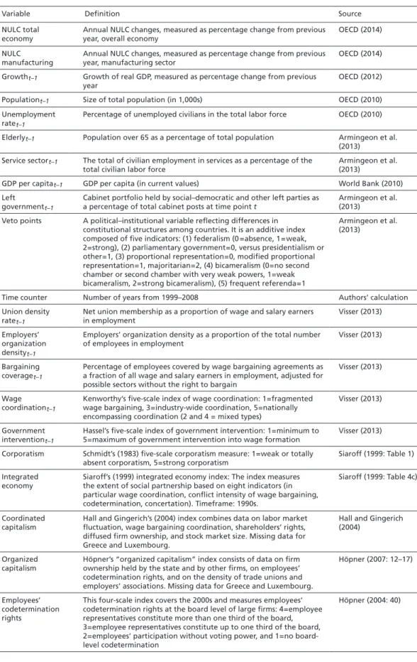
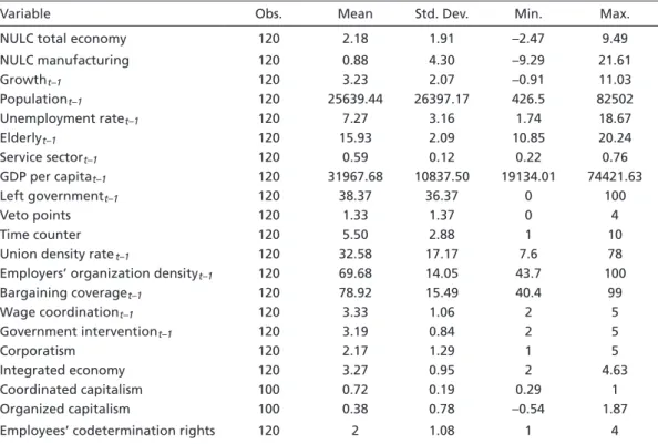
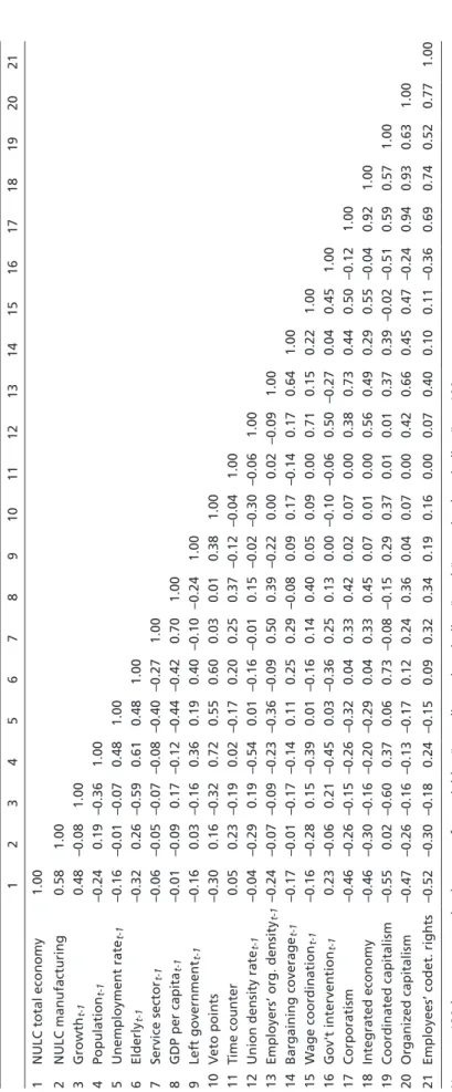
We will test whether the heterogeneity of European labor and wage-bargaining regimes contributed to the NULC divergences that emerged during the first ten euro years. For this purpose, we analyze yearly data from the eleven countries that introduced the euro as deposit money in 1999 and as hard cash in 2002, plus Greece, which joined the Eu- rozone in 2001.13 Our last year of investigation is 2008 due to the unfolding of the financial and the euro crises and the emergence of the Troika regime in the subsequent years. In other words, we analyze the “normal” operation of the Eurozone rather than the crisis regime (but see the concluding section). Our dependent variables are annual NULC changes (percentage change from previous year) in the overall economy and in the manufacturing sector, the latter serving as a proxy for the exposed sector (data source: OECD 2014).14,15 The appendix provides tables with definitions and sources (Table A1), summary statistics (Table A2), and a correlation matrix (Table A3) of all dependent and independent variables used in this study.
Independent variables
Our substantial independent variables shall test whether the wage regime hypothesis sheds light on the part of the NULC variance that remains unexplained by variance in growth. Rather than just showing results for one wage-regime variable, we will sepa- rately test a set of ten variables which, in different ways and from different theoretical angles, cover features of European wage bargaining, labor relations, and production regimes. The variables can be divided into five groups (see also Table A1).
13 Thus, the twelve countries we analyze are Austria, Belgium, Finland, France, Germany, Greece, Ireland, Italy, Luxembourg, the Netherlands, Portugal, and Spain.
14 Sadly it is not possible to construct a meaningful NULC measure for the sheltered sector be- cause data is lacking for its most important component, the public sector (to which Hancké and colleagues refer in their comparison of sheltered and exposed sector dynamics). NULC for the public sector cannot be calculated because information on the denominator of NULC, produc- tivity, is lacking (or better: not even defined).
15 Specifically, we use quarterly benchmarked and seasonally adjusted NULC since these values provide better estimates than do the nonadjusted variants. For the overall economy, however, adjusted values are missing for Portugal and Greece. We use the nonadjusted variant for these countries as an estimate. An alternative proxy for the internationally exposed sector in the in- ternational statistics is “industry,” which encompasses not only manufacturing but also mining and quarrying, as well as electricity, gas, and water supply (C, D and E in Revision 3.0 of the International Standard Industrial Classification, ISIC). We also tested this alternative proxy, and received the same results concerning our substantial variables (results are available from the authors).
1. The first three variables are not constructed indices but direct measures of features of the national wage-bargaining regimes. The variables are defined as (1) union density rate, in percent (net union membership as a proportion of wage and salary earners in employment); (2) employers’ organization density, defined as the net percentage of employees whose employers are members of their respective associations; (3) bar- gaining coverage, in percent, which is the percentage of employees covered by wage- bargaining agreements as a fraction of all wage and salary earners in employment, adjusted for possible sectors without the right to bargain. All three variables vary over time. Missing years have been interpolated from given years per country. The data source is the latest version of the ICTWSS database, version 4.0 (Visser 2013).
2. This group consists of two time-varying variables on the modes of wage forma- tion. The first is an index on wage coordination, initially constructed by Kenworthy (2001). 1 stands for fragmented wage bargaining, 3 for industry-wide coordination, and 5 for nationally encompassing coordination (with 2 and 4 being mixed types).
The second is an index on government intervention in wage bargaining, initially con- structed by Hassel (2006: chap. 3). This index has five ranks as well. 1 stands for a minimum and 5 for a maximum of government intervention into wage formation.
The data source is again Visser’s (2013) latest ICTWSS database (version 4.0).
3. The third group consists of two “classical” corporatism indicators, constructed for time periods before the euro. The first is Schmidt’s (1983) corporatism measure, which applies to the 1970s and early 1980s. The measure takes the value 5 for coun- tries with strong corporatism and 1 for weak or totally absent corporatism (data source: Siaroff 1999: table 1). The second is Siaroff ’s integrated economy index. It covers the 1990s and measures the extent of social partnership in a multitude of spheres (in particular, wage coordination, conflict intensity of wage bargaining, co- determination, and concertation). The data source is Siaroff (1999: table 4c).
4. The next two variables relate to the “varieties of capitalism” school and measure coordination not only in the labor relations sphere, but also in the corporate gover- nance sphere. Both indicators cover 1990s data and have missing data for Greece and Luxembourg. Hall and Gingerich’s coordinated capitalism index combines data on labor market fluctuation, wage-bargaining coordination, shareholders’ rights, dif- fused firm ownership, and stock market size (source: Hall/Gingerich 2004: 10–17).
Höpner’s organized capitalism index consists of data on firm ownership held by the state and by other firms, on employees’ codetermination rights, and on the density of trade unions and employers’ associations (source: Höpner 2007: 12–17).
5. The last variable covers the extent of employees’ codetermination rights at the board level of large firms and serves as a proxy for firm-based productivity coalitions (i.e., coordination at the company level). This index covers the 2000s. 4 stands for em- ployee representatives constituting more than one third of the board, 3 for employee representatives constituting up to one third of the board, 2 for employees’ participa-
tion without voting power, and 1 for no board-level codetermination (this index was first published in Höpner 2004: 40).
Controls
In addition to these predictor variables, we use growth of real GDP (measured as per- centage change from the previous year) as the main alternative predictor variable (see Section 2). The data source is OECD (2012). In order to rule out other possible influ- ences on the dependent variable, we include a battery of control variables. These include controls for possible (1) sociodemographic, (2) economic, (3) political, and (4) time- trend effects.
1. Four sociodemographic variables control for possible effects caused by country dif- ferences in population size, unemployment, and demographic and sectoral charac- teristics that might impact NULC changes: Population is the size of the total popula- tion (in thousands). The data source is OECD (2010). Unemployment rate is the per- centage of unemployed civilians in the total labor force. The source is OECD (2010).
Elderly is the population over the age of 65 as a percentage of total population. The data source is the Comparative Political Data Set I, compiled by Armingeon et al.
(2013). Service sector is the total number of people working in the service sector of civilian employment as a percentage of the total civilian labor force. Once again, the data source is Armingeon et al. (2013).
2. In addition to GDP growth, the models include GDP per capita (measured in current values). GDP per capita controls for effects on NULC increases due to different eco- nomic productivity levels among countries. The data source is World Bank (2010).
3. Two political control variables aim to rule out possible effects due to differences in political-institutional configurations, as well as in the party composition of the gov- ernment: Left government is the cabinet portfolio held by social-democratic and oth- er left parties as a percentage of total cabinet posts at time point t. The data source is Armingeon et al. (2013). Veto points are a common political-institutional con- trol variable reflecting differences in constitutional structures among countries. It is an additive index composed of five indicators: (1) federalism (0=absence, 1=weak, 2=strong); (2) parliamentary government=0, versus presidentialism or other=1; (3) proportional representation=0, modified proportional representation=1, majoritar- ian=2; (4) bicameralism (0=no second chamber or second chamber with very weak powers, 1=weak bicameralism, 2=strong bicameralism); (5) frequent referenda=1.
The data source is again Armingeon et al. (2013).
4. Time trend: We include a time counter (number of years from 1999–2008) in order to capture possible unobserved heterogeneity due to time trends affecting both the dependent and independent variables.16
Analytical approach
Our country-year panel dataset has a pooled time-series cross-section structure with the yearly data of twelve countries between 1999 and 2008. In order to account for a possible simultaneity bias, all time-varying independent variables are lagged by one year (Beck/Gleditsch/Beardsley 2006: 28). Since the dependent variable has a clear met- ric scale and can take negative as well as positive values, linear panel regression is the appropriate specification technique. Specifically, we fit random-effects regression with cluster-robust standard errors (clustered by countries) in order to account for coun- try-wise heteroscedasticity and possible violations of independence assumption (Beck/
Katz 1995). The random-effects model (rather than a fixed-effects approach) is appro- priate for the following reasons (Cameron/Trivedi 2010: 235–63): first, it provides a more efficient estimation technique than do the regular pooled OLS estimator, related variants of the population-averaged approach, or the pure “between” model. Second, it allows the estimation of time-invariant covariates. Since some of our main predic- tor variables do not change over time and others vary only slightly with time, a fixed- effects approach is unidentifiable or misleading for those variables. Moreover, from our theoretical perspective, a random-effects approach is the appropriate tool because we have empirical and theoretical reasons to assume that coordination regimes are rather
“sticky” and do not change substantially across time. Hence, a random-effects approach is a good compromise and allows us to estimate how differences between countries re- garding their types of coordination regimes affect differences between countries’ NULC changes, while providing an estimate of the possible overall within-explanation as well.
5 Results
Before we turn to the results of the regression analysis, let us explain the overall struc- ture of our dependent variables, our most important control variable (growth), and a number of variables that are causally downstream from our dependent variables (but which will not be subject to the subsequent regression analysis; data source: OECD).
Table 1 displays the cumulated changes of NULC (economy-wide and manufacturing), growth, and inflation over our period of observation, 1999–2008 (the variables are or- 16 In a previous analysis, we used quadratic and cubic transformations of time (t, t2, and t3). Results
were essentially the same as those presented here (available upon request).
dered with respect to the causal narrative in Section 2: cheap credit growth NULC inflation price inflation competitive disadvantage current account deficit debt crisis). We first look at the cumulated economy-wide NULC changes.
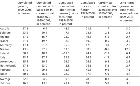
Between 1999 and 2008, and taking all countries in our sample into account, NULC rose by 24.5 percent. If we interpret the ECB’s 2-percent price inflation target as an im- plicit wage inflation target, it turns out that, on average, things worked pretty well dur- ing the first ten euro years: +24.5 percent is not far away from the +21.9 percent to which a yearly rise of 2.0 percent cumulates after ten years. However, the average hides huge variance. In Germany and Austria, NULC remained more or less stable, while NULC rose by almost 30 percent in Portugal and about 36 to 49 percent in Greece, Ire- land, and Spain – which are precisely the countries, besides Cyprus (not in our sample because it only introduced the euro later), that had to join the euro rescue fund. The average deviation from the average 24.5 percent NULC increase is +/–13.8 percentage points. The two countries closest to the average (and therefore to the ECB target) are France and Belgium. With respect to their NULC increases, they behaved comme il faut.17 Let us move on by comparing this information to the NULC changes in manufactur- ing. In this sector, NULC rose more moderately than in the overall economy (by 9.6%).
This clearly confirms the point made by Hancké and his colleagues: it was not the ex- posed sectors but the sheltered sectors that were the main drivers of nominal wage pressure (Hancké 2013a). However, interestingly, the variance behind this average was 17 Note in this context that German NULC changes were farther away from the inflation target than the respective changes of all other countries, including Portugal, Greece, Spain, and Ireland.
Table 1 Overview of selected variables Cumulated
growth, 1999–2008, in percent
Cumulated nominal unit labor cost in
creases (total economy), 1999–2008, in percent
Cumulated nominal unit labor cost in
creases (manu
facturing), 1999–2008, in percent
Cumulated price in
flation, 1999–2008, in percent
Current ac
count surplus, averaged over 1999–2008, in percent
Long–term government bond yields, averaged over 2009–2013, in percent
Austria 27.2 6.4 –8.2 21.9 1.7 3.0
Belgium 23.9 20.4 7.1 24.6 2.8 3.3
Finland 37.5 16.7 –23.0 19.8 5.5 2.7
France 21.4 19.7 2.3 19.0 0.5 3.0
Germany 17.1 –1.8 –5.0 17.3 3.0 2.3
Greece 43.6 37.5 53.0 38.3 –8.6 12.5
Ireland 68.8 48.9 –11.0 44.7 –2.1 6.1
Italy 13.4 27.9 29.8 26.3 –1.2 4.7
Luxembourg 55.6 29.4 26.2 26.9 9.8 2.2
Netherlands 27.1 23.0 2.8 24.6 5.2 2.7
Portugal 17.0 29.8 13.1 45.5 –9.6 7.3
Spain 40.4 36.3 28.2 37.3 –5.9 4.8
Average 32.8 24.5 9.6 28.9 0.1 4.6
Std. dev. 16.9 13.8 21.4 10.0 5.9 3.0
Note: Authors’ own calculations from OECD sources.
not smaller than in the overall economy; in fact, it was larger, even though all of these sectors were equally exposed to international competition. The average deviation from the mean of +9.6 percent was +/–21.4 percentage points (but note that the variance is partly driven by one outlier, Greece). It should not surprise us that, despite these differ- ences, the cumulated NULC changes in the overall economy and in manufacturing are positively correlated (r=.45).
It is also interesting to look at some countries in more detail. The most striking one is surely Germany – the only country in the sample in which NULC fell both economy- wide and in manufacturing. Like no other country, Germany has therefore (intention- ally or not) fueled transnational wage competition, a fact to which we will come back in the concluding section. It is not surprising to find Greece, Italy, and Spain all located at the upper end of both NULC scales. In most cases with above-average economy-wide NULC increases, nominal wage pressures were especially large in construction (data not shown here). However, this does not hold true for Ireland, where wages rose especially in the sectors related to market services,18 but only moderately in construction and not at all in manufacturing (which illustrates the different channels through which sheltered- sector NULC can increase; for this reason, analyses based on single sheltered sectors might be misleading). Another remarkable country is Finland with its peculiar mix of falling NULC in manufacturing but moderately rising NULC in trade, construction, finance, and market services (and also in the overall economy). In other words, Ireland and Finland – and to a lesser extent, the Netherlands – managed to protect their ex- posed-sector competitiveness by nonleveling intersectoral wage increases. In this respect, these countries are exceptions to the rule. In all other cases, large sheltered-sector NULC increases were associated with substantial wage pressure in the exposed sectors, too.
Let us now turn our attention to the left side of our line of causal arrows and recall that much of the political economy literature interpreted diverging NULC as an outcome of the largely credit-driven growth divergences. Visible to the naked eye, growth and NULC changes in the overall economy were indeed closely related (with r equaling .64, according to the data in Table 1). But it is also easy to see that the differing growth rates leave parts of the variance in NULC increases unexplained. Two pairwise comparisons illustrate this nicely: Germany and Portugal suffered from nearly identical low growth between 1999 and 2008, but their overall NULC increases differed sharply. Finland and Spain were fairly similar with regard to their higher growth in the respective period, but again, their overall NULC increases differed significantly. Shedding light on these unex- plained parts of the variance will be the purpose of the subsequent regression analysis.
We finish our look at Table 1 by moving to the right side of the causality discussed in Section 2. These data illustrate that there is indeed a close relationship between econo- my-wide NULC inflation and price inflation.19 Table 1 also displays data on the average 18 Sectors G, H, I, J, K in Revision 3.0 of the International Standard Industrial Classification, ISIC.
19 The correlation is r=.83. On NULC inflation as the main determinant of price inflation, see
current account balances between 1999 and 2008. We see that exchange rate distor- tions and current account imbalances were indeed connected (the correlation between inflation and current account deficits is r=–.74). The last column illustrates that the countries with high NULC increases (especially in manufacturing), high inflation, and current account deficits between 1999–2008 were precisely the countries that suffered from high risk premia on state debt in the subsequent crisis period, 2009–2013.20 Let us now turn to the regression results. We present the results of a set of regressions for the two dependent variables, NULC for the total economy (Table 2) and NULC for the manufacturing sector (Table 3). Besides GDP growth and the full set of control variables, each model includes one of the substantial regime-type variables. All ten regime mea- sures are conceptually and theoretically different, capture different aspects of contempo- rary political economies, but naturally share common ground and are therefore inter- related (see correlation matrix, Table A3). For this reason, we test the independent effect of each regime variable separately, which results in ten models for the ten predictors.
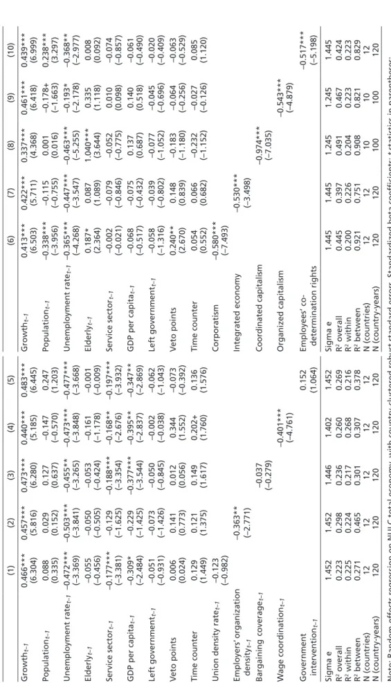
For the overall economy (Table 2), the results are as follows: growth shows a significant positive effect throughout all equations. According to the causal path discussed in Sec- tion 2, this is the anticipated result. In substantial terms, this result shows that, if there is a one-percent increase in GDP (as compared to the previous year), the expected NULC increase is between .3 and .4 percent (depending on the model).21 Furthermore, as we have argued, the regime-type variables impart independent negative effects on NULC increases. Seven out of ten measures show highly significant coefficients in the expected direction (p<.001); another two point in the expected direction but are not significant.
In five out of the seven cases with high significance – corporatism, integrated economy, coordinated capitalism, organized capitalism, and company-level codetermination – the regime effect outperforms the growth effect, which supports our claim that our understanding of the exchange rate distortions in the Eurozone must have two legs to stand on, an economic and a political science one.
Let us also consider why the remaining variables – bargaining coverage, union den- sity, and government intervention – have very low effects and no sufficient explana- tory power. Formal bargaining coverage and union density do not necessarily indicate coordination. Collective agreement coverage is below average in Germany, but these statistics hide a substantial number of firms without formal coverage that neverthe- less use such agreements as points of reference. Also, high degrees of coverage can go hand in hand with wage bargainers who compete along sectoral and ideological lines,
Ghali (1999); with regard to the Eurozone, see Collignon (2009: 430–431), Flassbeck/Lapavitsas (2013: 8–9), and Jones (2011: 293–294).
20 The correlations are r=.59 (NULC increases, overall economy), r=.63 (NULC increases in man- ufacturing), r=.72 (price inflation), and r=–.81 (current account surpluses).
21 Please note that the results show the standardized coefficients. This substantial interpretation comes from the unstandardized model solution, which is not shown but can be made available upon request.
as is the case in Spain. The same holds true for the share of union members among all employees. However, note the direction of the insignificant effect: strong nominal wage pressure tends to go together with weak trade unions, a remarkable fact with respect to the Troika’s union-busting strategies in Southern Europe (we will come back to this in the conclusion). In the case of our government-intervention variable, the effect is very close to zero, and even the sign points in the unexpected direction (i.e., intervention is associated with insignificantly higher NULC increases). Obviously, government inter- vention in wages does not necessarily suppress wage inflation but rather indicates the presence of a problem – and it is definitely no substitute for historically grown wage coordination among social partners.
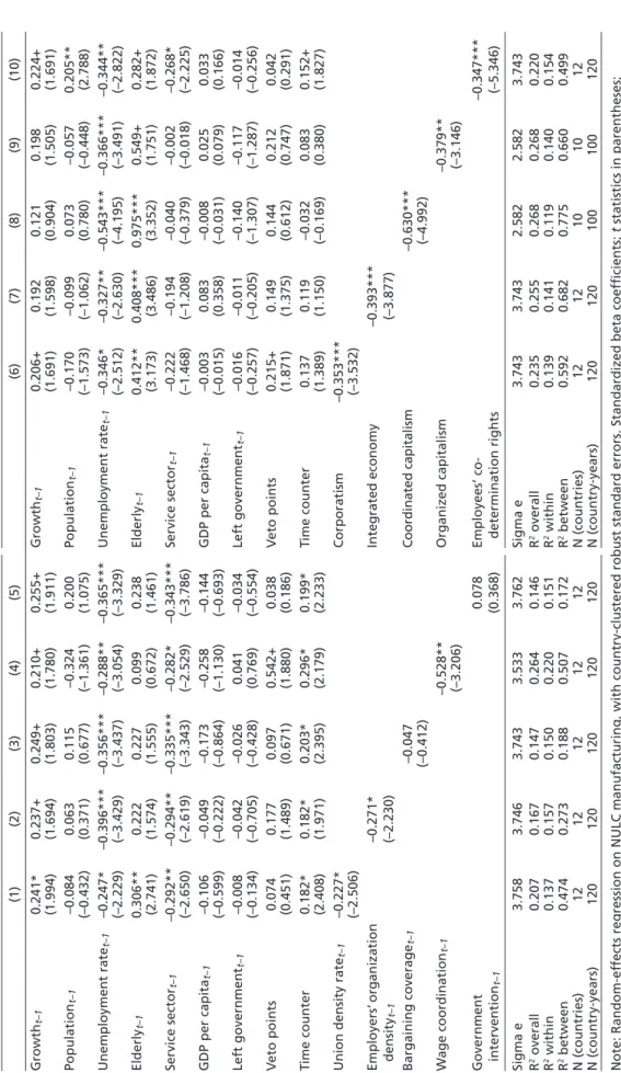
Table 3 reports the results for the manufacturing sector, which we treat as a proxy for the internationally exposed sector. Recall that the average wage increases were lower in this sector than in the overall economy, but the deviation from the mean was even larger here than in the overall economy (see Table 1). What explains this remarkable variance? Interestingly, the answer is not GDP growth. The growth variable shows only small effects across all models. Only in one out of ten models is growth significant at the 5-percent level. In all other models, growth has a rather small or insignificant effect (but its positive sign still points in the expected direction).
However, in eight out of ten cases, we find strong and highly significant regime-type effects. This holds true for union density, employers organization density, wage coordi- nation, corporatism, the integrated economy, coordinated capitalism, organized capital- ism, and company-level social partnership. Again, the bargaining-coverage coefficient points in the expected direction but lacks significance, and also again, the government- intervention effect is not only close to zero but also points in the wrong direction. We conclude that the industrial regime partly determines NULC inflation both in the over- all economy and in the exposed sector; while growth explains a significant part of the variance in NULC changes in the overall economy, this effect is absent or small in the exposed sector. In other words, whether or not the manufacturing sector could main- tain or even enhance its competitiveness during the first ten euro years was driven to a significant degree by the structure of the respective country’s industrial relations regime.
As for the control variables, the following results remain strong and robust across all models (both Tables 2 and 3): among the sociodemographic covariates, the unemploy- ment rate and service sector show negative effects on NULC increase. The higher a coun- try’s unemployment rate and the more developed its service sector – controlled for eco- nomic growth – the lower the increases in NULC are. The variable Elderly, the population over 65 as a percentage of the total population, shows positive effects in a few models, especially for the exposed sector. The political controls show no substantial effects but are important in ruling out possible differences due to political-constitutional structures.
Table 2Regression results for NULC total economy (1)(2)(3)(4)(5)(6)(7)(8)(9)(10) Growth t–10.466***0.457***0.473***0.440***0.483***Growth t–10.413***0.422***0.337***0.461***0.439*** (6.304)(5.816)(6.280)(5.185)(6.445)(6.503)(5.711)(4.368)(6.418)(6.999) Population t–10.0880.0290.127–0.1470.247Population t–1–0.338***–0.1150.001–0.178+0.238*** (0.335)(0.152)(0.637)(–0.570)(1.203)(–3.956)(–0.755)(0.016)(–1.663)(3.297) Unemployment rate t–1–0.472***–0.503***–0.455**–0.473***–0.477***Unemployment rate t–1–0.365***–0.447***–0.463***–0.193*–0.368** (–3.369)(–3.841)(–3.265)(–3.848)(–3.668)(–4.268)(–3.547)(–5.255)(–2.178)(–2.977) Elderly t–1–0.055–0.050–0.053–0.161–0.001Elderly t–10.187*0.0871.040***0.3350.008 (–0.456)(–0.505)(–0.424)(–1.178)(–0.009)(2.364)(1.089)(3.644)(1.118)(0.092) Service sector t–1–0.177***–0.129–0.188***–0.168**–0.197***Service sector t–1–0.002–0.079–0.0520.010–0.074 (–3.381)(–1.625)(–3.354)(–2.676)(–3.932)(–0.021)(–0.846)(–0.775)(0.098)(–0.857) GDP per capita t–1–0.309*–0.229–0.377***–0.395**–0.347**GDP per capita t–1–0.068–0.0750.1370.140–0.061 (–2.484)(–1.425)(–3.544)(–2.837)(–2.869)(–0.517)(–0.432)(0.687)(0.518)(–0.490) Left government t–1–0.051–0.073–0.050–0.002–0.062Left government t–1–0.058–0.039–0.077–0.045–0.020 (–0.931)(–1.426)(–0.845)(–0.038)(–1.043)(–1.316)(–0.802)(–1.052)(–0.696)(–0.409) Veto points0.0060.1410.0120.344–0.073Veto points0.240**0.148–0.183–0.064–0.063 (0.024)(0.773)(0.056)(1.552)(–0.392)(2.670)(0.839)(–1.180)(–0.256)(–0.529) Time counter0.1290.1210.1490.202+0.136Time counter0.0540.066–0.232–0.0270.085 (1.449)(1.375)(1.617)(1.760)(1.576)(0.552)(0.682)(–1.152)(–0.126)(1.120) Union density rate t–1–0.123Corporatism–0.580*** (–0.982)(–7.493) Employers’organization density t–1–0.363** (–2.771)Integrated economy–0.530*** (–3.498) Bargaining coverage t–1–0.037Coordinated capitalism–0.974*** (–0.279)(–7.035) Wage coordination t–1–0.401***Organized capitalism–0.543*** (–4.761)(–4.879) Government intervention t–10.152 (1.064)Employees’ co determination rights–0.517*** (–5.198) Sigma e1.4521.4521.4461.4021.452Sigma e1.4451.4451.2451.2451.445 R2 overall0.2230.2980.2360.2600.269R2 overall0.4450.3970.4910.4670.424 R2 within0.2250.2240.2170.2680.216R2 within0.2000.2260.2040.2230.223 R2 between0.2710.4650.3010.3070.378R2 between0.9210.7510.9080.8210.829 N (countries)1212121212N (countries)1212101012 N (countryyears)120120120120120N (countryyears)120120100100120 Note: Randomeffects regression on NULC total economy, with countryclustered robust standard errors. Standardized beta coefficients; t statistics in parentheses; + p < 0.1, * p < 0.05, ** p < 0.01, *** p < 0.001 (twosided tests).
Table 3Regression results for NULC manufacturing (1)(2)(3)(4)(5)(6)(7)(8)(9)(10) Growth t–10.241*0.237+0.249+0.210+0.255+Growth t–10.206+0.1920.1210.1980.224+ (1.994)(1.694)(1.803)(1.780)(1.911)(1.691)(1.598)(0.904)(1.505)(1.691) Population t–1–0.0840.0630.115–0.3240.200Population t–1–0.170–0.0990.073–0.0570.205** (–0.432)(0.371)(0.677)(–1.361)(1.075)(–1.573)(–1.062)(0.780)(–0.448)(2.788) Unemployment rate t–1–0.247*–0.396***–0.356***–0.288**–0.365***Unemployment rate t–1–0.346*–0.327**–0.543***–0.366***–0.344** (–2.229)(–3.429)(–3.437)(–3.054)(–3.329)(–2.512)(–2.630)(–4.195)(–3.491)(–2.822) Elderly t–10.306**0.2220.2270.0990.238Elderly t–10.412**0.408***0.975***0.549+0.282+ (2.741)(1.574)(1.555)(0.672)(1.461)(3.173)(3.486)(3.352)(1.751)(1.872) Service sector t–1–0.292**–0.294**–0.335***–0.282*–0.343***Service sector t–1–0.222–0.194–0.040–0.002–0.268* (–2.650)(–2.619)(–3.343)(–2.529)(–3.786)(–1.468)(–1.208)(–0.379)(–0.018)(–2.225) GDP per capita t–1–0.106–0.049–0.173–0.258–0.144GDP per capita t–1–0.0030.083–0.0080.0250.033 (–0.599)(–0.222)(–0.864)(–1.130)(–0.693)(–0.015)(0.358)(–0.031)(0.079)(0.166) Left government t–1–0.008–0.042–0.0260.041–0.034Left government t–1–0.016–0.011–0.140–0.117–0.014 (–0.134)(–0.705)(–0.428)(0.769)(–0.554)(–0.257)(–0.205)(–1.307)(–1.287)(–0.256) Veto points0.0740.1770.0970.542+0.038Veto points0.215+0.1490.1440.2120.042 (0.451)(1.489)(0.671)(1.880)(0.186)(1.871)(1.375)(0.612)(0.747)(0.291) Time counter0.182*0.182*0.203*0.296*0.199*Time counter0.1370.119–0.0320.0830.152+ (2.408)(1.971)(2.395)(2.179)(2.233)(1.389)(1.150)(–0.169)(0.380)(1.827) Union density rate t–1–0.227*Corporatism–0.353*** (–2.506)(–3.532) Employers’organization density t–1–0.271* (–2.230)Integrated economy–0.393*** (–3.877) Bargaining coverage t–1–0.047Coordinated capitalism–0.630*** (–0.412)(–4.992) Wage coordination t–1–0.528**Organized capitalism–0.379** (–3.206)(–3.146) Government intervention t–10.078 (0.368)Employees’ co determination rights–0.347*** (–5.346) Sigma e3.7583.7463.7433.5333.762Sigma e3.7433.7432.5822.5823.743 R2 overall0.2070.1670.1470.2640.146R2 overall0.2350.2550.2680.2680.220 R2 within0.1370.1570.1500.2200.151R2 within0.1390.1410.1190.1400.154 R2 between0.4740.2730.1880.5070.172R2 between0.5920.6820.7750.6600.499 N (countries)1212121212N (countries)1212101012 N (countryyears)120120120120120N (countryyears)120120100100120 Note: Randomeffects regression on NULC manufacturing, with countryclustered robust standard errors. Standardized beta coefficients; t statistics in parentheses; + p < 0.1, * p < 0.05, ** p < 0.01, *** p < 0.001 (twosided tests).