This research has been financed by ITARS (www.itars.net), European Union Seventh Frame-

L idar and M icrowave R adiometer S ynergy for H igh V ertical R esolution T hermodynamic P rofiling .

María Barrera Verdejo

ing.

This research has been financed by ITARS (www.itars.net), European Union Seventh Frame-

work Programme FP7: People, ITN Marie Sklodowska Curie Actions Programme under grant

agreement no 289923.

L idar and M icrowave R adiometer S ynergy for H igh V ertical R esolution T hermodynamic P rofiling .

I n a u g u r a l - D i s s e r t a t i o n

zur

Erlangung des Doktorgrades

der Mathematisch-Naturwissenschaftlichen Fakultät

der Universität zu Köln

vorgelegt von

María Barrera Verdejo

aus Granada, Spanien

Köln

2016

Prof. Dr. Susanne Crewell Universität zu Köln PD Dr. Ulrich Löhnert Universität zu Köln

Prof. Dr. Bjorn Stevens Max-Planck-Institute für Meteorologie

Tag der letzten mündlichen Prüfung: 27th of May 2016

A mi familia y a Jose. Ellos ya saben el resto.

Nothing in life is to be feared.

It is to be understood.

Now is the time to understand more, so that we may fear less.

Marie S. Curie

F oreword

Planet Earth is simply fascinating, exhibiting countless ways of life. As a result of evolution, they fit and function seamlessly, in equilibrium. Earth’s arrangement and complexity allow us to inhabit this place. Three large subsystems form this planet: its solid part (lithosphere), which is mainly covered by water (hydrosphere) and the gaseous component (atmosphere), which surrounds the two other. The three of them are strongly interrelated and their current configuration permit life on Earth.

For example, have you ever wondered what planet Earth would look like without atmo- sphere? For sure, it would be very different. And most probably, life as it is understood nowadays, would not be possible at all. The reason for that is simple: this most external layer is the blanket that tucks our planet. It creates a closed thermodynamic system that avoids icy nights and extremely hot days. In addition, thanks to the ozone layer, most of the ultraviolet radiation emitted by the Sun is absorbed. The atmosphere also acts as shield against meteorites. What else can we ask for? We owe a lot to our atmosphere.

More technically, the atmosphere is a thin shell around planet Earth that has a thickness greater than 100 km and a mass of ∼ 5.1 · 10 ¹⁸ kg. It might be surprising to learn that 75% of the atmospheric mass is concentrated in the lowest ∼ 11 km: the troposphere, which contains the 99%

of the total atmospheric water vapor. In addition, the strongest atmospheric interactions take place in layers closest to the ground, where land surface energy exchanges make the full story a complex adventure. A lot of things are continuously going on in there: it is the Times Square of the atmosphere!

For these reasons and more, the lower troposphere awakens special interest in human beings.

This interest is the basis for the current thesis, and probably the reason why we both are here:

you, reading these words, and I, writing them.

C ontents

Zusammenfassung xi

Abstract xiii

1 Introduction 1

1.1 Motivation . . . . 1

1.2 State of the art . . . . 3

1.3 Goals of the thesis . . . . 5

2 Instrumentation and data 7 2.1 Measurement campaigns . . . . 7

2.1.1 HD(CP) ² Observational Prototype Experiment: HOPE . . . . 7

2.1.2 Next-Generation Aircraft Remote sensing for Validation Studies: NARVAL 8 2.2 Microwave radiometer . . . 10

2.2.1 Radiative transfer . . . 11

2.2.2 Humidity and Temperature Profiler: HATPRO . . . 14

2.2.3 HALO Microwave Package: HAMP . . . 15

2.3 Lidar: Light Detection and Ranging . . . 16

2.3.1 Lidar theory . . . 16

2.3.2 The University of Basilicata Raman lidar system: BASIL . . . 20

2.3.3 WAter vapor Lidar Experiment in Space: WALES . . . 21

2.4 Auxiliary data . . . 22

2.4.1 Radiosondes and dropsondes . . . 22

2.4.2 Global Positioning System . . . 23

2.4.3 JOYRAD35 radar . . . 24

2.4.4 Ceilometer . . . 24

2.4.5 Cloudnet . . . 24

2.4.6 ERA-Interim reanalysis . . . 25

2.5 Summary . . . 25

3 Algorithm 27 3.1 Optimal Estimation theory . . . 27

3.2 LIME SOAP . . . 29

3.2.1 A priori information and atmospheric state . . . 30

3.2.2 Instrument data . . . 35

3.2.3 Forward models . . . 39

3.3 Summary . . . 41

4 Absolute humidity retrieval - ground based 43 4.1 Case study . . . 43

4.2 Statistical assessment . . . 46

4.2.1 IWV assessment using GPS . . . 47

4.2.2 Comparison with radiosondes . . . 48

4.2.3 Theoretical error . . . 50

4.2.4 Information content analysis . . . 56

4.3 Summary . . . 59

5 Temperature and relative humidity retrieval 61 5.1 Temperature . . . 61

5.1.1 Case study . . . 62

5.1.2 Statistical assessment . . . 64

5.2 Relative humidity . . . 66

5.3 Summary . . . 67

6 Profiling of the cloudy atmosphere 69 6.1 Cloud remote sensing . . . 69

6.2 Retrieval in cloudy scenario . . . 76

6.2.1 Thermodynamic profiles . . . 76

6.2.2 Liquid water path and integrated water vapor . . . 78

6.3 Summary . . . 79

7 Application to airborne data: HALO 81 7.1 The airborne perspective . . . 81

7.1.1 A priori . . . 82

7.1.2 MWR measurement bias . . . 84

C ontents

7.2 Absolute humidity retrieval . . . 85

7.2.1 Comparison to DS . . . 85

7.2.2 Information content . . . 86

7.3 Temperature retrieval . . . 87

7.3.1 Comparison to DS . . . 87

7.3.2 Information content . . . 88

7.4 Relative humidity retrieval . . . 88

7.5 Time series . . . 89

7.6 Summary . . . 93

8 Conclusions 95

Bibliography 99

Appendix 107

Erklärung 109

About the author 111

Acknowledgments 113

Z usammenfassung

Kontinuierliche Beobachtungen thermodynamischer Vertikalprofile der Atmosphäre spielen für

zahlreiche Anwendungen, wie etwa die Bestimmung der atmosphärischen Stabilität oder der

Wolkenbildung, eine wichtige Rolle. Heutzutage stehen zahlreiche bodengebundene Sensoren

zur Verfügung, um diese Vertikalprofile abzuleiten. Allerdings ist keines dieser Instrumente

momentan in der Lage, gleichzeitig sowohl eine hohe vertikale und zeitliche Auflösung über

den gesamten Höhenbereich zu gewährleisten, als auch bei allen Wetterbedingungen verläs-

sliche Messwerte zu liefern. Aus diesen Gründen wurde in der Atmosphärenwissenschaft im

letzten Jahrzehnt vermehrt der Fokus auf die Nutzung von Synergien verschiedener Instrumen-

te gelegt, um die Qualität und Nutzbarkeit bestehender Messungen zu verbessern. Die hier

vorgelegte Doktorarbeit stellt ein Verfahren vor, welches die Synergie von Mikrowellenradiome-

ter (MWR) und Lidar nutzt, um spezifische Einschränkungen der einzelnen Messverfahren zu

überwinden. Lidarmessungen sind in der Lage, Profile der Temperatur und des Wasserdampfs

mit hoher vertikaler Auflösung zu liefern. Jedoch sind die Messungen beschränkt bezüglich

der maximalen Messhöhe, bedingt durch die Problematik der Überlappungsfunktionen (OVF)

und Beeinträchtigungen durch Sonnenlicht und Wolken. Dem gegenüber erlauben MWR die

Ableitung von Temperatur- und Wasserdampfprofilen und Informationen über Wolken aus dem

gesamten Troposphärenbereich, allerdings mit geringer vertikaler Auflösung. Der in dieser Ar-

beit vorgestellte Retrieval-Algorithmus „Lidar and Microwave Synergetic Optimal Atmospheric

Profiler (LIME SOAP)” kombiniert die Beobachtungen dieser zwei Messgeräte basierend auf der

sogenannten „Optimal Estimation” Methode (OEM). Der wesentliche Vorteil dieser Methode

im Gegensatz zu anderen Ansätzen, wie etwa neuralen Netzen, Kalman-Filtern, usw., besteht

darin, dass die OEM eine Fehlerabschätzung des abgeleiteten atmosphärischen Produktes er-

laubt. In LIME SOAP werden Beobachtungen, d.h. MWR-Helligkeitstemperaturen und Lidar-

Wasserdampfmischungsverhältnisse und / oder Temperaturprofile, mit a priori-Informationen der

Atmosphäre kombiniert, wobei die Unsicherheiten in beiden Quellen berücksichtigt werden. Die

Methode wurde auf zwei unterschiedliche Datensätze angewendet, um vertikal hochaufgelöste Profile der absoluten Feuchte (AH), Temperatur (T), relativen Feuchte (RH) und Flüssigwasser- pfad (LWP) abzuleiten. Ein bodengebundener Datensatz wurde während einer zweimonatigen Messkampagne in Deutschland aufgenommen. Ein zusätzlicher Flugzeugdatensatz entstand während einer Kampagne über dem tropischen und subtropischen Atlantik. Für alle erzeugten Retrievals ergaben die Untersuchungen des theoretisch erwartbaren Fehlers und der Freiheits- grade des Signals, dass die Informationen der beiden Instrumente mit dieser Methode optimal kombiniert werden konnten. Des Weiteren konnte die Vertikalauflösung des abgeleiteten Pro- dukts durch die MWR-Lidar-Synergie im Vergleich zum Einzelinstrument verbessert werden.

In verschiedenen Experimenten wurden die Verbesserungen durch die Instrumentensynergie

im Vergleich zu den Resultaten der einzelnen Messgeräte analysiert. Die Resultate für einen

zweimonatigen, bodengebundenen Datensatz zeigen beispielsweise, dass der durchschnittliche

theoretische Fehler im absoluten Feuchteprofil bei der LIME SOAP-Methode um 60% (38%)

reduziert werden konnte in Bezug auf Resultate, welche ausschließlich MWR (Raman Lidar)

Daten nutzen. Der Fehler der Temperaturmessung konnte um 47.1% (24.6%) reduziert werden

im Vergleich zu den Methoden mit ausschließlich MWR (Raman Lidar), wobei die Profile nahe-

gelegenen Radiosondenaufstiege als Referenz herangezogen wurden. Bei der Ableitung der RH

wurden Korrelationen zwischen T und AH miteinbezogen, was zu Verbesserungen im abgelei-

teten RH Profil führte im Vergleich zum RH-Profil basierend auf einer unabhängigen Ableitung

von T und AH. Des Weiteren konnte gezeigt werden, dass das T Profil aus dem Raman Lidar

nicht unbedingt notwendig für die abgeleiteten T- und RH-Profile ist, sondern dass bereits das

T Profil aus den MWR-Messungen für die durchgeführten Fallstudien zu zufriedenstellenden

Ergebnissen führt. Bei der Messgeometrie mit Messflugzeugen wie etwa HALO, liegt der nicht

überlappende Messbereich des Lidars in der oberen Troposphäre, also in einem Bereich mit ge-

nerell geringem Wasserdampfgehalt. Daher erzielen die MWR Messungen in dieser Region ohne

Lidardaten einen geringeren positiven E ff ekt verglichen mit der bodengebundenen Messanord-

nung. Die Vorteile der Sensorkombination konnten in dieser Arbeit klar demonstriert werden,

wobei sich die größten Verbesserungen in Höhenbereichen ergaben, in denen Lidarmessungen

nicht verfügbar waren. In Bereichen, in denen beide Messgeräte Daten lieferten, dominierten die

Lidarmessungen die kombinierten abgeleiteten thermodynamischen Profile.

A bstract

Continuous monitoring of thermodynamic atmospheric profiles is important for many appli- cations, e.g. assessment of atmospheric stability and cloud formation. Nowadays there is a wide variety of ground-based sensors for atmospheric profiling. Unfortunately there is no single instrument able to provide a measurement with complete vertical coverage, high vertical and temporal resolution, and good performance under all weather conditions, simultaneously. For this reason, in the last decade instrument synergies have become a strong tool used by the scien- tific community to improve the quality and usage of the atmospheric observations. The current thesis presents the microwave radiometer (MWR) and lidar synergy, which aims to overcome the specific sensor limitations.

On the one hand, lidar measurements can provide water vapor or temperature measurements with a high vertical resolution albeit with limited vertical coverage, due to overlapping function (OVF) problems, sunlight contamination and the presence of clouds. On the other hand, MWRs receive water vapor, temperature and cloud information throughout the troposphere though their vertical resolution is poor. The retrieval algorithm combining these two instruments is called Lidar and Microwave Synergetic Optimal Atmospheric Profiler (LIME SOAP) and is based on an Optimal Estimation Method (OEM). The main advantage of this technique with respect to other retrieval algorithms, e.g. neural networks, Kalman filters, etc., is that an OEM allows for an uncertainty assessment of the retrieved atmospheric products.

LIME SOAP combines measurements, i.e. MWR brightness temperatures and lidar water vapor mixing ratio and/or temperature profiles, with a priori atmospheric information taking the uncertainty of both into account. The method is applied to two different scenarios, i.e. ground based measurements during a two months campaign in Germany, and airborne measurements over tropical and subtropical Atlantic Ocean, for retrieving high vertical resolution profiles of absolute humidity (AH), temperature (T), relative humidity (RH) and liquid water path (LWP).

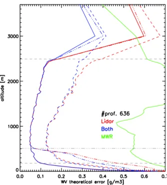
For all retrievals, the studies in terms of theoretical error and degrees of freedom per signal reveal

that the information of the two sensors is optimally combined. In addition, the vertical resolution of the products is improved when the MWR+lidar combination is performed with respect to the instruments working alone.

Different experiments are performed to analyze the improvements achieved via the synergy compared to the individual retrievals. Results show that, for example, when applying the LIME SOAP for ground-based AH profiling, on average the theoretically determined absolute humidity uncertainty is reduced by 60% (38%) with respect to the retrieval using only-MWR (only-Raman lidar) data, for two-months data analysis. For temperature, it is shown that the error is reduced by 47.1% (24.6%) with respect to the only-MWR (only-Raman lidar) profile, when using a collocated radiosonde as reference.

When retrieving RH, correlation between T and AH is included, which leads to improvements in the retrieved RH with respect to the case when T and AH are calculated independently. In addition it is shown that the Raman lidar T profile is not essential for the T and RH retrievals and using only the MWR temperature information provides products satisfactory for the specific case study. From the airborne perspective of HALO, the lidar non-overlap region is situated in the upper troposphere, where the amount of water vapor is reduced. Thus, the MWR improvement in the blind lidar region has less impact than in the ground based scenario.

The benefits of the sensor combination are demonstrated, being especially strong in regions

where lidar data is not available, whereas if both instruments are available, the lidar measure-

ments dominate the retrieval.

1

I ntroduction

Climate change is one of the largest challenges for mankind. Still, the changes to be expected in the distribution of temperature and precipitation strongly vary between different climate models.

How clouds and the formation/suppression of precipitation will develop is a long lasting question and a major reason for the differences between models. But which — if any — is giving the truth?

What role do environmental conditions like water vapor and temperature play?

In order to answer these questions, it is essential to better understand the atmospheric phe- nomena. Observations are essential for the understanding of atmospheric processes, since for a long time hardly any quantitative measurements of atmospheric parameters existed. Because in situ measurements are not possible everywhere, one must resort to remote sensing techniques, whose development has been fostered only in recent times by technological progress.

1.1 M otivation

Water vapor and temperature are essential variables required for the understanding of many atmospheric phenomena. According to Hoff and Hardesty (2012), temperature and moisture profiling in the lower troposphere are central to some of the most important research and opera- tional goals in atmospheric and Earth system studies, mesoscale numerical weather prediction, and monitoring of regional climate variability. Water vapor is not only the most important green- house gas, but also its radiative properties influence the planetary albedo, and hence Earth’s surface temperature, as well as the hydrological cycle and the thermodynamic structure of the troposphere (Stevens and Bony, 2013).

Already twenty years ago, Crook (1996) stated that variations in boundary layer temperature

and moisture within 1 ^◦ C and 1 g/kg respectively, can make the difference in prediction models

between no initiation and intense convection, which hints at the accuracy needed for the ob-

servations. More recent research (Hoff and Hardesty, 2012) summarizes the requirements for

measurements in order to be able to resolve short time scale processes, i.e. 30 meters in hori- zontal and vertical resolution, with a repeatability of 1 second and precision of 5% and 0.2 K for humidity and temperature respectively. These requirements present a challenge to tackle despite the fact that a wide variety of ground based, airborne and satellite remote sensing instruments that sense atmospheric parameters exist.

Remote sensing instruments measure passively or actively different atmospheric features in several spectral domains (infrared, visible, microwave, etc.), each providing di ff erent and com- plementary information about the atmospheric state. Nevertheless, even if there is a wide variety of atmospheric sensors, there is none which can provide all of the following requirements simul- taneously: complete vertical coverage, high vertical and temporal resolution of the atmospheric profiles and satisfactory performance under all weather conditions. Specifically, processes on short time scales such as convection, cloud formation or boundary layer turbulence cannot be resolved completely by any single instrument alone. In order to overcome this limitation, the scientific community started in the last decade to perform instrument synergies, merging data from different sensors.

In the present thesis, the synergy between two different remote sensing instruments is pre- sented: lidar and Microwave Radiometer (MWR). They are used to retrieve temperature and humidity atmospheric profiles. Both instruments present several advantages and drawbacks.

Nevertheless, it is possible to overcome some of the disadvantages in the single devices and enhance their benefits by combining them in an optimal and new retrieval algorithm: the Lidar and Microwave Synergetic Optimal Atmospheric Profiler (LIME SOAP).

On the one hand, lidar systems provide highly vertically resolved measurements of atmo-

spheric humidity profiles. For this reason, lidars have become a strong tool for active observations

in the last years and new retrieval algorithms optimally exploiting the information content are

developed (Sica and Haefele, 2015; Povey et al., 2014). However, the lidar technique presents im-

portant weaknesses, which might hinder its operational application. For example, lidars cannot

provide information above and within optically thick clouds, as the radiation emitted by the lidar

quickly extinguishes once the laser beam reaches a cloud. Moreover, day time measurements

can be affected by background solar radiation, which strongly reduces the vertical range of the

measurements. The continuous and effective detection of lidar signals, which are typically weak,

requires robust and stable receiving systems. Daytime operation is not possible in all cases and

requires the use of powerful lasers whose continuous operation is technically demanding. Addi-

tionally, most of the lidars need to be calibrated. This calibration is usually performed based on

the use of radiosounding data, which presents some caveats. First, the balloon might measure

a different air volume due to its drift. Second, it implies both a high human and instrument

cost. The calibration of the lidar is a key point that still represents a scientific challenge (Foth

et al., 2015). In addition, the information of the layers closest to the instrument typically cannot

be used, due to the presence of a blind region associated with the overlap function (OVF) of the

1.2 S tate of the art system.

On the other hand, the MWR allows continuous passive data acquisition and it is a robust operational instrument (Rose et al., 2005), measuring unattended in a 24/7 mode. In contrast to lidars, the instrument offers a much more limited vertical resolution of the retrieved atmospheric profiles, especially in higher layers of the atmosphere (i.e. 1 km away from the instrument) (Löhnert et al., 2007). Nevertheless, MWR performs best for measurements close to the instru- ment, where there are no lidar data. MWR also provides accurate integrated quantities such as Integrated Water Vapor (IWV) or Liquid Water Path (LWP) . The calibration of this instrument is performed with internal references with known temperature (hot load-cold load) or by observ- ing the atmosphere under different elevation angles (i.e. sky tipping) (Maschwitz et al., 2013).

Another advantage of the MWR is the capability of measuring in almost all weather conditions (also cloudy cases) except for rainy scenarios, where the received signal must be discarded in most of the cases.

1.2 S tate of the art

Several ground-based synergies have been performed previously. For example, Stankov (1998) combined ground- and space- base remote sensing measurements, i.e. passive radiometric, radar, and in situ observations, to estimate the temperature and humidity profiles. Her retrieval has two stages, the first starting with a simple linear statistical inversion using ground-based measure- ments, whose result serves as a priori information for the second stage. The latter is a traditional physical one step algorithm to iteratively adapt brightness temperatures to atmospheric pro- files. The author uses space-based radiance measurements from polar-orbiting satellites. When brightness temperature difference is below the instrument noise, convergence is achieved. The presented results were a real advance at that time: the retrieved temperature profiles present a bias of -0.27 ^◦ C and a standard deviation of 1.56 ^◦ C.

Humidity profiles have been also retrieved by Bianco et al. (2005), combining microwave

radiometry and wind profiler radar measurements. Their combination of passive and active

sensors relies on the relationship between the gradients of specific humidity, potential refractivity

and potential temperature in the atmosphere (Stankov et al., 2003). This technique has the

advantage that it is independent from in situ measurements, relying only on remote sensing

information. Nevertheless, it is limited to work well only during convective periods, when

turbulence is well developed. The authors present also several unsatisfactory cases in which the

combined technique did not have good performance. For the derivation of humidity profiles

from the remote sensing observations, they use an analytical method, but discuss the possibility

of using a statistical method similar to the one implemented by Stankov (1998), which might be

more robust. In addition, they use the integrated water vapor content by the MWR as constraint

for their retrievals.

The two latter retrieval techniques present some weaknesses: first, the retrieved atmospheric profile is not optimally calculated and second, the retrieval methods do not allow a posteriori uncertainty assessment of the result.

A synergetic optimal method, based also on the OEM, was performed by Löhnert et al.

(2004). The authors describe the Integrated Profiling Technique, in which they retrieve physically consistent profiles of temperature, humidity, and cloud liquid water content. They achieve it by combining ground-based multichannel microwave radiometer, cloud radar, lidar-ceilometer and ground-level measurements of standard meteorological properties. Nevertheless, in this study the vertical resolution of the retrieved humidity profiles is restricted to the MWR information content.

Not only from the ground based perspective, instrument synergies are also performed for airborne and satellite applications. For example, Delanoe and Hogan (2008), where the authors combine ground-based and spaceborne radar, lidar and infrared radiometer. Their method is also based on an OEM for retrieving profiles of extinction coe ffi cient, ice water content and effective radius in ice clouds. The algorithm uses the radar and lidar data together to find the combination of microphysical variables that best forward models the observations. They test it on synthetic profiles generated from aircraft microphysical observations and on real ground-based data. Unfortunately, the instruments they use do not provide any information on the humidity and temperature profiles, though the authors suggest in their conclusions that the inclusion of more observations could be incorporated into their scheme for such aim, which would allow the full cloud profile to be retrieved.

A method to combine Raman lidar (RL) and MWR was also proposed by Han et al. (1997), where the authors developed a two-stage algorithm to derive water vapor atmospheric profiles.

In the first stage, a Kalman filtering algorithm was applied using surface in situ and RL measure- ments. In the second stage, a statistical inversion technique was applied to combine the Kalman retrieval with the integrated water vapor of a two-channel MWR and climatological data. Their method showed that the synergy of these two sensors compensates for the individual sensor’s drawbacks. A continuation of this work was carried out by Schneebeli (2009). The author still followed the Kalman filter two-stage configuration, substituting the second step for an inversion based on an OEM. The observation vector in the OEM consists of the MWR brightness tempera- tures, and the lidar profile resulting from the Kalman filter is introduced as a priori information.

The method is applied to synthetic measurements and only one real measurements case study.

In both Han et al. (1997) and Schneebeli (2009), only water vapor profiles were retrieved.

Most recently, Navas-Guzmán et al. (2014) presented the water vapor and relative humidity profiles from lidar and microwave radiometry. The authors use an iterative method to calibrate the water vapor mixing ratio profiles retrieved from Raman lidar measurements with the MWR.

In addition they present a method to combine these water vapor Raman lidar profiles with

temperature profiles retrieved with the MWR. Their results are presented for 1 year data in

1.3 G oals of the thesis Granada, though their lidar only measures during night-time. However, their method does not combine the MWR and lidar measurements in an optimal way and does not provide an a posteriori uncertainty assessment.

1.3 G oals of the thesis

In this thesis a new flexible method to combine lidar and MWR measurements is developed for the retrieval of thermodynamic profiles: LIME SOAP. The algorithm is a new approach based on an Optimal Estimation Method (OEM), an iterative optimal and physically consistent method which provides the most probable atmospheric state. One of the main advantages of this method with respect to other retrieval techniques is that OEM allows for the retrieval uncertainty assessment and a posteriori evaluation of the retrieval information content.

First, LIME SOAP is applied to the ground-based perspective for humidity and tempera- ture retrievals. For that, the data collected during HOPE (HD(CP) ² Observational Prototype Experiment) is used, where a multitude of ground-based remote sensing instruments for the in- vestigation of boundary layer and cloud processes were operated (Steinke et al., 2014a; Behrendt et al., 2015; Foth et al., 2015). Second, LIME SOAP is applied to the airborne perspective of HALO (High Altitude and Long range research Aircraft) (Mech et al., 2014), which flew during the NARVAL (Next-Generation Aircraft Remote sensing for Validation Studies) campaign.

The main goal of this thesis is to quantify the value of the MWR and RL synergy for different viewing geometries and atmospheric conditions. For said purpose, in this work the details of how to perform an optimal MWR and RL synergy are explained. After the overview provided by the introduction, chapter 2 gives a general description of the field campaigns and the instruments used in this thesis. The MWR working principle and the radiative transfer equation are explained (section 2.2.1) together with the characteristics of the HATPRO (Humidity and Temperature Profiler, section 2.2.2) and HAMP (HALO Microwave Package, section 2.2.3) MWRs, operated during HOPE and NARVAL campaigns respectively. Two types of lidar are used and presented in this thesis: a Raman lidar, i.e. BASIL (section 2.3.2), and a Di ff erential Absorption lidar (DIAL), i.e. WALES (section 2.3.3). Section 2.4 explains the auxiliary data sources, e.g. reanalysis model data or radiosondes, which serve for retrieval evaluation or a priori information calculation in further chapters.

Chapter 3 provides a description of the synergetic algorithm. It first starts presenting the

general theory of an OEM, describing what are its main parts: a priori information, instrument

measurements, forward models and the retrieval information content assessment, i.e. averaging

kernels, theoretical error and degrees of freedom. The application of the OEM to the lidar and

MWR synergy for thermodynamic profiling is LIME SOAP. Section 3.2 describes the details on

how LIME SOAP components are modified, depending on the application, i.e. the retrieval

of different atmospheric variables, atmospheric scenarios or instrument geometry. Questions

related to the definition of a priori information or a forward model for each specific LIME SOAP application, are addressed in this part.

The application of LIME SOAP to the absolute humidity (AH) retrievals under clear sky conditions from the ground based perspective are presented in chapter 4. In order to demonstrate the MWR+lidar synergy, retrievals comparing the single instrument performance (i.e. LIME SOAP using only-RL data or using only-MWR data) to the combination of both (i.e. LIME SOAP using MWR + RL information) are presented. A case study profile first illustrates the synergy benefit in section 4.1. After that, section 4.2 presents the statistical assessment for the results of applying LIME SOAP to the complete HOPE period.

Because the two instruments have the capability of providing temperature (T) information, LIME SOAP is also applied to the T retrieval. That leads to the possibility of retrieving relative humidity (RH) information, which becomes especially valuable in the vicinity of clouds to study cloud formation. The T retrieval is described in chapter 5, together with the RH calculation (section 5.2). Comparisons to RS highlight the synergy benefits for T retrievals in section 5.1.1, followed by statistical assessment presented for a set of ∼ 150 retrieved profiles (section 5.1.2).

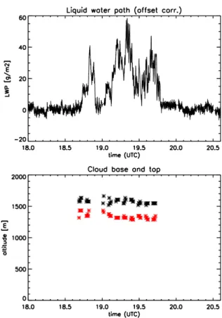
In addition, by including some information on cloud geometry, LIME SOAP can be extended to cloudy conditions, where the strongest synergy benefit is expected. The evaluation of the method applied to a simple cloudy scenario is described in chapter 6, where the MWR+RL signal turns essential to retrieve complete vertical T, AH and RH profiles. Results for a time series of these thermodynamic profiles are discussed in section 6.2.1. To provide information on the amount of water in the cloud, the liquid water path (LWP) is retrieved, together with integrated water vapor (IWV) calculations (section 6.2.2).

Completed the full ground based scenario, the synergy applied to the airborne perspective of HALO is exploited. The results of this application are discussed in chapter 7, where comparisons with auxiliary measurements and theoretical a posteriori studies show the synergy benefits.

Finally chapter 8 presents an overview of the thesis, highlighting the main results and opening

new ideas for further studies.

2

I nstrumentation and data

Two major field campaigns offer the opportunity to apply and test LIME SOAP using lidar and microwave radiometer (MWR) data. Firstly HOPE, deployed in Germany during spring 2013. Second, the NARVAL-South experiment, carried out flying through the tropical regions in December 2013. The two field experiments provide both lidar and MWR measurements, as well as auxiliary data for evaluation.

Firstly, this chapter will present these two field experiments (section 2.1). Second, the in- struments used in this thesis, focusing on the MWR (section 2.2) and lidar systems (section 2.3), whose working principle will be described in more detail, and completed with auxiliary data (section 2.4).

2.1 M easurement campaigns

2.1.1 HD(CP) ² O bservational P rototype E xperiment : HOPE

HOPE was a field campaign in Nordrhein-Westfalen, Germany, held from April to June 2013, as part of the HD(CP)2 project ¹ . The main goal of the campaign was to provide a complete high resolution picture of the clouds’ lifetime and evolution. During the measurement period, three supersites operated, distributed in the surroundings of Forschungszentrum Jülich (50.905N, 6.411944E), see figure 2.1. The supersites were situated at ∼ 4 km distance from each other. Each of them was composed of numerous remote sensing instruments, coordinated with di ff erent scanning strategies that allow the 3D study of clouds. A total of five Humidity and Temperature Profiler (HATPRO) radiometers and 3 lidar systems were operated, among other instruments.

1

HD(CP)2 (High Definition Clouds and Precipitation for Climate Prediction) is a major German-wide research ini- tiative to improve the understanding of cloud and precipitation processes and their implication for climate prediction.

For more information: http://hdcp2.zmaw.de ).

At the permanent supersite JOYCE (Jülich ObservatorY for Cloud Evolution) (Löhnert et al., 2014), measurements by the University of Basilicata Raman Lidar system (BASIL) and a HATPRO MWR were carried out. Auxiliary data from other instruments is available, such as ceilometers, cloud radar, micro-rain radar, total-sky imager, etc. Furthermore, more than 200 radiosondes (RS) were launched only ∼ 4 km away from JOYCE, at the KITCube supersite. The radiosondes were launched at least twice a day: at 11 and 23 UTC, and additionally launched during intensive observation periods.

Section 2.2.2 will describe the HATPRO radiometer in detail. In section 2.3.2, the Raman lidar (RL) BASIL will be presented. The additional data used for validation of the algorithm is described in section 2.4.

( a ) ( b )

F igure 2.1: (A) The JOYCE observatory at Jülich, Germany. (B) The three supersites operating during HOPE. A: JOYCE, B: KITCube & UHOH and C: LACROS. The red, yellow and greeen rings represent the 1 km, 2 km and 5 km distance around JOYCE, respectively. Source: Google maps.

2.1.2 N ext -G eneration A ircraft R emote sensing for V alidation S tudies : NARVAL The NARVAL campaign is an airborne mission, which aims for a better understanding of preva- lence and structure of clouds and precipitation from shallow convection (Klepp et al., 2014). The research airplane HALO ² (High Altitude and Long range research aircraft) (see figure 2.2) was equipped with a full array of state of the art remote sensing instruments (lidar, radiometers, radar, optical spectrometers), in situ sensors and additional instrumentation, e.g. dropsondes. The first mission is divided in two experiments with a total of 15 research flights: NARVAL-South, with

2

http://www.halo.dlr.de/

2.1 M easurement campaigns

( a )

( b )

F igure 2.2: (A) Open HALO bellypod, showing from left to right: the MWR (passive HAMP) in red, the lidar (WALES) in green and the radar (active HAMP) in yellow. (B) closed bellypod for flight operation. Source: Friedhelm Jansen, Max Planck Institute for Meteorology Hamburg.

focus on the subtropical region east of Barbados, in December 2013; and NARVAL-North, in the vicinity of Iceland in January 2014. The first is intended to study the trade wind regions;

the second focuses on postfrontal convective clouds and precipitation. In this study, the data collected during NARVAL-South has been used.

In total 8 research flights were carried out during NARVAL-South, between Oberpfaffenhofen

F igure 2.3: The NARVAL South mission flight pattern of the eight research flights over the North Atlantic tradewind region between Europe and Barbados. The squares represent the launched dropsondes and the red cross, the location of Barbados. Two dropsondes are highlighted, which will be used in further chapters. Source: S. Schnitt, personal communication.

(Germany) and the airport of Barbados, with 65-70 flight hours. Figure 2.3 gives an overview of the flights during the experiment. The goal of NARVAL-South was to fly over the northeast Atlantic trades to measure their evolution, compiling remote sensing measurements. Several flight legs were dedicated to satellite underflight for Cloudsat (Stephens et al., 2002) validation.

Additionally, 75 dropsondes were launched. More information on the campaign is found in Klepp et al. (2014). In this thesis, the radiometer HAMP (explained in section 2.2.3), the lidar WALES (section 2.3.3) and the dropsondes (section 2.4.1) will be used.

2.2 M icrowave radiometer

The microwave radiometer is a passive instrument, which measures thermal radiation emitted by the atmosphere in the microwave spectrum from 20-200 GHz (15-1.5 mm). Despite the fact that a MWR is a robust instrument that can measure in almost all weather scenarios, it presents a major drawback with respect to active instruments for profiling: its low vertical resolution, i.e.

only 2 pieces of information per profile for water vapor (Löhnert et al., 2007).

The radiatively significant atmospheric components in the microwave regime are gas molecules

and water, in the form of cloud droplets, precipitation or ice crystals. The radiation field is de-

termined by emission and extinction processes while propagating through the atmosphere. The

2.2 M icrowave radiometer extinction processes include absorption and scattering (radiation is redirected out of the prop- agation direction). The radiative transfer equation (RTE) describes the behavior of radiation propagating through the atmosphere. Based on the RTE, and measuring the radiation received by the MWR, one can analyze the atmospheric state. The RTE theory will be explained in this section, followed by the details of the two different MWR used in the next chapters.

2.2.1 R adiative transfer

The interactions among microwave radiation and atmospheric constituents are described with the RTE, whose theory is well described in the textbooks by Liou (1980) and Petty (2006) and will be explained shortly in the following.

Thermal emission is transmitted through the atmosphere, suffering extinction. The total atmospheric extinction is quantified by the extinction coefficient β e (in m ^{− 1} ), which accounts for the effects of atmospheric absorption (β a ) and scattering (β s ). The extinction coefficient has a frequency dependence in the microwave regime as depicted in figure 2.4. The peaks in the figure correspond to the absorption lines of the water vapor (around 22.235 and 183 GHz) and the oxygen absorption complex (around 60 and 118 GHz).

Because the scattering efficiency depends on the ratio of wavelength to particle size, the atmosphere can be approximated as a non-scattering medium for frequencies smaller than 100 GHz. The only exception occurs in the presence of large precipitation particles (Janssen, 1993).

By neglecting scattering, the radiation scenario is simplified to one dimension.

Consider the propagation of monochromatic radiation, with frequency ν, through an infinites- imal layer of air, whose thickness is dR. Its intensity of radiation I _ν (in _m

^W _s

sr ), which for the sake of simplicity will be referred as I in the following, will be reduced by absorption:

dI _abs = − β a · I · dR (2.1)

According to Kirchhoff’s Law, the absorption of any medium in local thermodynamic equi- librium is equal to the emissivity of the same matter. So one can expect the layer of air to emit radiation dI _emi . Thus, a net change in the radiation intensity through the infinitesimal layer of air can be then written as:

dI = dI _abs + dI _emi = − β a · I · dR + β a · B(T) · dR (2.2) or

dI = − β a · (B(T) − I) · dR (2.3)

which is the most general monochromatic form for the RTE, for a non-scattering medium.

This equation describes the change in radiation intensity at a frequency ν, while traversing an

absorptive medium, and is known as the Schwarzschild’s Equation (Petty, 2006). In equation

F igure 2.4: Extinction coefficient in the microwave spectrum at 850 hPa. The dashed line shows the water vapor contribution, the dotted line the oxygen contribution, and the dotted-dashed line the theoretical cloud liquid contribution of a cloud with 0.2gm

LWC, using the US-standard atmosphere. The solid line is the sum of all contributions. (Löhnert et al., 2004)

2.3, B(T) denotes the Planck function, which represents the thermal emission of a blackbody (emissivity = 1) at temperature T:

I = · B(T) ≈ B(T) = 2hν ³ c ²

1 e

− 1

(2.4)

where h is the Planck constant (h = 6.626 · 10 ^{− 34 m}

_s ^kg ), c is the speed of light in vacuum (c ≈ 3 · 10 ⁸ m/s) and k _b is the Boltzmann constant (k _b = 1.3810 ^{− 23 m} _sK

^kg ). Equation 2.4 relates the physical temperature to the intensity of radiation of an object , as a function of the radiation frequency. Because in the microwave regime the Rayleigh-Jeans approximation is valid ( _k ^hν

b

T 1),

one can approximate eq. 2.4 as follows:

B(T) = 2hk _b ν ² T

c ² (2.5)

which reveals a linear relation between the physical temperature and the blackbody radiation.

Therefore, the radiation intensity I is often scaled to an equivalent blackbody temperature, or brightness temperature T _B :

T _B ≡ B ^{− 1} (I) (2.6)

2.2 M icrowave radiometer where B ^{− 1} is the inverse of the Planck’s function solved for T assuming that the observed medium is a black body. This is the definition of the Planck equivalent brightness temperature, which in the Rayleigh-Jeans limit is equal to:

T _B = λ ²

2k _b I (2.7)

In practice, there are deviations between both, however the radiative transfer code used here considers the exact Planck solution. Thus, for a ground-based instrument receiving down- welling thermal radiation T _B

, using eq. 2.7 in 2.3 and integrating from ground to space, one can write the RTE as:

T _B

= T _B

e ^{− τ} + Z ^∞

0

β a (R)T(R)e ^{− τ(R)} dR (2.8)

which is the RTE for measurements taken from the ground-based perspective, under the assumption of plane-parallel atmosphere. T B

is the cosmic background radiation ( ∼ 2.73K (Janssen, 1993)), T(R) is the physical temperature. The term e ^{− τ} is the transmission term T _trans (R), and τ is the optical depth defined as:

τ(R) = Z R

0

β a (R ⁰ )dR ⁰ (2.9)

When the instrument is airborne based, the perspective and so the RTE changes. In addition to the upwelling radiation from the Earth surface and atmospheric components, also downwelling atmospheric radiation reflected by the surface needs to be considered. The MWR on HALO flies over the ocean, which has typically an emissivity of ≈ 0.5. depends on the frequency, the sea surface temperature (SST) and the surface wind. Combining all the radiation terms, the total brightness temperature at the altitude h at which an aircraft flies, is calculated by:

T B

(h) = T B

(h) + T B

(τ = τ 1 ) · e ^{− τ}

· (1 − ) (2.10)

with T B

(h) representing the thermal radiation emitted by the sea surface and the atmospheric layers, attenuated up to the aircraft:

T _B

(h) = · SST · e ^{− τ}

+ Z 0

h

β a (R)T(R)e ^{− τ (R)} dR (2.11) where τ 1 and τ 2 correspond to the optical depths in the path from infinite to the surface and from h to the surface, respectively. An example of the τ frequency dependence will be illustrated in figures 2.5 and 2.6 for the MWRs used in this thesis.

The form of the RTE in equation 2.8 will be used in chapters 4 to 6, for the ground-based

perspective. The RTE in equation 2.10 will be used in chapter 7, for the HALO scenario. In

the following, the MWR instruments used in the two different scenarios (ground- and airborne-

based) are presented.

2.2.2 H umidity and T emperature P rofiler : HATPRO

The microwave radiometer profiler HATPRO (Rose et al., 2005) was manufactured by Radiometer Physics GmbH, Germany (RPG) . It is a network-suitable microwave radiometer that allows to accurately retrieve at high temporal resolution (1 s) Liquid Water Path (LWP) and Integrated Water Vapor (IWV), with accuracies of 20 g/m ² and 0.5-1 kg/m ² , respectively (Löhnert and Crewell, 2003). It measures radiation in the atmosphere in two frequency bands in the K- and V-band. The seven channels of the K band contain information about the vertical profile of humidity through the pressure broadening of the optically thin 22.235-GHz H ₂ O line and contain also information for determining liquid water path. The seven channels of V-band, in the O ₂ complex (60 GHz), contain information on the vertical profile of temperature resulting from the homogeneous mixing of O ₂ throughout the atmosphere (Löhnert et al., 2009). The weighting functions for the K- and V-bands are presented in figure 2.5, showing the altitude sensitivity of all the 14 HATPRO channels. The instrument typically measures pointing zenith, but has also the capability of scanning. The inclusion of the angular information of the TB increases the vertical information content of the temperature retrieval, specially in the boundary layer (Crewell and Löhnert, 2007).

The voltages measured by the instrument need to be calibrated to an equivalent brightness temperature. An absolute calibration is performed taking a cold and a hot load as references, which are assumed to be ideal black bodies. The cold body is a liquid-nitrogen-cooled load that is attached externally to the radiometer box during calibration, which can be considered as a black body at the LN 2 boiling temperature of approximately 77 K. This standard, together with an internal ambient black body load (at ∼ 300 K), is used for the absolute calibration. The TBs absolute uncertainty is ± 0.5 K at the liquid nitrogen boiling temperature at all frequency channels, and increases towards colder T almost linearly (Küchler et al., 2016). In addition, a calibration by tip-curve observations is performed, whereby the instrument collects observations for the optically thin K-band channels at different elevation angles (Han and Westwater, 2000).

The reliability of sky tipping calibrations will strongly depend on how good the assumption of a horizontally stratified atmosphere is (Turner et al., 2007). Further details on the calibration procedures of the instrument can be found in Maschwitz et al. (2013) and Küchler et al. (2016).

The receiver antenna beam widths can be considered infinitively small (pencil beam approx-

imation), as discussed in Löhnert and Maier (2012). The radiometer radome is protected from

rain, snow and hail: a blower system is installed to dry it and prevent the formation of dew or

any possible condensation. The instrument receiver needs to be thermally stabilized with high

accuracy ( ± 0.1 K) for stable operation within the range of expected environmental conditions

(from -30 to +45 ^o K).

2.2 M icrowave radiometer

F igure 2.5: HATPRO clear sky weighting functions (zenith upward looking). Shown are the water vapor (left) and the temperature (right) weighting functions. The US 1976 Standard Atmosphere over a black surface was assumed for the calculations. Source: personal communication with M. Mech.

2.2.3 HALO M icrowave P ackage : HAMP

HAMP, the HAlo Microwave Package (Mech et al., 2014), is composed by two nadir-looking modules on board of HALO: first, the active component, which is a cloud radar at 36 GHz;

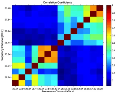
second, the passive microwave radiometers with 26 frequencies at different bands between 22.24 GHz and 183.31 GHz. In this thesis, only the passive microwave radiometer module is used and will be referred in the following as HAMP.

The HAMP MWR was custom manufactured for HALO by RPG and is mounted in the HALO

bellypod. It is composed of three modules. The first has receivers for the K- and V-band, similar to

HATPRO, where measurements in 14 different channels are taken. The second module measures

in a window channel at 90 GHz (W-band) and four channels in the 118.75 GHz ( ± 1.4 to ± 8.5

GHz) F-band, on the wing of an O ₂ absorption line. The last module measures radiation in the

183.31 GHz H ₂ O band ( ± 0.6 to ± 12.5 GHz), i.e. the G-band. All the three modules are thermally stabilized, with an accuracy < 0.05 K over the operation regime (from -70 to +35 ^o K).

The channels in the K-band and G-band are used for the retrieval of water vapor profiles and its integrated value (IWV). The channels in the V-band are used for T profiling, together with the four frequency channels in the F-band. The altitude sensitivity of the HAMP channels is shown in figure 2.6, which presents their clear sky weighting functions, calculated for the US 1976 Standard Atmosphere and assuming a ceiling height of 13 km. The figure nicely shows how the two innermost V-band channels present a high sensitivity to the temperature close to the aircraft. The outer channels of the G-band are less affected by water vapor and can be assumed to be window channels (Mech et al., 2014).

A liquid nitrogen calibration of the instrument was performed before every take off and after every landing. In addition, there is an in-flight calibration with two reference targets. One is at ambient temperature, corresponding to the stabilized temperature of the receiver box, and the second is generated by an internal noise diode producing a Gaussian distributed white noise signal. The beam width measured at full width at half maximum varies depending on the wavelength from 5.0 ^o in the K and V bands, to 2.7 ^o in the 183-module. This leads to a resolution at ground between 1.4 and 0.9 km in the along-flight direction and between 1.1 and 0.6 km in the across-flight direction (considering 13 km flying altitude and 1 s integration time).

2.3 L idar : L ight D etection and R anging

Lidar (Light Detection and Ranging) is a principle for active remote sensing measurements. A general lidar system transmits a narrow laser beam into the atmosphere and receives the scattered light back to the instrument. It can work in the ultraviolet, visible and near-infrared regimes, depending on the application. Due to historical reasons, wavelengths are preferred in the lidar community, while frequency is used in the MWR community.

Different types of lidar exist: Differential absorption lidar (DIAL) , Doppler lidar, Raman lidar, etc. according to the physical mechanism that is exploited. Below, the basic principle of a lidar system, together with the description of a Raman lidar and a DIAL is presented. In addition, the RL BASIL (section 2.3.2) and the DIAL WALES on HALO (section 2.3.3) are described. In this study, both instruments were used to measure atmospheric water vapor and only the RL measures atmospheric temperature as well.

2.3.1 L idar theory

The basic configuration of a lidar system consists of a transmitter and a receiver. The first

emits light pulses to the atmosphere, generated by a laser. The second collects the radiation

backscattered from the atmosphere by a telescope. This is followed by an ensemble of filters,

2.3 L idar : L ight D etection and R anging

F igure 2.6: HAMP clear air weighting functions (nadir downward looking). Shown are the water vapor (two leftmost) and the temperature (two rightmost) weighting functions for a HALO ceiling height of about 13 km. The US 1976 Standard Atmosphere over a black surface was assumed for the calculations. The figure is taken from Mech et al. (2014).

which select the part of the signal under interest. The selected optical signal arrives at a detector, where it is converted to an electrical signal.

The most general form to express the power P received on a lidar system from the distance R is (Weitkamp, 2005):

P(R) = K · G(R) · β(R) _π · T _trans (R) (2.12)

where K is a factor summarizing the system performance and G(R) is the range-dependent measurement geometry function (i.e. the overlapping function). These two terms depend only on the lidar system configuration. The terms β _π (R) and T _trans (R) are the backscatter coefficient and the transmission term at distance R, respectively.

The backscatter coefficient (in m ^{− 1} sr ^{− 1} ) describes how much radiation is scattered towards the instrument (i.e. 180 ^◦ scattering) and is frequency dependent. It is proportional to the number of scatterers in the atmosphere and to the backscattering cross section, i.e. probability of scattering in the direction of study. In the atmosphere, the emitted laser light is scattered by molecules (i.e.

nitrogen and oxygen) and by particles (aerosols, water droplets, etc.).

The transmission term T trans (R) represents the fraction of light that arrives at the receiver after propagating from the laser to the backscattering volume and back. T _trans (R) depends on the extinction coefficient α(R, λ) ³ , which accounts for the total transmission losses. The extinction co- efficient includes the contributions of scattering and absorption of light by atmospheric molecules and particles. The parameters β π (R) and T _trans (R) are the ones providing the information on the atmospheric state, since they depend on the atmospheric components.

Scattering can take place in di ff erent ways: elastically or inelastically. In contrast to elastic scattering, kinetic energy is not conserved during inelastic scattering, leading to a shift in the wavelength of the backscattered signal. Raman lidar is based on an inelastic scattering, which implies the change of the roto-vibrational energy of the molecules. The induced frequency shift is specific for each interacting molecule, like a signature. As advantage, this technique has low demands of spectral purity of the emitted laser beam and frequency stabilization on the receiver, opposite to the DIAL systems. Nevertheless, the main drawback of the Raman technique is that inelastic scattering is much weaker than the elastic one, which makes often photon counting detection necessary. It is weaker because its intensity depends on the Raman cross section, which is typically small, i.e. several orders of magnitude weaker than elastic scattering. Note that rotational Raman has higher signal strength than vibrational Raman i.e.

one or two order of magnitude larger. This can lead to difficulties in day time operation, when there is high background noise, depending on the power of the incident laser light and the instrument capability of frequency selection. Because of that, in the past systems could only operate during night time, when the background noise is lower. Nowadays this difficulty is overcome by using strong filters.

From equation 2.12, the lidar equation for a Raman lidar system can be derived. The Raman signal P _R from a distance z, measured at a Raman wavelength λ R is given by equation:

P _R (R) = K _R · G _R (R) · β _π

(R) · exp (

− Z R

0

[α 0 (r) + α R (r)]dr )

(2.13) where β _π

is the Raman backscattering cross section, α 0 is the extinction coefficient on the path from the instrument to the Raman scatterer, and α R the extinction coe ffi cient on the path back to the instrument, once the light has experienced a shift in wavelength. In order to calculate gas concentration atmospheric profiles (i.e. water vapor) the ratio between two Raman signals is calculated. First, the return signal P _R from the gas under study is used, and a second signal P _{re f} from a reference gas, whose concentration is known. Typically, the Stokes roto-vibrational scattering line of N ₂ is used, as well as pure rotational Raman transition for N ₂ or O ₂ . Performing the ratio with respect to the reference, the mixing ratio of the gas relative to the dry air (Weitkamp, 2005) is:

3

Note that the α extinction coefficient is equivalent to the β

extinction coefficient presented in section 2.2.1. While

in the lidar community the term α is preferred, in the microwave community the use of β

is more extended.

2.3 L idar : L ight D etection and R anging

m(R) = C · P _R (R) P _{re f} (R)

exp[ − R R

0 α re f (r)dr]

exp[ − R R

0 α R (r)ds]

(2.14)

where C is the calibration constant, which is system dependent. In the equation, G _{re f} (R) = G _R (R) has been assumed, because the receiver is the same for the both λ R and λ re f wavelengths.

Elastic scattering, i.e. when the frequency of the initial radiation is conserved, is used by the DIAL systems, by measuring in single absorption lines or broad absorption bands of gases (Weitkamp, 2005). The principle of a DIAL is based on the measurement at two very close wavelengths in the absorption band of the trace gas (i.e. water vapor). One of them suffers stronger absorption (λ on ) than the other (λ o f f ), and thus a differential absorption coefficient, which is related to the gas mass concentration, can be determined.

The general elastic backscatter equation for the received power P from a distance R derived from 2.12, is:

P(R) = P 0 · η A R ²

cτ

2 · β _π (R) · exp

"

− 2 Z R

0

α(r)dr

#

(2.15) where A is the receiver area, P ₀ is the average transmitted power on each pulse, η is the receiver efficiency, τ is the laser pulse duration, c is the speed of light, β π is the backscatter coefficient and α is the extinction coefficient. If the two emitted wavelengths λ on and λ o f f are close enough, one can consider that their molecular and particle scattering is equal. Then, the difference in the returns at the two λ is only due to the absorption by the trace gas molecules.

Thus, the differential absorption coefficient is:

∆α = N · ∆σ = N · ( σ ( λ on ) − σ ( λ o f f )) (2.16)

where N is the molecular number density of the trace gas and σ the molecular absorption cross section, that is known from spectroscopy. Using equations 2.15 and 2.16, and performing some algebraic manipulations, the number of molecules of the trace gas is:

N = 1 2∆σ

"

d

dR ln P _on P _{o f f}

!#

(2.17)

This equation does not depend any more on the system calibration constants, implying that

the DIAL is a self-calibrating technique. DIAL is typically applied to gases measurements, such

as O 3 , NO 2 , N 2 O, among others. But it is also used to measure atmospheric water vapor. The

main challenge for this technique is that it requires high spectral purity and high stability of the

emitted laser.

2.3.2 T he U niversity of B asilicata R aman lidar system : BASIL

The University of Basilicata Raman lidar system BASIL (Di Girolamo et al., 2009; Di Girolamo et al., 2012) is an active instrument based on the detection of the elastic and Raman backscattered radiation from atmospheric constituents. BASIL includes a Nd:YAG laser emitting pulses at its fundamental wavelength, its second and third harmonics: 1064, 532 and 355 nm, respectively, at a repetition rate of 20 Hz. The average power emitted at 355 nm is 10 W. Raman scattering is stimulated by the 355 nm wavelength, because of the higher cross-section with respect to other wavelengths. Nevertheless, other wavelengths could also be used for water vapor detection, as reported by Althausen et al. (2000). The receiver is built around a larger telescope in Newtonian configuration (45 cm diameter primary mirror) and two smaller telescopes (5 mm diameter lenses). The larger telescope is primarily dedicated to the collection of the Raman signals, i.e.

the water vapor and molecular nitrogen roto-vibrational Raman signals, at 407.5 and 386.7 nm, respectively, which are used to estimate the water vapor mixing ratio (WVMR) profiles.

Signal selection is performed by means of narrowband interference filters, whose specifica- tions were reported in Di Girolamo et al. (2004) and Di Girolamo et al. (2009). Sampling of the Raman signals is performed by means of transient recorders with double signal acquisition mode (i.e. both analog, A/D conversion and digital, photon counting). Depending on the application, WVMR profiles can be derived with different vertical and temporal resolutions. These two pa- rameters can be traded-off to improve measurement precision. For the purposes of this study, the lidar products are characterized by a vertical resolution of 30 m and a temporal resolution of 5 minutes.

Because of the absence of overlap between the laser beam and receiver field-of-view, there is a blind region in the lower altitudes: the zero overlap region (ZOR). Due to that, vertical profiles of WVMR typically start at 150-180 m above ground. The temperature signal presents a larger ZOR, i.e. it can vary from 500 meters up to 2 km, depending on the system alignment. The WVMR and T ZORs are different because the signals are collected with different telescopes. Humidity profiles extend vertically up to di ff erent altitudes during daytime and night-time depending on the altitude where the signal gets completely extinguished. For water vapor this typically takes place around 5 km during daytime and around 12 km during the night. The different ranges result from the additional noise due to solar contamination during daytime.

During HOPE, BASIL has been calibrated based on the comparison with the radiosondes launched approximately 4 km away from the instrument. A mean calibration coe ffi cient was estimated from the comparison of BASIL and radiosonde data, as described in the following.

Every radiosonde coincident with BASIL measurements (60 in total) was compared to the lidar

profile in an altitude region with a vertical extent of 1 km above the boundary layer. This region

is chosen to minimize the air mass differences related to the distance between the lidar and the

radiosonde. For every profile comparison, a value for the calibration constant is calculated. Out

2.3 L idar : L ight D etection and R anging of these 60 values, the mean value was calculated and used as the calibration constant for the complete period of HOPE. The standard deviation of the mean calibration coefficient from the single values does not exceed 5%.

In addition to the calibration constant uncertainty, other smaller uncertainty sources might affect the water vapor measurements. For example, an additional bias (<1%) might be associ- ated with the use of narrowband filters, the temperature dependence of H ₂ O and N ₂ Raman scattering and the thermal drifts of the filters (Whiteman, 2003). Still an additonal 1% might be associated with the determination of the differential transmission term at the water vapor and molecular nitrogen Raman wavelengths (Whiteman, 2003). These sources of uncertainty, in principle negligible, are not taken into account for the calculations in the algorithm.

The statistical uncertainty of the WVMR is proportional to the number of detected photons at each level, calculated from Poisson statistics (Di Girolamo et al., 2004). Providing a profile with 5 minutes time-resolution and 30 meters vertical grid, the statistical uncertainty affecting WVMR measurements for night-time operation is typically smaller than 2% up to 3 km and smaller than 20% up to 9 km. For daytime operation, it is typically smaller than 40% up to 3 km and smaller than 100% up to 4.5 km.

The operation of BASIL was not continuous during HOPE: the instument collected a total of 430 hours of measurements distributed over 44 days, which represents the 30% of the whole HOPE period.

2.3.3 WA ter vapor L idar E xperiment in S pace : WALES

The WAter vapor Lidar Experiment in Space (WALES) is a lidar developed by DLR (Deutsches Zentum für Luft- und Raumfahrt) installed on HALO (Wirth et al., 2009). This instrument is up to now the only four-frequency airborne lidar, and serves also as preparation for a future space-borne mission. WALES uses four wavelengths in the 935 nm H 2 O absorption band, each of them adapted to cover a specific range in the atmosphere (figure 2.7). The use of the four wavelengths allows to measure the water vapor profiles from the lower stratosphere to the planetary boundary layer with high vertical resolution in all climate regions. In addition, WALES has high spectral resolution aerosol and depolarization channels, which provide information about aerosol characteristics.

Two identical lasers are working in two different branches in parallel. The output power of

each laser is up to 12 W, using diode-pumped solid-state lasers. The laser frequency is doubled

(from 1064 nm to 532 nm) by a second harmonic generator (SHG) , and then converted to a 935 nm

wave via an optical parametric oscillator (OPO) . Both steps use a potassium titanyl phosphate

(KTP) crystal as nonlinear medium. The two output frequencies of each OPO are alternated at

a rate of 50 Hz each. From the two lasers, four frequencies are generated as an output of the

two OPO. The four waves are temporally alternated in a resulting 200 Hz pulse. The residual

F igure 2.7: Water vapor absorption lines used in WALES. Absorption cross section data calculated from HITRAN 2006 (Rothman et al., 2005) for sea level conditions (solid line) and at 10 km altitude (dashed line) using the US-standard atmosphere. Possible operation wavelengths are indicated by arrows, where the current system is able to use four at a time. Figure is taken from (Wirth et al., 2009).

radiation at 1064 and 532 nm are used for aerosol characterization.

To summarize the four main instruments presented so far, i.e. HATPRO, BASIL, HAMP and WALES, table 2.1 presents an overview of their main features.

2.4 A uxiliary data

In addition to the two main instruments, other data sources are used either for evaluation or a priori information needed for the retrieval, and explained in the following.

2.4.1 R adiosondes and dropsondes

The radiosondes launched during HOPE are DFM-09 manufactured by GRAW Radiosondes GmbH. They measure temperature, relative humidity, pressure and wind (speed and direction) from the ground up to the height when the balloon bursts ( ∼ 30 km). Continuous data sets are sent to the ground station through a radio-telemetry link. The accuracy of the measurements is specified to be 0.3 hPa, 0 . 2 ^o C, and 5% for the pressure, temperature and relative humidity, respectively. The radiosonde horizontal position accuracy derived using GPS technology is ∼ 5 m, and the vertical one ∼ 10 m. The wind speed is therefore measured with a 0.2 m/s accuracy.

More than 270 radiosondes where launched during HOPE.

During NARVAL, Vaisala dropsondes D94 have been released. D94 is a 350 g sonde equipped

with a parachute that measures temperature, pressure, relative humidity and wind. The temper-