Thermal Transport in Cuprates, Cobaltates, and Manganites

Thermal Transport in Cuprates, Cobaltates,

and Manganites

Inaugural Dissertation

zur

Erlangung des Doktorgrades

der mathematisch-naturwissenschaftlichen Fakultät der Universität zu Köln

vorgelegt von

Kai Berggold

aus Rottweil

Köln, im September 2006

Prof. Dr. M. Braden Vorsitzender

der Prüfungskommission: Prof. Dr. A. Rosch

Tag der mündlichen Prüfung: 5. Dezember 2006

Some years ago I had a conversation with a layman about flying saucers - because I am scientific I know all about flying saucers! I said "I don’t think there are flying saucers." So my antagonist said, "Is it impossible that there are flying saucers? Can you prove that it’s impossible?". "No", I said, "I can’t prove it’s impossible. It’s just very unlikely". At that he said, "You are very unscientific. If you can’t prove it impossible then how can you say that it’s unlikely?" But that is the way that is scientific. It is scientific only to say what is more likely and what less likely, and not to be proving all the time the possible and impossible. To define what I mean, I might have said to him, "Listen, I mean that from my knowledge of the world that I see around me, I think that it is much more likely that the reports of flying saucers are the results of the known irrational characteristics of terrestrial intelligence than of the unknown rational efforts of extra-terrestrial intelligence." It is just more likely. That is all.

R.P. Feynman

Für Anja

Contents

1. Introduction 1

2. Theory 3

2.1. Thermal Conductivity . . . . 3

2.1.1. Lattice Contribution . . . . 3

2.1.2. Extended Debye Model . . . . 4

2.1.3. Electronic Contribution . . . . 5

2.1.4. Other Contributions to κ . . . . 5

2.1.5. Minimum Thermal Conductivity . . . . 6

2.1.6. Resonant Phonon Scattering . . . . 6

2.2. Thermopower . . . . 8

2.3. Figure of Merit . . . . 9

2.4. 4f Orbitals in the Crystal Field . . . 10

2.4.1. Orthorhombic Perovskites . . . 11

2.4.2. Specific Heat and Susceptibility . . . 12

3. Experimental 15 3.1. Measurement of Transport Properties . . . 15

3.1.1. Experimental Framework . . . 15

3.1.2. Measurements with fixed Temperature and Field . . . 15

3.1.3. Measurements with Temperatures and Field Sweeps . . . 16

3.1.4. Probes . . . 16

3.2. Thermal Conductivity . . . 16

3.2.1. Error Sources . . . 17

3.2.2. Thermal Conductivity Measurements in the Heliox

He Insert . . . 19

3.3. Thermopower . . . 21

3.4. Figure of Merit . . . 22

3.5. Electrical Polarization and κ in an Electrical Field . . . 23

3.6. Check of the Thermocouple Calibration . . . 24

3.6.1. Magnetic Field Dependence . . . 26

4. Thermal Conductivity in R

CuO

27 4.1. Heat Transport by Magnetic Excitations . . . 27

4.2. Structural and Magnetic Properties of R

CuO

. . . 29

4.2.1. Crystal Structure . . . 30

4.2.2. Cu Magnetism in R

CuO

for R = Pr, Nd, Sm, Eu, and Gd . . . 31

4.2.3. Structural Distortions and Magnetism for R = Gd, Eu . . . 32

4.2.4. Néel Ordering of the R-Moments at low Temperatures . . . 34

4.2.5. Spin Waves . . . 34

4.3. Thermal Conductivity of R

CuO

: Literature Data . . . 35

4.3.1. Thermal conductivity by Nd Spin Waves in Nd

CuO

? . . . 35

4.4. Samples . . . 38

4.4.1. Contributions by Paramagnetic Impurities . . . 41

4.4.2. Thermal Expansion . . . 43

4.5. Experimental Results: Zero Field . . . 44

4.5.1. Gd

CuO

and Pr

CuO

. . . 44

4.5.2. Nd

CuO

, Sm

CuO

, and Eu

CuO

. . . 45

4.5.3. La

CuO

. . . 45

4.5.4. Discussion: Zero Field . . . 46

4.5.5. Mean Free Path and Magnetic Correlation Length . . . 50

4.5.6. Comparison to 1D systems . . . 51

4.6. Magnetic-Field Dependence of κ . . . 52

4.6.1. Magnetic Field Dependence at High Temperatures . . . 59

4.6.2. Discussion: Low-temperature Magnetic-Field Dependence of κ . . . 60

4.7. Conclusions . . . 66

5. Thermal Conductivity in Cubic Cobaltates 69 5.1. The Spin-state Transition in RCoO

with R = La, Pr, Nd, and Eu . . . 69

5.1.1. Jahn-Teller Effect . . . 71

5.2. Samples . . . 72

5.3. Susceptibility Analysis . . . 72

5.3.1. CF Analysis of the Susceptibility of PrCoO

and NdCoO

. . . 73

5.3.2. Spin-State Transition with variable Energy Gap . . . 73

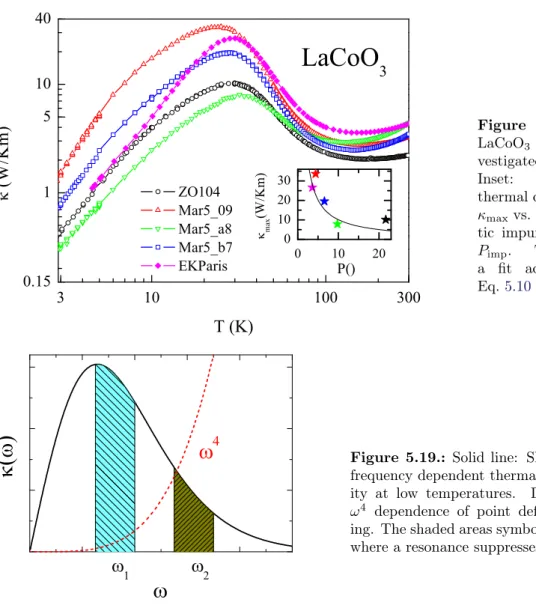
5.3.3. Impurity Contribution in LaCoO

. . . 75

5.4. Results . . . 79

5.4.1. LaCoO

. . . 79

5.4.2. RCoO

with R = La, Pr, Nd, and Eu . . . 80

5.4.3. RCoO

: Comparison to the Literature . . . 82

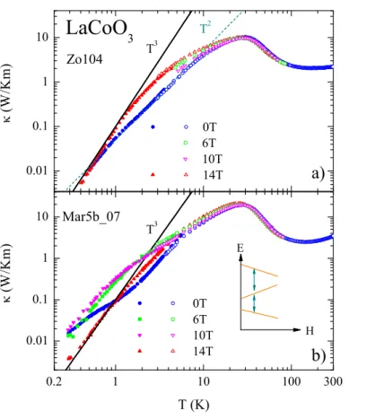
5.4.4. LaCoO

: Low Temperatures . . . 82

5.4.5. LaCoO

: Field Dependence of κ . . . 85

5.4.6. LaCoO

: Comparison Zero Field . . . 85

5.4.7. LaCoO

: Influence of the Spin-State Transition on κ . . . 88

5.4.8. RCoO

with R=Pr, Nd, and Eu: Low Temperatures . . . 95

5.4.9. PrCoO

and NdCoO

: Influence of the Spin-State Transition on κ . . . 95

5.4.10. Resonant Scattering in PrCoO

. . . 97

5.5. Conclusions . . . 99

6. Thermal Transport of La

Sr

CoO

and La

Eu

Sr

CoO

101 6.1. Introduction . . . 101

6.2. Samples . . . 102

6.3. Experimental Results . . . 103

6.4. La

Sr

CoO

. . . 103

6.4.1. Resistivity . . . 103

6.4.2. Thermal Conductivity . . . 104

6.4.3. Thermopower . . . 106

6.4.4. Figure of Merit . . . 109

Contents

6.5. La

Eu

Sr

CoO

. . . 109

6.6. Conclusions . . . 113

7. Thermal Conductivity of Orthorhombic Manganites 115 7.1. Orthorhombic RMnO

Perovskites . . . 115

7.2. Samples . . . 118

7.3. Thermal Conductivity of RMnO

: Overview . . . 118

7.4. NdMnO

. . . 120

7.4.1. Thermal Conductivity of NdMnO

: Zero Field . . . 121

7.4.2. Thermal Expansion of NdMnO

in Magnetic Fields . . . 122

7.4.3. Magnetostriction . . . 124

7.4.4. Analysis: Thermal Expansion and Susceptibility . . . 126

7.4.5. The Spin-Flop Transition . . . 133

7.4.6. Uniaxial Pressure Dependences . . . 134

7.4.7. Specific Heat . . . 135

7.4.8. Thermal Conductivity of NdMnO

: Scattering by Magnetic Excitations 136 7.4.9. Thermal Conductivity of NdMnO

: Influence of Magnetic Fields . . . . 138

7.5. TbMnO

. . . 139

7.5.1. Thermal Conductivity . . . 140

7.6. Conclusions . . . 144

8. Summary 145 A. Additional Measurements 149 A.1. TbMnO

. . . 149

A.2. GdMnO

. . . 157

A.3. GdFe

(BO

)

. . . 160

A.4. Bechgaard Salts . . . 163

A.5. Spin Ladders . . . 164

A.6. Ca

Co

O

. . . 165

A.7. LaCoO

. . . 166

List of Figures 169

List of Tables 171

Bibliography 173

Publikationsliste 189

Danksagung 191

Offizielle Erklärung 193

Zusammenfassung 195

Abstract 197

Lebenslauf 199

1. Introduction

Transition-metal oxides with perovskite- and related structures are well known for their un- usual physical properties arising from strong correlations. La

CuO

is a parent compound of high-temperature superconductors [1]. LaMnO

shows the colossal magnetoresistance upon doping [2]. In LaCoO

, the rare example of a temperature-induced spin-state transition is realized. The interpretation of the complex phenomena observed in these compounds is diffi- cult and often controversially discussed in the literature. A useful tool is to investigate, how the properties of the systems change, if the La ion is replaced by a smaller rare-earth ion.

The resulting structural changes often give additional information, since the key parameters determining the physical properties are tuned. The interpretation of the results obtained from these compounds is often complicated by the presence of the rare-earth 4f moments.

A key for the data interpretation is therefore a reliable distinction of the effects caused by the rare-earth ions and the transition-metal complex. Moreover, interactions between these different magnetic subsystems may lead to additional phenomena. The thermal conductivity of transition-metal oxides often reflects the complex properties of these systems. Frequently, unusual temperature- and magnetic-field dependences are observed. There are various reasons for these phenomena: In the quasi one-dimensional spin-ladder systems large contributions to the heat transport are caused by magnetic excitations [3, 4]. In magnetic systems with large spin-phonon coupling an unusual suppression of the thermal conductivity is observed [5]. The thermal conductivity is a powerful tool to investigate these phenomena arsing from phononic, electronic, and spin excitations and their interactions

The unusual behavior of the thermal conductivity of La

CuO

was discovered already more than one decade ago [6]. In this publication the possibility of a magnetic contribution to the heat transport was discussed. However, the mechanism of the heat transport in La

CuO

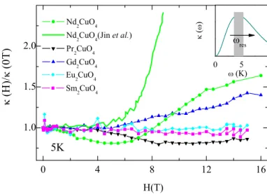
is still under debate [7–9]. One aim of the present work is to clarify this issue. Therefore, a systematic study of the thermal conductivity of the related rare-earth cuprates R

CuO

with R = La, Pr, Nd, Sm, Eu, and Gd will be presented. It will be shown that a magnetic contribution to the heat transport is a very fundamental property of the layered cuprates.

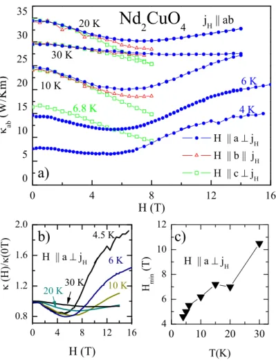
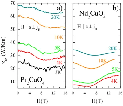
The results will be compared to one-dimensional systems, and the principal differences of the magnetic contribution to the heat transport between 1D and 2D will be discussed. Moreover, the low-temperature behavior under application of large magnetic fields will be addressed. It has been proposed in the literature that at low temperatures an additional magnetic contri- bution of Nd spin waves to the heat conductivity of Nd

CuO

is induced by the application of magnetic fields [10, 11]. The magnetic-field dependences of the thermal conductivity for the R

CuO

compounds will be presented. The analysis of the data gives new insight, since another mechanism causing the field-dependences is preferred.

The spin-state transition in LaCoO

is a long-standing issue in solid-state physics since the

1950’s. The question, whether a high-spin state or an intermediate spin-state is thermally

populated, is discussed controversially up to now. Whereas initially a high-spin state was

proposed, an intermediate-spin state scenario became popular during the last decade [12].

However, very recent results indicate that a high-spin scenario taking into account large spin- orbit coupling effects is a more appropriate description [13]. The thermal conductivity of LaCoO

has shown to be quite sensitive to the spin-state transition [9]. However, a quantita- tive analysis of this phenomenon lacks so far. This work presents a systematic study of the thermal conductivity on several LaCoO

single crystals, to obtain a clear picture of the intrin- sic features. A detailed quantitative treatment of the influence of the spin-state transition to the thermal conductivity is carried out. A consistent picture will be obtained, including the related compounds where La is replaced by the rare-earth ions Pr, Nd, or Eu. In addition, the reason for the observed complex field-dependent low-temperature behavior of the thermal conductivity will be clarified.

Upon charge-carrier doping the physical properties of LaCoO

substantially change. We present a systematic study of the thermal conductivity κ and the thermopower S of single crystals of La

Sr

CoO

with 0 ≤ x ≤ 0.3. For all Sr concentrations La

Sr

CoO

has rather low κ values, whereas S strongly changes as a function of x. We discuss the influence of the temperature- and the doping-induced spin-state transitions of the Co

ions on both, S and κ. From S, κ, and the electrical resistivity ρ we derive the thermoelectric figure of merit Z = S

/ κρ. A high figure of merit is a pre-condition for the applicability in thermoelectric devices. Moreover, the influence of an additional replacement of La by Eu is investigated.

The orthorhombic manganates RMnO

with R = La. . . Ho have attracted much interest, since in GdMnO

, TbMnO

, and DyMnO

ferroelectric ordering phenomena embedded in a magnetically ordered phase are observed[14, 15]. This phenomenon is often referred to as multiferroism. Since ferroelectricity is a structural phenomenon and therefore strongly coupled to the lattice, thermal conductivity is expected to be a useful probe to obtain new insights in the multiferroic properties of these compounds. This work presents thermal conductivity measurements of NdMnO

, GdMnO

, and TbMnO

. The experimental focus is a systematic investigation of the magnetic-field dependence of the heat transport by applying the field along the different crystallographic axes. In combination with thermal expansion and magnetization measurements it will be shown that resonant scattering by the 4f orbitals has, however, a much larger influence on the thermal conductivity, than the magnetic and electric ordering transitions at low temperatures.

This thesis is organized in the following way: In chapter 2, a brief introduction to the theoretical framework is given. Chapter 3 gives a description of the used setup and experi- mental methods. In chapter 4 a systematic study of the thermal conductivity of the rare-earth cuprates will be presented. Chapter 5 is devoted to the thermal conductivity of rare-earth cobaltates with spin-state transitions. Chapter 6 deals with the thermoelectric properties of Sr doped Cobaltates. The topic of chapter 7 is the heat transport in perovskite-type manganates.

In the appendix the results of additional measurements are documented.

2. Theory

In this chapter a brief introduction into the thermal conductivity and the thermopower of solids will be given. The focus will be to give an overview about conventional mechanisms established in the literature, and to quote some important basic relations. For a more detailed introduction see Refs. [16–20]. Finally, we will present a short introduction into the treatment of the 4f orbitals of the rare-earth ions in low-symmetry crystals.

2.1. Thermal Conductivity

In a crystal, the thermal conductivity is determined by heat carrying quasiparticles. The thermal conductivity κ can be generally expressed by the equation [16]:

κ = 1

d cv` (2.1)

where d denotes the dimensionality, c the specific heat, v the group velocity, and ` the mean free path of the respective heat carrying excitations. In most cases two kinds of excitations are responsible for the heat transport: phonons and electrons. The theoretical description is usually based on the Debye model in the first case, and on the electronic gas theory for the latter case.

2.1.1. Lattice Contribution

The heat carrying excitations in an insulating crystal lattice are phonons. For T Θ

, where Θ

denotes the Debye temperature, the specific heat can be calculated by the Debye formula [16]

c

= 3k

2π

v

k

~

T

Z

0

x

e

(e

− 1)

dx. (2.2)

Here, v is the sound velocity, which is identical to the group velocity in Eq. 2.1. The main problem in the calculation of the lattice contribution to κ is the estimation of the mean free path `. Three kind of scattering processes usually determine `, scattering of phonons by phonons, scattering by lattice imperfections, and scattering at the crystal surface.

At very low temperatures only the latter process is relevant. Then ` is given by a constant which is determined by the sample dimension L

. In this case

, it follows from Eqs. 2.1 and 2.2:

κ = 2 15 π

k

k

T

~

L

v

. (2.3)

According to Ref. [17], here the averaged sound velocity can be calculated via v = v

2( v

v

)

+ 1

/

2( v

v

)

+ 1

(2.4)

1At low temperatures the integrand gets small for large x. Therefore one sets ΘD/T → ∞ and uses R∞

0 x⁴e^x

(e^x−1)²dx= ^4π₁₅⁴.

1 10 100 10

100 1000

(W/Km)

T (K)

~T 3 LiF

(Berman et. al.)

NdGaO 3

(Schnelle e t al.) Fits

Figure 2.1.: Thermal conductivity of LiF (Berman et al. [21]) and NdGaO3

(Schnelle et al. [22]). Lines are fits by Eq. 2.5. The parameters were L = 7 (1)mm, Θ_D = 700(680)K, v = 6000 (4800)m/s, P = 0.07 (3.3) 10⁻⁴³s³, U = 2.2 (6.8) 10⁻¹⁸s, andu= 6(5.6) for LiF (NdGaO₃). [22,23].

from the measured longitudinal and transverse sound velocities v

and v

, respectively. In this limit the thermal conductivity follows the T

dependence of the specific heat. At high temperatures ` is mainly determined by Umklapp processes, which result from phonon-phonon interactions. Since at high temperatures the number of excited phonons is proportional to T,` ∼ 1/T follows. The specific heat becomes temperature independent for T → Θ

. Thus, κ ≈ 1/T follows at high temperatures.

2.1.2. Extended Debye Model

To describe the thermal conductivity more quantitatively, Eqs. 2.1 and 2.2 can be written as κ

= k

2π

v

k

~

T

Z

x

e

τ (ω, T )

(e

− 1)

dx (2.5)

where τ (ω, T ) = v/` is a temperature and frequency dependent scattering rate. Under the assumption that the different scattering processes act independently, one can write τ

as a sum of the different scattering rates:

τ

= τ

+ τ

+ τ

+ τ

+ . . . . (2.6) The used scattering rates have the following meanings:

• τ

= v/L: This is the boundary scattering term, which describes the reflection of phonons by the crystal surface.

• τ

= P ω

: This term describes point defect scattering, and is the most effective term in the temperature range, where the phononic maximum of κ occurs. At lower temperatures, phonons with larger wave length and therefore small ω are the dominant heat carriers, and τ

is less effective. The physical picture is, that the long wave length phonons do not ”see” the small point defects. At high temperatures τ

is less important, because Umklapp scattering is much more effective. In the data analysis we use P as an adjustable parameter describing the scattering strength.

• τ

= U T exp(Θ

/uT ). This term describes Umklapp scattering. The factor U gives

the scattering strength, the parameter u determines at which temperature Umklapp

scattering sets in.

2.1. Thermal Conductivity

• In some cases other scattering rates may be introduced, as e.g. scattering on planar de- fects τ

= Dω

, which is useful for systems with layered structures (e.g. the cuprates).

For a detailed survey of different scattering rates see e.g. Ref. [24].

To illustrate the data analysis by Eqs. 2.5 and 2.6, Fig. 2.1 shows literature data for LiF and, closer to the compounds investigated in this thesis, NdGaO

[21, 22]. The Debye temper- atures and sound velocities where taken from the literature [22, 23], and the other parameters were adjusted to the data. For LiF the general temperature dependence is modelled very well, particularly the low-temperature T

behavior. Around the maximum larger deviations between the fit and the data are observed, which come from the oversimplification of the used scattering terms. In NdGaO

the temperature dependence above the maximum is modeled well, but the fit is much too high for lower temperatures. Here, additional scattering mecha- nisms, like e.g. scattering on spin waves, paramagnetic impurities, etc. play also a role, which are not included in Eq. 2.6.

2.1.3. Electronic Contribution

Electrons carry a specific heat which is proportional to k

T . Eq. 2.1 is valid for electronic heat transport, too. Here, the Fermi velocity v

is used for the velocity of the electrons, which yields [16]

κ

= π

nk

T ` 3mv

. (2.7)

Here, n is the electron density and m the electron mass. Because the electron carries charge and heat simultaneously, usually the Wiedemann-Franz law holds, which connects electrical and thermal conductivity:

κ = LσT, (2.8)

where L denotes the Lorenz number. The free electron gas theory yields the value L

= 2.45 · 10

W/ΩK

. The Wiedemann-Franz law is valid, if only elastic scattering processes occur, which is usually the case for low temperatures (only boundary scattering) and for high temperatures. For intermediate temperatures charge carriers are mainly scattered by phonons which lowers the value of L.

In good metals, only the electronic contribution to κ is relevant. The reason is that the absolute values of κ

are large, and that phonons are strongly scattered by the electrons. For bad metals electronic and phononic contributions can be of the same size. For bad insulators often only the phononic contribution is relevant at low temperatures, but through the thermal activation of electrons the electronic contribution becomes more and more important for high temperatures.

2.1.4. Other Contributions to κ

In principle, every quasiparticle carrying specific heat and a non-vanishing group velocity

can contribute to the heat transport. Often, the latter condition is the limiting factor, as it

is e.g. the case for optical phonons which have only a small dispersion. Furthermore, the

additional quasiparticles can scatter phonons, or are scattered by phonons, which may even

overcompensate the additional contribution to the heat transport.

0 4 8

=7

=3

()

=0.5

()

Figure 2.2.:Frequency dependent ther- mal conductivity without resonant scat- tering or∆ = 0(dashed line) and for res- onant scattering with different level spac- ings∆(solid lines). Inset: Sketch of the resulting thermal conductivityκ(∆).

2.1.5. Minimum Thermal Conductivity

In the Debye model discussed above, ` is not limited to a lowest value, and the 1/T behavior of κ continues up to highest temperatures. In reality, however, the interatomic distances give a lower limit to `. It follows, that κ will not drop below a minimum value κ

. In this limit, the concept of well defined phonons is no longer a good approximation, and therefore other treatments of the minimum thermal conductivity were carried out in the literature. In Ref. [25] the authors discuss a model originally based on Einstein, which uses coupled local oscillators to describe κ. The physical picture is that the energy makes ”random walks”, with energy exchange between nearest and next-nearest neighbors. This treatment results in

κ

= π 6

k

n

X

i

v

T

Θ

Z

0

x

e

(e

− 1)

dx, (2.9) where n = N/V denotes the atomic density and i sums up the different polarizations. The Debye temperatures Θ

for the different polarization directions i are given by

Θ

= (~v

/k

)(6π

n)

. (2.10) The comparison of the calculated values κ

to the measured κ at high temperatures yields an underestimation of κ

up to a factor of 2 [25]. The minimum thermal conductivity can be taken into account in Eq. 2.5 by introducing a minimum mean free path `

, and replacing τ (ω, T ) by max{τ

(ω, T ), l

/v

}.

2.1.6. Resonant Phonon Scattering

Resonant scattering processes can further suppress the phononic heat transport, in addition

to the already discussed mechanisms. For resonant processes a two (or multi) -level system is

necessary. The idea is that a phonon with an energy exactly equal to the level splitting ∆ is

absorbed by stimulating a transition, and later on it is remitted. This process is also possible

for the excited state, then a de-excitation process absorbs the incoming phonon. Because the

direction of the re-emitted phonon is not correlated to the absorbed phonon, both processes

suppress the heat transport. A quantum mechanical treatment of this mechanism [27] gives

2.1. Thermal Conductivity

Figure 2.3.: Left panel: Thermal resistance W = 1/κ for Holmium ethylsulfate at Helium temperature. The data are taken from Ref. [26]. Right panel: Level scheme of the paramagnetic impurities in Holmium ethylsulfate. The upper level is a singlet and the lower level a doublet which splits in a magnetic field due to the Zeeman effect.

the scattering rate of such a resonant scattering process:

τ

= R 4ω

∆

(∆

− ω

)

· (N

+ N

) . (2.11) Here, R gives the overall coupling strength, ∆ the energy splitting and N

and N

the popu- lation factors of the resonating levels. For a two-level system it directly follows N

+ N

= 1, which means that τ

becomes temperature independent. The effect of Eq. 2.11 is illustrated in Fig. 2.2. The ω dependent thermal conductivity is 0 for ω = 0 and for ω → ∞, and shows a maximum inbetween. The resonance term is effective in a narrow frequency range.

Fig 2.2 illustrates the influence of a resonant process for the case of a two level system, with

an increasing gap ∆. For ∆ = 0 no resonance occurs, and with increasing ∆ the resonance

suppresses κ(ω), leading to a suppression of κ(∆) (see inset). If ∆ reaches the maximum

of κ(ω) the suppression is most effective again, and for further increasing ∆ the resonance

becomes less effective, and κ(∆) increases again. There are various possible origins of the

resonance processes. In Refs. [27, 28] a double-peak structure of κ in SrCu

(BO

)

could be

successfully explained by resonant scattering of phonons by magnetic excitations. Another

frequent source of resonances is the presence of paramagnetic impurity levels [26, 29, 30]. A

prominent example in this context is holmium ethylsulphate [26]. Fig. 2.3 shows the thermal

resistance (1/κ) of holmium ethylsulphate at 4.25 K in magnetic fields up to 5.3 T. A strong

nonmonotonic field dependence is observed. The resonant process is caused by phonons induc-

ing transitions of the paramagnetic ions. The level scheme of holmium ethylsulphate contains

a singlet and a doublet, the latter splits in a magnetic field by the Zeeman effect. Because of

the four different transitions, which all have a field-dependent energy gap, the complex field

dependence of κ arises. Note, that Eq. 2.11 describes only the simplest case of a so-called

direct resonance process. Processes of higher order, where e.g. two phonons are involved, an

inelastic processes, where incoming and outcoming phonons have different energies, are also

possible [31].

2.2. Thermopower

The thermopower S is defined by

S = E ~

∇T (2.12)

and describes the electrical field

caused by a heat gradient, with the additional condition that no electrical current is allowed to flow. This effect can be reverted. The generation of a heat gradient by an electrical current is called Peltier effect. The Peltier constant Π and the thermopower S are connected via the Onsager relation

Π = ST. (2.13)

A simple picture of the thermopower in metals can be given as follows: In principle, electrons and holes contribute to charge transport. First, we regard only electrons. If a temperature gradient is applied along the sample, the electrons are faster in the hot side of the sample.

Therefore, electrons coming from the hot side of the sample have a larger velocity, which causes an electron diffusion from the hot side to the cold side. Since no current flows, a voltage is generated which leads to a steady state.

If electrons and holes are present, the thermovoltage would vanish, if both types of charge carriers move in the same way. This is not the case in reality because of the different mobilities of the quasiparticles. For metals an estimation of the thermopower can be given by

S

= − π

k

T 3q

∂(ln σ(E))

∂E

E=EF

(2.14) where σ(E) is the electrical conductivity [32]. The thermopower vanishes for T → 0, which follows from the vanishing of the entropy according to the third law of thermodynamics. A complication occurs, since the mean free path is generally energy dependent, which causes a different scattering for the electrons coming from the hot end of the sample compared to the electrons with the opposite direction. The energy dependence of the mean free path is not known well in general, and can cause a complex behavior of S. At low temperatures a further effect becomes important: the phonon drag. The considerations above assume random scattering centers for the electrons. In fact, the temperature gradient over the sample leads to a phonon flow from the hot end to the cold end of the sample, because in the hot end more phonons are excited. Although the phonons itself do not contribute to the thermopower, they can ”drag” charge carriers by the phonon-electron interaction, and enhance the thermopower in this way. At high temperatures this effect is negligible, because phonon-phonon interaction dominates.

The measurement of the thermopower is not straightforward, since the usual setup (see Chp. 3) always measures the sum of the thermopower of the sample and the wires used to measure the voltage:

S

= S

− S

(2.15)

Note, that the thermopower of the wires has a negative sign (see e.g. Ref. [33]. At low temperatures one can avoid this problem by the use of superconducting wires, which have a vanishing thermopower. It is, however, possible to measure the absolute S directly by the use

2E~=E~+ (1/e)∇µ~ is the sum of the electrostatic fieldE~ and the gradient of the chemical potentialµ[32].

2.3. Figure of Merit

of the Thompson effect [18]. Herefore, the heating power of a wire is measured, with a heat current and a electrical current applied at the same time. The heating power is given by [32]:

P = dq

dt ρj

+ dκ

dT (∇T )

− T dS

dT (∇T ) · j (2.16)

The Thompson heating of the wire can be distinguished from Joule heating, since it changes sign, if the sign of the electrical current is changed. Since only the derivative of S is determined, one has to integrate dS/dT and to measure one absolute value to obtain the integration constant. This can be done at low temperatures by the use of superconducting wires. This method is complex, and has to be performed very accurately, since the integration of dS/dT is very sensitive to measurement uncertainties. Therefore one usually uses the literature data for the thermopower of Pb estimated by this method in the literature, and calibrates the used wires against Pb [18]. For a detailed introduction to the thermopower I refer to Refs. [18–20]

2.3. Figure of Merit

The thermoelectric figure of merit ZT gives a measure for the efficiency of a material for thermoelectric cooling. A simple derivation can be given as follows: A thermoelectric cooler transports heat from a cold to a hot reservoir. The total heat removal rate is given by [19]

q

= ST

I − 1

2 I

R − K∆T, (2.17)

where S is the thermopower, T

the temperature of the cold reservoir, I the current, R = ρl/A the resistivity, K = κA/l the thermal conductance, and ∆T the temperature difference between the two reservoirs. The first term of Eq. 2.17 is the heat flow caused by the Peltier effect. The second term is the Joule heating, which has a negative sign, since it warms the cold reservoir. The factor 1/2 comes from the fact that one half of the heat flows to the warm reservoir. The third term describes the zero-current heat transport, which is determind by the thermal conductivity, and also counteracts the Peltier effect. From Eq. 2.17 it is directly clear that S has to be maximized, and κ and ρ to be minimized to obtain a high efficiency.

Furthermore, an optimal current can be obtained by resolving Eq. 2.17 with respect to ∆T (I ) and calculating the maximum value

∆T (I )

=

(ST)² 2R

− q

K (2.18)

with the optimum current I = ST /R. Finally one obtains from Eq. 2.18 the relation q

∼ S

KR (2.19)

which motivates the definition of the dimensionless figure merit ZT = S

T

κρ . (2.20)

For a more detailed introduction into the efficiency of thermoelectric devices, see Ref. [19].

L=5, S=1

. . . el-el

(F

, F

, F

, F

)

J=4 J=5 J=6

SO ζ

(33) (91)

(9) (11) (13)

Cf A

Cubic Tetr. lower

(n) = degeneracy

4f

Figure 2.4.: Schematic level splittings of a 4f² system due to electron-electron repulsion, spin-orbit (SO) coupling and crystal field (CF). Note, that the order of the levels of the split J = 4multiplet in the crystal field is exemplary.

2.4. 4f Orbitals in the Crystal Field

The dimension D of the Hamiltonian of a f

level system is given by

, which can reach values up to D = 4004 for n = 7. This means also a degeneracy D of the energy levels without any interaction. In a crystal (without magnetic field) the Hamiltonian consists of three parts,

H = H

+ H

+ H

. (2.21)

The first two terms are the same as for a free ion and describe the electron-electron interaction and the spin-orbit (SO) coupling. The third term gives the influence of the crystal field. The el-el interaction is usually described by Slater integrals A

, and the SO coupling by the energy ζ . In most cases the relation F

(> 5eV) ζ(≈ 0.1eV) E

(≈ meV) holds, which allows to take into account only a small sub-space of the original Hamiltonian. This is illustrated for a 4f

system in Fig. 2.4. Without interaction, one starts with 91 degenerate levels. The dominant energy scale of the el-el interaction gives a S = 1, L = 5 state according to Hunds rules, with 11 × 3 = 33 degenerate energy levels. If SO coupling is turned on, the levels further split into three levels with J = 4, 5, 6. The level spacing between the J = 4 and J = 5 state

is ≈ 0.3 eV≈ 3000 K, and usually only the lowest

H

state has to be taken into account. However, in many systems (e.g. Sm

) the higher multiplets are important, too.

In a crystal, the ligand-field further splits the

H

multiplet. The energy scales are hereby much smaller than in the d systems, since the 4f states are highly screened. The crystal field Hamilton can be written as [34]:

H

= X

m m

X

k=−m

A

C

, k, m = 0, 2, 4, 6 (2.22) with the crystal field parameters A

and the tensor operators C

. The parameters A

can be complex for m 6= 0, further the relation A

= (−1

)(A

)

generally holds. For higher

3Calculated for a Pr³⁺ion.

2.4. 4f Orbitals in the Crystal Field

symmetries most of the parameters A

vanish, or depend on each other. For the cubic O

symmetry 2 independent energies remain. In the tetragonal D

symmetry one has to deal with 5 and for the orthorhombic C

symmetry with 15 independent parameters. The splitting of the ground state multiplet is different for systems with odd and with even 2J . If 2J is odd, the Kramer’s degeneracy tells, that the J multiplets splits into quartets and doublets. In the lowest symmetry only doublets are realized. If 2J is even, the multiplet splits into singlets, doublets and triplets. Here, only singlets are realized for the lowest symmetry. For a given 4f

system and a given symmetry one can determine the principle splitting of the ground state multiplet. Tab. 2.2 shows these results for the rare earth ions R

[35]. Note, that these results reflect only the symmetry of the system, and give no information about the order of the different levels.

The data analysis was performed with the Mathematica

package ”CrystalFieldTheory”

(CFT) developed by M. Haverkort [36]. This package solves the Hamiltonian Eq. 2.21 by exact diagonalization of the full multiplet. The used Slater integrals F

and the SO coupling constant ζ obtained from Hartree-Fock calculations by M. Haverkort are listed in Tab. 2.3.

The crystal field is usually investigated by neutron scattering. These measurements yield the level scheme, since the transitions between different CF levels are measured. To get the parameters A

, a CF model has to be used and the A

values are usually fitted to obtain the best description of the energy level scheme. Here, the analysis is often simplified by only taking the ground state multiplet into account. In this case, so-called Stevens operators are frequently used, which yield a different parameterization of the CF Hamiltonian. The conversion of the parameters of the Stevens formalism to the A

parameters is complex in lower symmetry systems.

In this work, tetragonal and orthorhombic systems with R

ions were investigated. The crystal field was studied in detail in the literature for the tetragonal cuprates, which will be discussed in more detail in Chp. 4.

2.4.1. Orthorhombic Perovskites

In the orthorhombic perovskites one has to deal with 15 independent CF parameters, but usually only a few energy levels are present for the fitting of the A

values. Therefore, usually additional assumptions are made in the data analysis, which restrict the number of free parameters (see e.g. Refs. [37, 38]). To my knowledge no systematic crystal field investigations of orthorhombic cobaltates and manganates are available

. However, such investigations have been made for related compounds RM O

, with R = Pr, Nd, and Eu; and M =Al, Ga, Fe, and Ni. The structural distortions are similar in these compounds, which leads to similar CF effects for the same R and different M . We will explore this for the comparison of the available data of CF splitting energies for various PrMO

and NdM O

compounds.

In PrM O

, the

H

multiplet of the Pr

ion splits into 9 singlets (see Tab. 2.3). The measured crystal-field splitting is indeed very similar for different orthorhombic PrM O

com- pounds. In Tab. 2.1 the energy levels for various PrMO

compounds measured by neutron scattering experiments are listed. Note, that because of the different sizes of the scattering cross section, only 5 or 6 energies can be resolved. According to Tab. 2.1, the energies E

to E

are almost identical for M =Fe, Ga and Ni. Larger differences mainly occur for the first

4Mathematica 5.2, Wolfram Research.

5In Ref. [39] the authors observe some CF excitations in their investigation of the spin-wave spectrum of TbMnO3 and PrMnO3.

excited level, the energy E

ranges from 23 K to 74 K. To resolve this issue, the M-O-M bond angle is also listed in Tab. 2.1. This parameter is useful to characterize the distortion (see also Chp. 7). From the comparison with E

a direct correlation can be made, E

increases with increasing bond angle M -O-M . This systematic also holds for PrCoO

and PrMnO

, where the energies of the first (second) excited level is known from other measurements, see Tab. 2.1.

In NdMO

, the

H

multiplet of Nd

splits into 5 doublets. Here, all transitions are observed, and the energy splitting is very similar for the different compounds, too. The smaller value of E

in NdFeO

may indicate a similar dependence on the M-O-M angle as in PrMO

, but this is not clear from the available data. No direct information of the level schemes of NdCoO

and NdMnO

is available.

2.4.2. Specific Heat and Susceptibility

From the eigensystem calculated from Eq. 2.21 the specific heat and the magnetic susceptibility of the 4f

system is calculated straightforwardly:

C

(T ) = ∂

∂E P

n=1

E

exp(−

BT

)

Z (2.23)

with

Z =

Di

X

n=1

exp(− E

k

T ). (2.24)

and

χ(T, H) = M (T, H )

H =

P

n=1

M

(H) exp(−

BT

)

ZH (2.25)

with

M

(H) = hn|(L

+ 2S

)|ni. (2.26)

Note, that usually the specific heat is much less sensitive to the CF, since here only the energies

are relevant.

2.4. 4f Orbitals in the Crystal Field

R

M -O-M E

E

E

E

E

E

Ref.

(Å) (

) (K) (K) (K) (K) (K) (K)

PrFeO

0.645 152 [40] 23 171 270 418 673 [41]

PrGaO

0.62 154 [42] 55 171 232 429 754 [41]

PrGaO

59 186 249 441 777 908 [38]

PrNiO

0.56 159 [43] 74 174 235 440 696 [44]

PrCoO

0.545 159 [45] 70 ∗ PrMnO

0.645 150 19 †

PrMnO

20 ‡ 185 ‡

NdGaO

0.62 153 [46] 132 261 611 789 [47]

NdGaO

153 132 262 606 788 [48]

NdFeO

0.645 151 [49] 120 263 526 705 [37, 50]

NdNiO

0.56 156 [51] 129 220 765 835 [44]

NdCoO

0.545 156 [52]

NdMnO

0.645 150 [53]

Table 2.1.: Ionic radiiM [54], M-O-M bond angles, and crystal field energies of PrMO₃and NdMO3. *) Value estimated by thermal expansion, see Sec. 5.4.10. †) Value estimated by specific heat [55]. ‡) Value estimated by neutron scattering from Ref. [39].

R

S L J GS D d

d

d

d

sg db tr qt sg db sg db

Ce 1/2 3 5/2

F

14 6 1 1 3 3

Pr 1 5 4

H

91 9 1 1 2 5 2 9

Nd 3/2 6 9/2

I

364 10 1 2 5 5

P m 2 6 4

I

1001 9 1 1 2 5 2 9

Sm 5/2 5 5/2

H

2002 6 1 1 3 3

Eu 3 3 0

F

3003 1 1 1 1

Gd 7/2 0 7/2

S

3432 8 2 1 4 4

Tb 3 3 6

F

3003 13 2 1 3 7 3 13

Dy 5/2 5 15/2

H

2002 16 2 3 8 8

Ho 2 6 8

I

1001 17 1 2 4 9 4 17

Er 3/2 6 15/2

I

364 16 2 3 8 8

Tm 1 5 6

H

91 13 2 1 3 7 3 13

Yb 1/2 3 7/2

F

14 8 2 1 4 4

Table 2.2.: S, L, J, ground state multiplet (GS), dimensionality of the full multiplet D, degeneracies of the ground multiplet for the free ion, cubic, tetragonal, and lower symmetry (sg: singlet, db: doublet, tr: triplet, qt: quartet) [35].

Atom# Atom Conf r

r

r

ζ F

F

F

F

R

(Å

) (Å

) (Å

) (eV) (eV) (eV) (eV) (eV)

58 Ce 4f

0.367 0.312 1.208 0.087 0.000 0.000 0.000 0.000

59 Pr 4f

0.337 0.265 1.230 0.102 25.711 12.221 7.666 5.515

60 Nd 4f

0.312 0.229 1.252 0.119 26.739 12.719 7.981 5.742

61 P m 4f

0.291 0.200 1.274 0.136 27.719 13.191 8.278 5.956

62 Sm 4f

0.273 0.177 1.296 0.155 28.665 13.643 8.562 6.161

63 Eu 4f

0.257 0.158 1.318 0.175 29.581 14.079 8.836 6.357

64 Gd 4f

0.243 0.143 1.339 0.197 30.474 14.501 9.100 6.548

65 Tb 4f

0.230 0.129 1.361 0.221 31.344 14.911 9.357 6.732

66 Dy 4f

0.219 0.118 1.383 0.246 32.200 15.312 9.608 6.912

67 Ho 4f

0.208 0.108 1.405 0.273 33.040 15.704 9.853 7.088

68 Er 4f

0.199 0.099 1.427 0.302 33.865 16.089 10.093 7.260

69 Tm 4f

0.190 0.092 1.449 0.333 34.679 16.467 10.328 7.429

70 Yb 4f

0.182 0.085 1.471 0.366 35.483 16.839 10.560 7.596

3. Experimental

In this section the used experimental methods will be introduced. The general setup will be discussed only briefly, since it is the same as used in Ref. [57], where a detailed description is given. Extensions of the setup, as the use of a new sample holder for measurements of κ down to 250 mK in a

He system, will be described in more detail. Furthermore, test measurements to check the used thermocouple calibration will be presented.

3.1. Measurement of Transport Properties

In this thesis measurements of thermal conductivity, thermopower, and resistivity were per- formed. Generally, transport measurements are done providing an external perturbation to the sample and measuring the response of the sample. In our case, the external perturbation is either an electrical current, or a heat supply. The response is either an electrical voltage or a heat gradient over the sample. Here, only longitudinal effects are regarded, so the response of the samples is measured in the same spacial direction as the perturbation.

3.1.1. Experimental Framework

The main purpose of the experimental setup is to provide the desired control parameters, as pressure, temperature and magnetic field. Here, pressure is no adjustable control parameter

. The temperature / the magnetic field is usually either kept fixed, or changed with a constant rate. The control of the magnetic field is in principle easy, since it is based on the control of electrical currents, and so static magnetic fields, or magnetic field sweeps are possible simply by giving the magnet power supply the right commands (within the limits given by the used magnet and magnet control system). No further measurement of the field is necessary. In contrast, the temperature needs a control loop, usually realized by a temperature controller using a PID algorithm. This requires the measurement of the temperature, and for measure- ments with fixed temperature it has to be checked, if the temperature is stable enough. For temperature sweeps, a stabilization is only needed for the starting value, a constant rate is then achieved by the controller.

One can group the measurements in those where the data points are taken with fixed tem- perature and magnetic field, and those where one of these quantities is continuously changed during the measurement.

3.1.2. Measurements with fixed Temperature and Field

Thermal conductivity is usually measured with fixed temperature and field. The procedure is here as follows: First, the required magnetic field and temperature are set, with the external

1Resistivity measurements are usually done in a gas atmosphere, since here no vacuum is needed, and a faster temperature control and a better thermalization of the sample is possible. The influence of the atmospheric pressure is, however, negligible.

perturbation of the sample (sample heater) turned off. Then it is waited until certain stability criteria are fullfilled, while data points are continuously taken. This is achieved by taking the last n (usually n = 150) points and calculating the average, the slope, and the standard deviation. For the measurement signal(s) the slope and the standard deviation are checked, for the temperature additionally the set point deviation. If all criteria are fullfilled, average values of all measured quantities are calculated over the n points. Then the sample heater is turned on, and again it is waited for all stabilization criteria to be fullfilled, yielding a second set of values. From the two sets one can calculate the measured quantities, either by averaging both values (temperature) or by taking the difference. The latter procedure eliminates the offset values, which are always present due to thermovoltages in the wiring and in the plug connections. This is especially important for the low-voltage signals, as the thermocouple voltage. This procedure is basically the same for all measurements with fixed temperatures and fields. Resistivity could be performed in the same way, however a factor of

√ 2 in the resolution can be gained if the current is switched between positive and negative values, instead of just turning it off.

3.1.3. Measurements with Temperatures and Field Sweeps

The disadvantage of measurements with fixed temperature and field is, that they are very time consuming. An accurate temperature stabilization can take a lot of time. Furthermore, only a small amount of the measurement time is used to take actual data points. Therefore it is desirable to stabilize only temperature or field, and to sweep the other quantity with a constant rate, taking the measured values continuously. This requires that the response time of the sample is not too slow and that the correction of offset values is still possible. Therefore the offset values should not change too fast as a function of temperature / magnetic field. For the regarded transport properties, this requirements are usually only fullfilled for resistivity measurements. Here, the offsets can be either neglected (insulators), or are taken into account be changing the sign of the current periodically in blocks of typically 10 − 20 s [33].

3.1.4. Probes

For the thermal transport properties six basically identical probes are available, which allow measurements between room temperature and ≈ 5 K. The lowest achievable temperature can be improved to ≈ 2.5 . . . 3 K by pumping on the lambda plate. The probes are described in detail in Ref. [57]. For the resistivity measurements either a quick measurement device [33], or a variable temperature insert was used. For the latter a new probe was built up which covers the temperature range of 1.5 − 300 K and allows the measurement of two samples simultaneously.

3.2. Thermal Conductivity

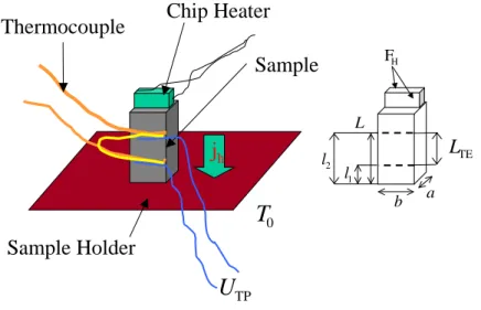
The setup used for the thermal conductivity measurements is sketched in Fig. 3.1. The sample

holder is kept on a temperature T

. A chip heater is mounted on the top of the sample, which

can produce a heat gradient over the sample. This heat gradient is measured by a thermocouple

attached to the sample. The thermal conductivity is calculated with the following equation

3.2. Thermal Conductivity

Sample Holder

Chip Heater Thermocouple

Sample

j

T

U

L

FH

l1

l2

L

b a

Figure 3.1.: Left: Setup for thermal conductivity measurements. Right: geometry used for the estimation of the radiation losses.

[57]:

κ = U

· I

· S(T, B)

∆U

l

A . (3.1)

Here, U

denotes the Voltage of the sample heater, I

the current of the sample heater, S(T, B) the temperature and field dependent calibration curve of the thermocouple, U

the voltage of the thermocouple, l the distance between the thermocouple ends, and A the cross section of the sample. S(T, B) was determined carefully in Ref. [57], and checked with several reference samples, see Sec. 3.6.1. The used thermocouples were in most cases Chromel-Au+0.07%Fe, which are perferably used at low temperatures, and in some cases Constantan-Chromel, which have a higher sensitivity at high temperatures.

3.2.1. Error Sources

Whereas the voltage and current measurements are very precisely, the determination of the geometric factors l and A is affected by a large error of ≈ 5 − 20%, depending on the sample geometry. This can be neglected in most cases, since the qualitative behavior of the curves is not affected. Furthermore, the thermopower of the used thermocouples gives an error up to 5%, see Sec. 3.6.1. More crucial are, however, systematic errors which can cause large effects.

These are mainly caused by thermal shortcuts by the wiring, or by radiation losses at high

temperatures. Both effects are discussed in detail in Ref. [57]. The error through thermal

shortcuts can be minimized by the use of proper wiring, in most cases manganin wires by a

diameter of 50 µm. For the measured samples in this thesis the influence of thermal shortcuts

has been carefully checked and can be neglected in all cases. Radiation losses depend on the

thermal conductivity of the samples and the geometry, and are usually large for samples with

a small κ and a large ratio of sample length and cross section, L/A. The latter parameters

are often restricted, and therefore radiation losses are often not to avoid. An estimation of

the radiation losses was e.g. done in [58]. In this reference only the sample surface and the

heater surface are taken into account. However, this is not sufficient because the wiring is a