A Polynomial Translation of Mobile Ambients into Safe Petri Nets

A Polynomial Translation of Mobile Ambients into Safe Petri Nets

Masterarbeit

am Fachbereich Informatik der TU Kaiserslautern

Susanne Göbel

Keywords: Mobile Ambient, Safe Petri net, model checking, reachability

Abstract. Mobile Ambients [CG98] are a modeling tech-

nique suitable to express typical network components and their

behaviour e.g. processes passing firewalls. We derive a decidable

subclass of the MA calculus by a translation into Safe Petri

nets. Our translation extends to arbitrary MA processes but

finiteness of the net and therefore decidability of reachability is

only guaranteed for processes bounded in depth and breadth.

Hiermit erkläre ich an Eides statt, dass ich die vorliegende Arbeit selbstständig verfasst und keine anderen als die angegebenen Quellen und Hilfsmittel benutzt habe.

(Ort, Datum) (Unterschrift)

Autorin: Bc. Sc. Susanne Göbel Email-Adresse: s_goebel@informatik.uni-kl.de Fachbereich: Informatik

Universität: Technische Universität Kaiserslautern Studiengang: Master Informatik

Erstgutachter: Dipl. Inf. Reiner Hüchting Zweitgutachter: Jun.-Prof. Dr. Roland Meyer

Zusammenfassung Typische Komponenten von Netzwerken und Net- zwerkverhalten, z.B. Prozesse, die Firewalls passieren, lassen sich gut in Mobile Ambients (MA) [CG98] modellieren. Durch Übersetzung in sichere Petrinetze ergibt sich hier eine entscheidbare Teilklasse der MA Prozesse.

Die Übersetzung selbst funktioniert für beliebige Prozesse, ein endliches

Netz und damit ein entscheidbares Erreichbarkeitsproblem ergibt sich aber

nur für Prozesse, die tiefen- und breitenbeschränkt sind.

Vielen Dank. . .

. . . möchte ich zunächst meinen beiden Betreuern Roland Meyer und Reiner Hüchting sagen, für Betreuung und Unterstützung, die schon lange vor dieser Arbeit begonnen hat und sich hoffentlich auch noch lange fortsetzen wird. Ihr habt mir ein faszinierendes Feld der Informatik erschlossen, dass mich hoffentlich irgendwann ernähren, auf jeden Fall aber nie loslassen wird.

Mit der Masterarbeit schließt sich ein spannendes Lebenskapitel: Mein Studium.

Ich habe Freiheit in einem Maß erfahren, dass ich vorher kaum für möglich gehalten hätte, aber auch Heimweh und Verlorensein. Ich danke meinen Eltern und Großeltern für Geborgenheit und einen Ort, an den ich bis heute fliehen kann, wenn mir alles zuviel wird. Ihr habt mir mein Studium ermöglicht und ihr seid bis heute für mich da, wenn ich Sorgen habe.

Genauso begleitet haben mich Freundinnen, die schon in der Schulzeit an meiner Seite waren und bis heute sind: Sonja, die vom Kindergarten bis als Trauzeugin mit mir gegangen ist, Mara, die mit mir die Männerwelt unsicher gemacht hat und bei Liebeskummer immer eine zuverlässige Anlaufstelle war, Marina, die mich nicht erst, aber vor allem in meiner Schwangerschaft so kompetent und mitfühlend begleitet hat und bestimmt mal eine tolle Ärztin wird, Kristina, mit der man schon immer wunderbar träumen und spielen konnte, und schließlich Vali, die alle Sorgen einfach weglacht. Noch länger mit mir geht meine Schwester – wir haben uns gemeinsam durch Pubertät und Schule gekämpft und so viel zusammen erlebt, wie man das wohl nur als Geschwister kann. So verschieden sich unsere Leben entwickelt haben, das Band ist doch nie ganz abgerissen und ich bin unglaublich stolz und glücklich, euch alle zu haben – ich hab euch lieb.

Während des Studiums habe ich neue Freunde gefunden, auch wenn die erste Clique nicht gehalten hat, bin ich doch euch allen dankbar für die gemeinsame Zeit. Viele sind geblieben und sind zu wichtigen RatgeberInnen, LeidensgenossInnen und in Helens Fall sogar beinahe zu einem Familienmitglied geworden. Da sind noch Anne, Frank, Laura und Stephan, Lars, Marco, Christian, Roya und Christina. Mit manchen kann man schwimmen gehen, mit manchen wandern, Brettspiele spielen oder Musik machen, aber mit allen kann man reden.

Ebenfalls dankbar bin ich der Studienstiftung und Professor Liggesmeyer, der mich im zweiten Semester vorgeschlagen hat. Ich habe durch sie den Zugang zu einem Gesellschaftsbereich erhalten, der sich sicherlich im Berufsleben als hilfreich erweisen wird. Dem gesamten Fachbereich, vor allem der Fachschaft und den Gremien danke ich für unsere gemeinsame Zeit und Arbeit. Ich denke wir haben viel bewegt und ich bin sicher, ich habe viel gelernt.

Ganz neben der Uni und dennoch eng damit verwoben ist mein Mann Chris, der

seit drei Jahren mit mir durch dick und dünn geht. Für eine Ehe, die so ist, wie sie

sein sollte, weil sie uns beide trägt und stützt, für eine Schulter, an die ich mich immer

lehnen kann, auch wenn sie eher spitz und etwas härter ist, möchte ich dir aus tiefstem

Herzen danken. Du hast dich begeistert mit mir in das Abenteuer Familie gestürzt

und bist so liebevoll und fürsorglich bisher für mich und jetzt für Katharina und mich da.

Schließlich sind da noch Mady und Katharinas Patentante Nathalie, die uns durch die schwere Zeit des Krankenhauses begleitet haben und hoffentlich auch weiterhin als selbstgewählte Familie mit uns zusammenstehen.

Und dann, ja dann ist da natürlich noch die kleine Katharina selbst, die nicht erst

seit dem 20.8.2013 unser Leben ordentlich durcheinanderwirbelt. Ich danke dir fürs

Kuscheln, für dein Lächeln und das unfassbare Vertrauen, das aus deinen großen

blauen Augen spricht. Du bist so ruhig und friedlich, dass ich die letzten Kapitel

fertigstellen konnte, als du schon in meinen Armen lagst.

Contents

1 Introduction and Related Work 6

1.1 Overview . . . . 7

2 Preliminaries 9 2.1 Safe Petri Nets . . . . 9

2.2 Mobile Ambients . . . . 10

2.3 Bisimulations . . . . 12

3 Translating MA Processes into Safe Petri Nets – The Idea 15 3.1 Translating MA Terms into Safe Petri Net Markings . . . . 15

3.2 Translating Capability Actions into Petri Net Transitions . . . . 17

3.3 Managing Names in the Petri Net . . . . 22

3.4 Guaranteeing Finiteness . . . . 30

4 From MA to rMA 32 4.1 Preprocessing . . . . 32

4.2 The Refined MA Calculus . . . . 33

4.3 Bisimulation between MA and rMA . . . . 33

5 The Construction: MA-PN 35 5.1 Places . . . . 35

5.2 Transitions . . . . 38

6 From rMA to MA-PN 50 6.1 Stable MA-PN Markings Maintain a Tree Structure . . . . 50

6.2 Connecting rMA and MA-PN . . . . 54

6.3 Bisimulation between rMA and MA-PN . . . . 64

7 Extensions and Optimisation 66 7.1 Saving Transitions by Modularisation . . . . 66

7.2 Excluding Public Names from Parameter Lists . . . . 66

7.3 Relaxed MA Semantics . . . . 67

7.4 Simulation of Unbounded Processes . . . . 69

8 Conclusion and Future Work 73 A Polynomial Construction Using a Substitution Net 75 A.1 The New Buds . . . . 75

A.2 The Substitution Net . . . . 75

B Overview: The Transitions 81 B.1 Transitions for rMA Actions . . . . 81

B.2 Transitions for Equivalence Transformations . . . . 84

1 Introduction and Related Work

Since its development in 1998 in [CG98] the Mobile Ambient (MA) calculus has received a lot of attention. It allows for the specification of hierarchical protection domains like firewalls around a concurrency framework close to that of the π-calculus ([Mil99], [SW01]). The need to express such features arises in the verification of security properties for mobile devices [UAUC10] where model checking is automated using the MA calculus but also in the area of architecture description languages ([Oqu04]).

The pure MA calculus, also called mobility calculus, comes unlike its ancestor, the π-calculus, without any communication primitives. Still, it is already Turing-complete [CG98]. A lot of variations and extensions have been proposed, e.g. Safe Ambients [LS03], also enriched with passwords [MH02] where the capabilities are only executed if both participants agree, or the Controlled Ambient Calculus [TZH02] which focusses on security modeling. The MA founders’ subsequent work like [GC03] uses the calculus enriched with communication which then also allows for the convenient encoding of the asynchronous π-calculus [CG98]. The Ambient logic [CG00] opens the way for conventional model checking. Already the introducing paper proves decidability of the model checking problem between a subclass of the ambient calculus and a subclass of the Ambient logic. Later, PSPACE-completeness was shown in [CZG

01].

Just like ourselves, [BZ09] searches for fragments of the MA calculus for which verification’s premier problem, reachability, is still decidable. Therefore they investigate syntactic restrictions removing the open capability and the restriction as well as allowing for guarded replication only. However, their investigated fragments are still Turing-complete as shown by [MP05].

We will enable efficient verification for a purely semantically restricted subclass of the MA calculus by an encoding into Safe Petri nets. Safe Petri nets [RT86] offer PSPACE-complete reachability, liveness, and persistence analysis ([EN94], [CEP95]) combined with high expressiveness. The encoding of Safe Petri nets into Boolean formulas allows for the use of SAT solvers. Techniques like bounded model checking can increase their efficiency by avoiding the state explosion problem [Val98] as [OTK04]

showed. Thus, Safe Petri nets are a popular framework for verification.

To our knowledge, they haven’t been employed yet to directly encode fragments of the MA calculus, though. Still, [KK06] uses arbitrary p/t Petri nets to approximate graph rewriting systems for counter-example based verification. The MA and the π-calculus are mentioned as typical graph rewriting systems to model mobile processes.

As we will highlight, MA is even a tree rewriting system.

[RVMS12] contribute to the verification of depth bounded processes with restrictions

(into which the depth bounded MA calculus falls) by the introduction of ν-MSR. It

allows for a convenient encoding of name binding since it comes with an own restriction

operator. While their approach guarantees decidability of termination, boundedness

and coverability for any depth bounded MA process the decision procedure is known

to not be primitively recursive. We will introduce a depth and breadth bounded

fragment of the MA calculus in which we cannot only decide reachability but even

with a P-SPACE upper bound.

There are a lot of verification results for the MA inspirer, the π-calculus, which rely on the notion of depth bounded processes introduced by [Mey08]. While termination [Mey08] and coverability [WZH10] are still decidable for these systems, reachability is undecidable in general. We are especially interested in the subclasses of depth bounded processes for which encodings into Petri nets have been proposed. Employing the decidable Petri net reachability all those classes have a decidable reachability problem.

Still, the decision procedure may have large complexity depending on the class of Petri nets used for the encoding and the size of the encoding itself. [Mey09] introduces the huge fragment of structurally stationary π-calculus processes giving a translation into p/t Petri nets which can become non-primitively recursive. [MG09] extends this class further to mixed bounded processes again by an encoding into p/t Petri nets.

For Finite Control Processes (FCP) [Dam96], which form a subclass of structurally stationary processes, encodings into bounded Petri nets have been proposed: [MKS08]

gave an exponential encoding of FCPs into bounded Petri nets, identifying a subclass for which the translation already produced a safe net. Recently, this work has been refined by [MKH12] who could present a polynomial encoding for arbitrary FCPs into Safe Petri nets. Although one can suspect that our translation closely matches their work we will see that the different ways to deal with restricted names enforce quite different translation mechanisms. While the send and receive actions in the π-calculus allow for an almost arbitrary runtime-spread of a name, MA has no name passing mechanism so that the spread of a name can be characterised by some static properties.

1.1 Overview

We give a polynomial encoding of MA processes into Safe Petri nets in Section 5

. The bisimilarity result of Theorem 2 guarantees its correctness. The idea behind the translation is stepwisely introduced in Section 3. We define the intermediate rMA calculus in order to deal with new actions in Section 4. These are inserted into the MA terms to propagate necessary management information to the net. Our proof is divided into two bisimulations, one between MA and rMA in Lemma 3, and a more complex one between rMA and the actual Petri nets in Theorem 1.

After the introduction of the necessary formalisms in Section 2 we investigate the MA calculus in detail in Section 3. The term tree is translated into Petri net places and first rough translations of the capability operations are given. We discuss problems hurting the one-safeness or causing races and devote Section 3.3 to deal with the biggest problem: ambiguous trees due to multiple ambients with the same name. Since we manage all relations by name the name management is crucial and indeed all the features our final construction uses are already introduced here – although still in an informal way. To guarantee finiteness of the net our name sets must be limited.

This requires depth and breadth bounds on the MA processes which we introduce in Section 3.4. We later soften this constraint in Section 7.4. There we allow for infinite

1The necessary substitution net is deferred into Appendix A.

sets and derive the characterisation that the Petri net is finite if the process it was constructed of is bounded in depth and breadth.

We define new commands to maintain the spread of names. This information allows us to detect and then reuse forgotten names. The commands’ insertion requires an intermediate calculus which we call rMA. Section 4 defines this calculus, gives a preprocessing algorithm to translate an MA process into an rMA process, and proves a bisimulation between these processes.

We then turn our attention to the actual Petri net construction. Since our nets are built on an MA process we call them MA-PN. In Section 5.1 we define and count the necessary places and give the initial marking. Additionally, a graphical notation for net markings is included. Section 5.2 depicts and analyses the transitions and transition chains to model (r)MA actions and equivalence transformations. The quick reader may refer to Appendix B which skips analysis and explanation and simply summarises all transitions.

Section 6.1, proves that these transitions maintain a tree structure. This is an important pre-requisite for the next Sections, 6.2 and 6.3, which connect stable MA-PN markings to their original rMA process via a restore function rest and establish a bisimulation between rMA and MA-PN built on it.

Finally, Section 7 discusses further optimisations and extensions of the given con-

struction. A relaxed approach towards the MA semantics shown in Section 7.3 promises

great optimisation potential due to a possible division of the verification problems. We

enlarge our translation to arbitrary unbounded MA processes in Section 7.4. Artificial

bounds allow us to those runs which respect the bounds in a finite net. An example

illustrates that such a simulation can be sufficient to capture important behavioural

aspects.

2 Preliminaries

We present the two formalisms our translation links, namely Safe Petri nets and Mobile Ambient processes, and bisimulations which we will use to prove the link between the systems.

2.1 Safe Petri Nets

A Petri net is a tuple (P, T, F, M

) where P and T are the disjoint sets of places and transitions, respectively, F ⊆ (P × T) ∪ (T × P ) is the flow relation, and M

= N

is the initial marking. Each marking is specified as a vector representing the current number of tokens per place. We use the standard graphical representation with nodes represented as circles, their current token count as dots, transitions as rectangles, and the flow between them as arcs.

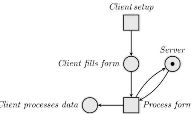
Petri nets are commonly used to express system behaviour. Often, the tokens are understood as threads which execute commands in the program part symbolised by their surrounding place. Thus, transitions model possible control transfer.

Example 1 (Client-server application depicted as a Petri net).

Client fills form

Client setup

Server

Process form Client processes data

Figure 1: Interplay of a server with an arbitrary number of clients

The size of a net N = (P, T, F, M

) is |N | = |P | + |T | + P

p∈P

( P

t∈T

(|F (p, t)| +

|F (t, p)|)) + P

p∈P

M

(p). A transition t is enabled on a marking M if the places from which the transition takes tokens (F(∗, t)) contain at least as many tokens as the transition wants to take. A marking M is called reachable in the net N if there is a sequence of enabled transitions which transforms M

into M .

Petri nets only fulfilling these restrictions are usually called p/t Petri nets to

distinguish them from their bounded subclasses. A net is called k-bounded if no place

in any reachable marking contains more than k tokens. One-bounded nets are called

safe. They have excellent model checking properties: The reachability problem is only

PSPACE-complete for Safe Petri nets while it is already EXSPACE-hard for arbitrary

Petri nets [EN94].

2.2 Mobile Ambients

The Mobile Ambient (MA) calculus focusses on the step-wise transition of processes or devices through administrative domains. These domains are called ambients and their nesting forms a tree structure. Each one possesses a name n. They are entered, left or removed ("opened") by processes via the execution of capabilities π := {in n, out n, open n}.

Definition 1 (Syntax). P is a process term if it is built according to the following rules: P ::= 0 p π.P p n[P ] p !P p νn.P p P|Q p K(~a), where π ={in n, out n, open n}.

A prefix π binds stronger than any other primitive, that is π.P |Q ≡ (π.P )|Q. Next comes the replication !P so that we have !P |Q ≡ (!P)|Q. A restriction is still stronger than the parallel composition: νn.P |Q ≡ (νn.P )|Q. Each ambient’s binding is explicitly stated by its closing bracket since we expect a correct bracket tree.

The ambient symbol n[P ] expresses that P is running within ambient n. Like for the π-calculus 0 has no behaviour, P|Q is the parallel composition of P and Q, K(~a) the call to process identifier K with parameters ~a and νn. P is the restriction which introduces a new name n and limits its scope onto P . A name n occurring in the scope of a νn is called restricted, otherwise called free. The in n and out n capabilities can move an ambient with all its children into or out of a sibling ambient n. The execution of open n removes an ambient n so that its children now belong to n’s former parent.

The transition relation specifies the possible actions giving a formal semantics to the execution of capabilities and calls.

The MA calculus is a classical prefix system so that each action consumes exactly one prefix. Neither restrictions nor ambients are understood as prefixes. Therefore, the transition relation is independent of them.

Definition 2 (Transition relation defining actions). The transition relation defines the four actions:

call: K(~a) K x ~a/~ x y

in: n[in m.P |Q]|m[R] m[n[P |Q]|R]

out: m[n[out m.P|Q]|R] n[P |Q]|m[R]

open: open m.P | m[Q] P | Q

It ignores neighbouring terms completely via P Q ⇒ P | R Q | R and also ignores preceding terms as long as they do not contain prefixes: P Q ⇒ n[P] n[Q], and P Q ⇒ νn.P νn.Q.

All other possible transformations to one MA term are no actions but equivalence

transformations which respect the congruence defined below. They do not influence

the possible actions: P ≡ P

, P Q, Q ≡ Q

⇒ P

Q

. The congruence requires α

conversion of restricted names which we express by the name substitution σ

defined

below. We will see that a term P and its substitution result P σ

(n/l) are congruent

if the substituted name is bound completely in P , that is νn.P ≡ νl.P σ

(n/l).

Definition 3 (Substitution). Let P an MA process term, n a name occurring in P, and l another name. We call a function which replaces each occurrence of n by one of l a substitution. We distinguish the name substitution P σ

(n/l) where l may not occur in P from the parameter substitution P σ

(n/l) without this requirement.

Since process calls allow for the multiple occurrence of a name, we need the second substitution for parameters which doesn’t require the substitute name l to be fresh.

This allows us to write the call action as K(~a) Kσ

(~a/~ x).

Definition 4 (Structural congruence). We define a structural congruence with:

Refl P ≡ P

Symm P ≡ Q ⇒ Q ≡ P

Trans P ≡ Q, Q ≡ R ⇒ P ≡ R

Pers P ≡ Q ⇒ νn.P ≡ νn.Q, P |R ≡ Q|R, n[P ] ≡ n[Q], πn.P ≡ πn.Q Again, as for the π-calculus, | and ν are commutative and associative, with ν also allowing for scope extrusion (νn.(P | Q) ≡ (νn.P ) | Q if n not free in Q). The additional rules are:

νn.m[P ] ≡ m[νn.P ] if n 6= m P|0 ≡ P νn.0 ≡ 0 νn.P ≡ νl.P σ

(n/l) !P ≡ P | !P !0 ≡ 0 0 is understood as equivalent to the empty process (0 ≡ ε).

We define a short notation for MA processes representing the two main components, defining equations and the initial process term. We also enforce that only those equations are defined which are later used, and that the parameter list of each definition is restricted to the finally used parameters.

Definition 5 (MA process). Let D = S

i=1

D

x ~ x

y := P

a set of defining MA equations and I an MA term. The tuple (D, I) is called MA process if

minPara: For all D

all x

∈ ~ x

occur in P

.

closed: All calls to process identifiers in any P

are only done to elements of D.

complete: Each identifier call from the MA calculus term I is only done to elements of D.

reachable: Each D

is either already called in I or in one of the D

callable by I or its (recursive) callees.

In our complexity analysis it will be necessary to reason about the size of such an MA

process. We define it according to the size of π-calculus terms and Safe Petri nets as

the sum over all syntactic elements.

Definition 6 (Size). The size of an MA process (D, I) is size(I) + ( P

i=1

size(D

)) where size(P) for a process term P is defined inductively by

size(0) = 1 size(K(~a)) = 1

size(π.P ) = 1 + size(P) size(n[P ]) = 1 + size(P ) size(!P ) = 1 + size(P) size(νn.P ) = 1 + size(P ) size(P |Q) = size(P ) + size(Q)

and size(D

) for a process equation D

is the size of its right-hand side.

Congruent process terms can have different sizes, for example size(P|0) = size(P ) + 1.

Since we use the process equations in their original form it is important to use the original process’s size for our reasoning rather than some congruent, smaller version.

To simplify matters and exclude pathological cases we restrict ourselves to processes in which restricted names and formal parameters occur only once per equation and are never also used as free names. Analogously to the π-calculus we call this property no clash (NC)[MKH12]. In fact, the original NC criterion was even stricter and forbid multiple restrictions of a name over all equations.

Definition 7 (NC). Let A = (D, I) an MA process with f n(A) all names occurring freely in D or I, rn(A) the set of names occurring restricted in D or I, and pn(A) all names occurring as formal parameters in D. A fulfills the no clash (NC) criterion if

1. The sets f n(A), rn(A), and pn(A) are pairwise disjoint.

2. A name is restricted at most once within an equation D

and in I.

3. A name is used at most once within a formal parameter list.

Together with the restriction to specify only parameters which are later used (Defini- tion 5 on the preceding page) we make sure that each defining equation uses as short a parameter list as possible.

2.3 Bisimulations

Bisimulations link state transition systems which show the same behaviour to an external observer. A bisimulation cares for the action with which a state is transformed into another one. If there are several possible actions in a state, the bisimilar state should be able to perform one action leading into an again bisimilar state for each one of them.

Definition 8 (Act). The set Act of actions consists of all system actions Sys and of the waiting action ε which encodes that the system doesn’t do a step.

Act = Sys ∪ {ε}

The system actions vary with the studied systems but can always be partitioned into modifying actions mod and silent actions τ. The latter are simple prefix removals while the former have some further effect additionally to the prefix removal. For example, the system actions for the MA calculus are all steps according to , i.e.

Sys

= {call, in, out, open} with mod

= {call, in, out, open} and τ

= ∅.

We will concentrate on weak bisimulations where one assumes that the external observer cannot witness silent actions. To abstract them away, we define a relaxed transition relation which allows arbitrarily many silent actions before and after exactly one action α ∈ Act.

Definition 9 (Transition relation with silent actions). Let α ∈ Act. P

⇒

P

iff

∃P

, P

: P

P

P

P

The action α may of course also be a silent action (α ∈ τ ) or even encode no step at all (ε). This new transition relation allows us to define the weak bisimulation:

Definition 10 (Weak bisimulation). A binary relation S ⊆ P × P over processes is a weak bismiulation iff (P, Q) ∈ S implies for all actions α ∈ Act

1. Whenever P

P

, then for some Q

, Q ⇒

Q

and (P

, Q

) ∈ S, 2. Whenever Q

Q

, then for some P

.P ⇒

P

and (P

, Q

) ∈ S.

A process can mimic its bisimilar counterpart’s behaviour. In every state it can do a transition for each action the bisimilar state can process. A weak bisimulation S can be visualised by two commutative simulation diagrams:

P P

Q Q

Q Q

P P

α

S S and

α

S S

αb αb

.

To abstract the concrete relation away and address bisimilarity as a property in general we give the following definition of weak bisimilarity.

Definition 11 (Weak bisimilarity). Two systems T

and T

are called weakly bisimilar (T

' T

) if a weak bisimulation exists between them.

As discussed before the external observer cannot witness silent actions. Thus, a silent

prefix τ does not influence a systems possible actions since it can be consumed before

the required action α without the observer noticing it.

Lemma 1 (Silent actions). Let P an arbitrary process.

P ' τ.P

Proof. The proof can be found in [Mil89, p. 111]. Roughly, τ.P executes τ before mimicking P ’s actual action to establish a simulation of P by τ.P . In the opposite direction τ.P can only execute its silent action which P simply simulates by ε.

In order to combine bisimulations we will make use of their transitivity.

Lemma 2 (Transitivity of weak bisimulations). Let P

, P

, and P

processes and S

⊆ P

× P

and S

⊆ P

× P

weak bisimulations. Then S

◦ S

is also a weak bisimulation.

Proof. The proof can be found in [Mil89, p. 110].

3 Translating MA Processes into Safe Petri Nets – The Idea

The notion already developed by the original "Mobile Ambients"-paper [CG98, p. 144]

that an MA process is a tree gives rise to the idea to use this tree as the data structure for our construction. We depict first MA trees in Section 3.1. Restrictions and ambients are inner nodes and all terms starting with a capability, replication, 0, or a call are leaves. Based on this translation we propose an encoding into Petri net places which are named after all possible parent chid relations. We discuss problematic ambiguities which arise due to the management by name. They are resolved in Section 3.3 where we introduce two distinct name sets A, which keeps the tree unambiguous, and L, which allows us to drop the restrictions. We derive their management via Petri net transitions.

The second key property of the MA calculus is the locality of changes. All capabilities interact with an ambient on an adjacent level so that their influence is also limited to the respective subtree. On one hand this seems only too natural considering the application in firewall modeling and other areas concentrating on step-wise movement, on the other hand it makes a modeling via Petri nets so very natural since – as we will see in Section 3.2 – only few and easily identifiable places are affected by each transition.

3.1 Translating MA Terms into Safe Petri Net Markings

Every MA process term can be represented as a tree where the inner node structure depicts the ambient hierarchy with the restrictions while the leaves are prefix guarded, that is each leaf starts with a capability π, is a call or 0, or a replication. The parallel compositions separate siblings.

Example 2 (Simple ambient hierarchies). The process n[P|m[Q|R]] corresponds to the tree:

n

m R Q

P

.

We do not wish to order a node’s children in the tree but define it to represent all process terms congruent by the rule P |Q ≡ Q|P . Thus, the example tree above also stands for the process terms n[P |m[R|Q]] n[m[Q|R]|P] and n[m[R|Q]|P]. We will later abstract even more congruence rules away so that one marking represents an even larger subset of a process term’s congruence class.

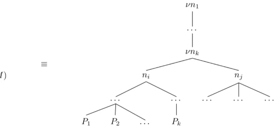
To maintain a tree rather than a forest if parallel compositions occur at the process’s

top level it is necessary to add an artificial root root adopting all so far orphaned

process terms. We will always have this root as to prevent any process term from becom- ing an orphan but only depict it in figures if necessary to keep them representing a tree.

We use the Safe Petri net’s places to represent all possible parent-child relations with the tokens representing the actual ones. E.g., a token on the place labeled n → m shows that an ambient n is a direct child of an ambient m whereas another token on P → m represents a similar relation between a (leaf) process term P and the ambient.

Example 3 (Translating a tree). The process term m[P |n[. . . ]] represents the following tree which is then translated into a net marking:

m n P

⇒

n → m P → m

.

Just like the tree it depicts the marking doesn’t define an ordering on a node’s children.

Thus, each marking represents all processes modulo reordering P |Q ≡ Q|P, too. So far, the parent-child relation is maintained only by name so that problems arise due to ambiguities if there are two ambients with the same name within a process.

Example 4 (Ambiguities in the net). The process term m[P |m[Q]] corresponds to P → m m → m Q → m

. This allows for several interpretations:

m m

Q P

m m P Q

m m Q P

. The last tree is the correct one but the representation allows for all of them.

The ambiguity becomes fatal as soon as capabilities are executed on unintended subtrees leading then to actually unreachable configurations. We will hence later use unique names A = {a

| i = 1, . . . , n} for all ambients. These newly assigned names are not in any relation to the original ones. Thus, we need to make sure that each capability knows "its" ambients.

Even with unique ambient names, yet another problem remains: Identical leaf process terms, so called twins, under one ambient hurt the 1-safeness.

Example 5 (Multiple tokens in the presence of twins). We depict the situation for

the leaf process term P = πn.Q under a:

a

πn.Q πn.Q

⇒

πn.Q → a

. Figure 2: The translation so far allows for multiple tokens

We introduce unique identifiers T = {T

| i = 1, . . . , n}, so called twigs, which we put instead of the leaf below its parent ambient. The relation to the actual leaf term P is maintained via places T

= b P :

a P

⇒

a T

= b P

⇒

T

→ a T

= b P

.

Example 6 (Dealing with twins without and with twigs). With twigs, the situation from Figure 2 translates to

a

T

= b πn.Q T

= b πn.Q

⇒

T

→ a T

= b πn.Q T

→ a T

= b πn.Q

. Figure 3: Representing twigs in the net

Although the introduction of twigs is a rather simple step, we will not incorporate them in our introductory constructions since they create a blow-up on every transition which may hide the central idea behind formalisms. The final construction presented in Section 5.2 will of course provide all features.

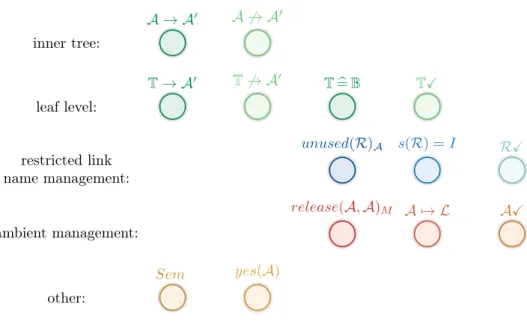
To separate the different groups of places with different functions we will use a color encoding for the rest of this work. The colors are added step-by step and later summarised in Figure 11 on page 37.

3.2 Translating Capability Actions into Petri Net Transitions

The MA calculus is a tree rewriting system since a change in the process state, i.e. the performance of a step according to the transition relation or the congruence ≡, is a transition from one tree into another one.

Example 7 (Tree transition). Let k 6∈ f n(P

). We can then apply the scope extrusion:

n

m R Q

νk P

P

≡

n

m R Q

P

νk

P

. The MA calculus solely provides actions with a local impact. All three capabilities only affect adjacent levels in the tree but behave quite differently on any other account.

Our first rough translation of these actions will visualise which further information we should encode in our net in order to exclude behaviour impossible in MA. We will refine the construction by including twigs and the sophisticated name management.

Restrictions are removed from the tree by the introduction of unique restricted link names R = {r

| i = 1, . . . n}. Even though they are not yet introduced the reader may already assume a restriction-free tree. The call and some other operations are straight forward so that we will only depict them in Section 5.2 when we present the final translation for each MA construct.

We will now shortly summarise the capabilities’ tree transitions. For the rest of this section we fix some naming conventions: Each process incarnation is contained in an ambient

which we call o. It is important to keep in mind that the process variables P , Q, and R used in MA’s transition relation represent arbitrary process terms including those with an ambient or a parallel composition at the top level. However, in the case of open m it will be important to highlight that such a process can be a parallel composition. We will do so by using Q

to Q

instead of Q.

3.2.1 The Capability Action in m

The action n[in m.P |Q]|m[R] m[n[P |Q]|R] corresponds to:

o

m R n

Q in m.P

o m

R n

Q P

. Figure 4: o[n[in m.P |Q]|m[R]] o[m[n[P |Q]|R]]

We make the parent n of in m.P a child of its former sibling m. We neither depict Q nor R nor any further children of o in our net fragment since they do not interfere with the transition. In order to avoid n jumping through the tree we need to verify that they are siblings: We assumed that o is n’s parent and thus need to check that it is also m’s parent via a test on m → o.

2Remember that at leastrootis such an ambient.

n → m

m → o

n → o

in m.P P → n

in m.P → n

We depend on in m.P , o, and n for the transition. Thus, there is one such transition per (o, n, in m.P )-combination.

3.2.2 The Capability Action out m

The action m[n[out m.P |Q]|R] n[P |Q]|m[R] corresponds to:

o m

R n

Q out m.P

o

m R n

Q P

.

Figure 5: o[m[n[out m.P|Q]|R]] o[n[P|Q]|m[R]]

The operation out m is inverse to in m. The ambient n, formerly the parent of out m.P and the child of ambient m, becomes m’s sibling during the transition.

Therefore, the transition has to know m’s parent (which we assume to be o) to introduce n as its new child. This requires the test on m → o here.

n → m

m → o

n → o

out m.P P → n

out m.P → n

In comparison to an in transition, the n → m place is a token source while n →

o now receives a token. Everything else is equal for both transitions (of course,

now we consume the out m prefix) and thus we again need one transition for each (o, n, out m.P )-combination.

3.2.3 The Capability Action open m

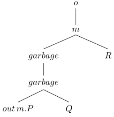
The action open m.P | m[Q] P | Q corresponds to:

o

m

Q

Q

Q

open m.P

o

Q

Q

Q

P

. Figure 6: o[open m.P | m[Q]] o[P | Q]

The ambient m is removed by its sibling open m.P . This requires all processes which were so far m’s children to introduce themselves to m’s and open m.P ’s common parent o. Obviously, a new test on o is required but it can be realised with the change from open m.P → o to P → o which is anyway necessary.

Unfortunately, the Safe Petri net’s structure so far is not able to decide when all subprocesses of m subscribed to o. We install complement places to overcome this short-coming. Now we may either inspect all place and complement place pairs in a predefined order or we can visit them concurrently. Since the latter approach requires an additional huge transition to unite the intermediate visits into an "all-ambients- considered" place – and since additional arguments will be necessary when arguing for the transitions’ correctness – we will implement the first approach. Depending on the Petri net model checker at hand one may of course choose the concurrent approach instead.

m → o

m 6→ o

open m.P P → o

open m.P 6→ o

P 6→ o release(m, o)

Sem

open m.P → o

We use the semaphore to block other transitions which may influence the actual tree.

This will prevent undesired races before we are able to restore a correct tree. After

the actual open m.P transition the tree is already degenerated into a forest since the

connection m → o is erased. At first the second tree with root m possesses the children Q

to Q

but during the chain’s execution these children vanish. It doesn’t make a difference wether an ambient or a leaf process is m’s child so that we unite them in a set M = {P | P leaf term} ∪ {n | n name} \ {m, o} which we stepwisely process.

release((M

→ m) o) M

→ m M

6→ o M

→ o

M

6→ m test((M

6→ m) o)

release(m, o)

release(m, o)

The chain is hard-coded via progress logging places release(m, o)

where release(m, o)

is consumed for the (∗ + 1)-th transition and release(m, o)

is fed by it. We can unify the depicted first steps with all intermediate steps by a slight mod- ification: Rather than release(m, o) the open transition should fill release(m, o)

.

The process chain provides the same two transition for each ambient or leaf process term M

under m. In the case of a token on the complement place, nothing has to be done and the token is simply passed to the logger for the next step. However, if the token is on any place M → m we have to remove this connection and replace it by M → o before allowing the next transition to take over. The last transition re-installs the semaphore:

release((M

→ m) o) M

→ m M

6→ o M

→ o

M

6→ m test((M

6→ m) o)

release(m, o)

Sem

. Finally, we are done and can be happy that only two ambients were involved. In fact, the release-chain only depends on the (m, o)-combination while the original open-transition depends on the (o, open m.P )-combination.

3.2.4 The Semaphore’s Necessity

The semaphore blocks all transitions interfering with the actual tree no matter wether

they affect the inner ambient tree or the leaf level. We illustrate inconsistencies

appearing if we did not use it on the example of out m:

Example 8 (Possible race without semaphore). We consider the transition for o[m[n[out m.P |Q]|R]] o[n[P|Q]|m[R]] if a release(o, o

) sequence is processed in parallel, that is we formerly had o

[open o.S|l[m[n[out m.P|Q]|R]]]. The processing of nothing but the open transition without its subsequent release chain has yield:

o

o m

R n

Q out m.P open o.S

open

o

S

6 o m

R n

Q out m.P

. The ambient o should now vanish and all its children (here only m) should move under

o

. If we now assume that the release chain starts its execution and the ambient n is tested before out is fired, but m is not, the token on n 6→ o is seen and allows the test chain to proceed. Now out fires, thus n is hung under o. The release step on m correctly puts m below o

but the already tested n remains:

o

S

6 o n X

Q P m R

release((m→o)o⁰)

o

m R S

6 o n X

Q P

. Since the n to o relation was already considered it won’t be tested again so that n remains under the actually removed o and we run into an inconsistent system state.

The new second root o should actually have vanished and n should be another child of o

. Instead, n’s connection to the main tree is lost.

The strict use of the semaphore prevents such unpleasant behaviour. We now turn our attention to guaranteeing the uniqueness of names.

3.3 Managing Names in the Petri Net

As we pointed out in Example 4 on page 16 the relation by name causes ambiguous

trees since several ambients may carry the same name. We now use the ambient name

set A which our Petri net will use instead of the original name. In order to react to

the right capabilities the connection to that name is still maintained. We remove the

restrictions from the tree by assigning a unique name from the new set of restricted

link names R. Their management requires new commands which we incorporate in

the MA process equations via a preprocessing. We derive transitions to manage both

link and ambient names.

Names and their respective positions store the information in the MA processes.

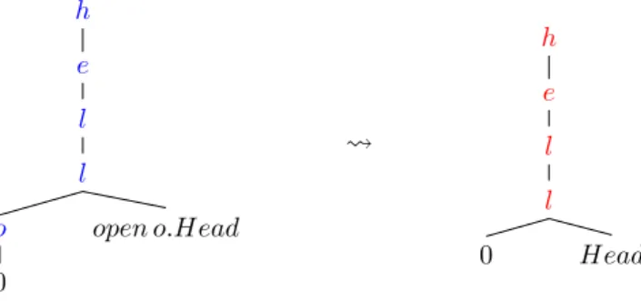
The proof of Turing-completeness for the MA calculus [CG98, p. 149f] encodes the tape into a chain of nested ambients. The ambient’s name corresponds to the current symbol on the dedicated tape position.

Example 9 (Ambient hierarchy encoding a word).

h e l l

open o.Head o

0

h e l l

Head 0

Figure 7: "hello" becomes "hell"

Hence, the saving of name and position information in each ambient is the heart of the information storage in the MA calculus. Capability operations and the addition of new ambients via ambient spawning (n[P ]) manipulate such information.

3.3.1 Distinguishing Link from Ambient Names

Actually, a name m accomplishes two completely different tasks: It stores information in the ambient tree (m[. . . ]) via its name and position but it also maintains the connection between the ambients called m and the capability operations (in m, out m and open m).

We want to separate these concerns in our construction. Hence, we distinguish link names (L), which maintain the connection between capabilities and the actual instance in the tree, and the globally unique instance names which we call ambient names (A) and which form the tree. We demand A ∩ L = ∅.

root

m

Q

m

Q

open m.P

Figure 8: Link name m and ambient name m

Link names L unify all ambients in a scope and represent them in capabilities and

process calls. We will enforce link names to be unique, too, so that we can manage

their relation to the ambients (a 7→ l) by name and remove the restrictions from the

tree. The incorporated ambients of one link name should not be affected by any other link name, nor should any ambient without a corresponding link name exist. Hence, the link names will induce a partition of the ambients into scopes.

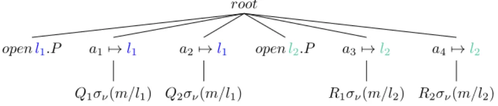
Example 10 (A capability’s scope). In the process νm.(open m.P | m[Q

] | m[Q

])

| νm.(open m.P | m[R

] | m[R

]) each open m-capability may only affect the two m- ambients in its restriction’s scope. We assign the link names l

and l

:

root

a

7→ l

R

σ

(m/l

) a

7→ l

R

σ

(m/l

) open l

.P

a

7→ l

Q

σ

(m/l

) a

7→ l

Q

σ

(m/l

) open l

.P

Figure 9: Different scopes replaced by different names

The omission of restrictions keeps the tree flat. Because of NC only locally restricted names may carry the same name. This makes a distinction between public link names P and restricted link names R appropriate. We have L = P ∪ R.

In summary, link and ambient names are globally unique but link names may occur several times within a process incarnation. They are only present at the leaf level, while the ambient names only occur above this level in the inner tree and at most once there.

3.3.2 Assigning a Restricted Link Name r ∈R

We assign a new restricted link name whenever we process a leaf νn.P : The net non-deterministically chooses a currently unused name r ∈ R and substitutes n by r in the whole term P . Since n’s scope can only be intermitted by a new νn which is not allowed within the same process equation due to NC we can substitute n by r on the whole leaf (νn.P P σ

(n/r)). It is absolutely desirable to rename the n-ambients as well: this propagates the information on which name r to link. Our substitution also replaces occurrences in process calls and thus makes sure that the name is passed on to subsequent equations.

νn. P νn. P 6→ a

νn. P → a

P σ

(n/r) 6→ a

P σ

(n/r) → a

r X Sem

The token on r X guarantees that r is currently unused. The transition occupies the name and performs νn.P P σ

(n/r). The inner ambient hierarchy is not touched.

3.3.3 Assigning an Ambient Name

When processing an ambient spawn l[P ] we choose an arbitrary unused name a

∈ A (a

X ) and replace the link name l ∈ L by a

, while not changing P at all. Note that this is no substitution on P but just a very local renaming in one position. We store the knowledge that a

reacts to l-capabilities on the place a

7→ l.

a

→ a

a

6→ a

a

X a

7→ l

r[P]

P → a

P 6→ a

l[P ] 6→ a

l[P ] → a

Sem

This transition is more complex than the link version since it must also integrate a

into the ambient tree.

3.3.4 Releasing an Ambient Name

An ambient hierarchy remains even if there is no process running in it any more. This makes the release of an ambient name fairly easy, since the only situation to do so is when processing an open capability. There are only minor changes necessary to adapt the open procedure presented in Section 3.2.3 on page 20. We now use the name l and write open l to indicate that we work on a link name.

a

→ a

a

6→ a

a

7→ l

open l.P

a

X

P → a

open l.P 6→ a

open l.P → a

P 6→ a

release(a

, a

)

Sem

Due to the separation of link and ambient names we now need to check via a place a

7→ l that a

reacts on l capabilities, namely on open l. We mark a

as unused via a

X and erase a

from the ambient hierarchy by the release(a

, a

) procedure. This procedure remains unchanged in comparison to 3.2.3 on page 21 and is hence not repeated here.

3.3.5 Releasing a Restricted Link Name

The releasing of a restricted link name is only possible if it is completely unused in the process incarnation P . In the marking representing this incarnation it should neither appear in a leaf process term nor have any ambient linked to it. A marking with a name r which is unused but not marked as unused (r X ) corresponds to an MA process term νr.P where r does not occur in P . In this analogy our release performs the congruence transformation to P .

We must start by verifying that the name is forgotten among all leaves since a leaf carrying a spawn could easily introduce a new link while an open command could remove one: As long as there are leaves using a name r the information on its use in the tree is volatile.

Forgotten Among All Leaves? – Maintaining a Name’s Spread

Wether or not a name is forgotten at the leaf level can best be monitored via the name’s spread among the Petri net leaves. A name r’s spread s(r) is the number of Petri net leaves which currently use it. Although the spread’s behaviour is totally dynamic the positions at which this value changes are already visible in the process equations. Thus, we can do a preprocessing on the original process equations with the original names n. We mark the relevant positions with the commands used(n) and unused(n), respectively. These new commands allow the net to log the appropriate changes to a name’s spread. They are executed during runtime and thus performed on the instance name r. As soon as a spread declines to 0 we immediately know that the respective name is forgotten among all leaves (r X

). The one-safeness requires us to use one place s(r) = i per possible spread value i. Whenever we process a restriction νn.P we initialise the spread of the chosen name r with 1.

νn. P νn. P 6→ a

νn. P → a

P σ

(n/r) 6→ a

P σ

(n/r) → a

r X Sem

s(r) = 1

The substitution P σ

(n/r) and subsequent calls also instantiate the corresponding

used and unused commands with r.

Each used(r) action increases r’s current spread s(r) = i by 1:

used(r) P → a

P 6→ a

used(r).P 6→ a

Sem

s(r) = i + 1

s(r) = i used(r).P → a

.

The unused(r) action behaves similarly, but reduces the spread by moving the token from s(r) = i onto s(r) = i − 1. In every case but the lowest option with s(r) = 1 we simply have:

unused(r) P → a

P 6→ a

unused(r).P 6→ a

Sem

s(r) = i − 1

s(r) = i unused(r).P → a

. If r’s spread is s(r) = 1 before the unused(r) execution, the name is now forgotten among all leaves. Instead of s(r) = 1 we remove the count completely and mark r X

. We will now discuss where to put the used and unused commands.

Incorporating the Necessary Information – the Preprocessing

We determine the relevant positions by examining the right-hand side of each defining equation as well as the initial term. Commands can be set for a name r freshly restricted in this term as well as for a formal parameter x inherited from some former process term. The latter may cause problems if the name instantiating x is public.

We can easily deal with these problems by an additional transition for each public name p ∈ P which simply consumes the command:

(un)used(p)

P → a

P 6→ a

(un)used(p).P → a

(un)used(p).P 6→ a

.

Another way to address this problem is to exclude public names from parameter lists.

We will discuss this in Section 7.2 on page 66.

At first, only the leaf which carried the restriction νn can know the name n and thus later the chosen instance. Since there is no name passing mechanism like there is in the π calculus the leaf cannot spread its knowledge to other leaves arbitrarily.

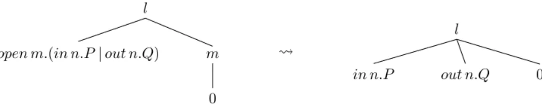
The name’s spread can only increase if the leaf splits itself into two leaves. This can either happen due to a parallel composition or due to a replication. If after a parallel composition P|Q both leaves use the name n we should increase s(n) by 1.

Example 11 (Spread increase with parallel compositions). Both process terms follow- ing the parallel composition use n so that its spread increases as soon as this parallel composition is no longer prefixed.

l

m 0 open m.(in n.P | out n.Q)

l

0 out n.Q

in n.P

Figure 10: Counting leaves using n: n’s spread changes from 1 to 2

We can check for each parallel composition P |Q in each defining equation (and in I) whether P and Q both continue to use a name n which was used before the parallel composition. If they do, we put the command used(n) before the parallel composition.

One could argue that this increases the spread too early, before the parallel composition is actually processed, but since we are only interested in the question wether the spread is above 0 or not this can cause no harm.

However, if we put the used(n) command say in front of Q we could reach wrong conclusions: Imagine s(n) = 1, that is the leaf carrying P|Q is the only leaf knowing n. If we now freed P for execution it could easily reach and execute its unused(n) out of which the net would conclude s(n) = 0 although Q still knows n but did not tell the net yet.

The dealing with the replication !P is similar to that for the parallel composition: we must put a used command right behind the replication sign ! for each name occurring in P . But since a name occurring in a replication term can never become unused our spread count is useless there. We only keep it to exclude the wrong conclusion of a spread of 0 which may otherwise arise just like it may in the parallel composition’s case.

The unused commands are put behind each last occurrence of a name on the right-hand side of a process equation. Due to minP ara in Definition 5 on page 11 this last occurrence is always either a capability or a spawn. Thus, we check behind each capability πn and spawn n[Q] wether n is used in the following process term Q.

If it is not used we put the unused(n) command before Q.

Forgotten in the Ambient Tree

As soon as the instance r is forgotten among all leaves we also need to make sure that no ambient is linked onto r. Here the static relationship between an ambient and its link name plays an important role: During an ambient’s whole life time it is bound to one link name. Only by opening it becomes free again and can then be assigned to a new link name l during a spawn. However, we know that this new name isn’t our name r since r is forgotten among all leaves and therefore cannot exist in a spawn.

Thus, we only have to implement a simple test chain where we protocol for each ambient name a ∈ A that it is not linked to r. As we discussed before it does not matter when we test the ambients as long as the name r is forgotten among all leaves.

This makes the consuming of the semaphore unnecessary for the whole procedure which we again implement sequentially.

Each of the chain’s transitions takes a place unused(r)

as input

. This place encodes that all ambients up to a

have already been inspected and none of them was linked onto r. The ambient a

is next. The possible situations are:

• a

7→ r: If a

is linked onto r we may not proceed but are trapped. Since no r capabilities exist any more this ambient and its link to r will never be removed.

Thus, r will never become unused.

• a

7→ l

6= r: If a

is linked onto a name different to r we can immediately proceed to a

.

• a

X : The ambient name a

is currently unused. It cannot become linked to r since no spawn on r exists. Thus, we can immediately proceed to a

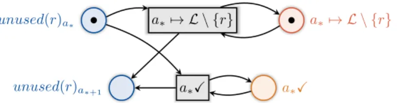
. The corresponding transition set is:

a

7→ l

a

7→ r

a

X unused(r)

unused(r)

a

7→ l

a

X .

The transition for the link name l

stands subsidiarily for all L \ {r} transitions. We reflect the blocking by no transition in the case that a

is linked onto r. If the chain passes all ambients successfully the last transition marks the name r as unused (r X ).

3To avoid the distinction between the chain’s first and intermediate transitions, we markunused(r)a₁

instead ofrXleaves inunused(r).

3.4 Guaranteeing Finiteness

So far, we were not worried about the finiteness of the Petri net. With our design decision to maintain the tree by using distinct identifiers for each ambient and twig we are forced to limit their respective numbers. We introduce a breadth bound b which gives a bound for T and an additional bound d to limit the overall number of ambients and thus A. A bound for R can be constructed out of them.

Definition 12 (b, d-bounded process). An MA process term is called b, d-bounded if its number of ambients is at most d and the overall number of parallel compositions is at most b − 1, that is there are at most b leaf processes. An MA process is called b, d-bounded if each reachable congruence class contains at least one b, d-bounded instance.

Conceptually, the bound d is a depth bound for the ambient tree and thus for the process since it constraints the nesting depth of ambients. A depth bound on MA processes was also necessary in [RVMS12] where they derived decidability of coverability by a translation into ν-MSR. This logic incorporates a restriction ν which makes it convenient for the translation but hard for the checking – only a non- primitive recursive coverability checking procedure exists and reachability is in general undecidable. However, the restriction operator allows them to enforce uniqueness by different scopes rather than different names so that their result is independent of any breadth bound. It is unknown wether pure MA reachability is decidable if we only require a depth bound. But since it is known to be undecidable for MA’s ancestor π ([MG09, p. 15]) where depth is the number of names a "leaf" process knows we expect it to require high complexity if at all possible for MA. Our breadth restriction allows for an only PSPACE-complete decidability procedure which is as low as one can usually get in verification.

The breadth and depth bounds are in general not computable since this would allow us to decide how much space a Turing machine uses. Recall that MA can simulate arbitrary Turing machines (Argument in Section 3.3 on page 23 subsuming the proof in [CG98, p. 149f]). Rather than restricting the process to be b, d-bounded we could therefore set artificial bounds to generate a finite net. Even if the process itself was unbounded it might possess interesting runs – e.g. counter-examples – which respect the artificial bounds. Section 7.4 will provide the necessary extensions and a small example. The reader who finds it more convenient may already check that all translation schemes in principle extend to unbounded processes, too. Only the simulation may block if we require more names or twigs than we have: We can process a parallel composition or a replication only if a new twig is available for the new leaf.

This requires a management of unused twigs T

via places T

X which is similar to the ambient name management.

MA Parameters

Apart from the breadth and depth bound there are some size parameters which depend on the respective MA process (D, I) where each D

∈ D has a parameter vector ~ x

. We call the maximal number of parameters in a defining equation κ = max

(|~ x

|).

We have the number of public names p and the number of process equations d

= |D|.

The maximal number c of restrictions a leaf process term may spawn is crucial for the possible calls: Only public, freshly restricted names and passed restricted names are possible parameters. We must compare all possible threads through each process equation in order to determine c. Since a parallel composition splits one leaf into two we have to consider both resulting subprocess terms in combination with the part before the split. Thus, we multiply out each parallel composition: A.(P|Q) is transformed to A.P and A.Q. Of course, the results are not equivalent to the process term before since instead of one shared name we now receive two independent names n for each restriction νn in the prefix A. If we apply the transformation to each process equation including I we receive a number of threads T h

with i = 1, . . . , m. The maximal number c of new restrictions is simply the maximal number of restrictions in one of these threads c = max(#ν (T h

) | i = 1, . . . , m).

It is obvious that all of the process parameters are bound by the process’s size n.

4 From MA to rMA

The introduction of the used and unused commands exceeds the MA calculus’s means.

We therefore define the refined MA calculus, shortly called rMA calculus, which is capable of expressing the additional commands. We recapitulate and analyse the preprocessing algorithm which bridges the gap between the two formalisms. The proof that rMA introduces no new behaviour is done by establishing a bisimulation. It is our first step towards a bisimulation between MA and our Petri nets.

4.1 Preprocessing

The first step towards rMA is the preprocessing algorithm for the introduction of used and unused commands to a process P = (D, I). We consider the initial term I as the right-hand side of a parameterless equation D

∈ D so that we then simply deal with all defining equations. The set rn(D

) consists of those names which are freshly restricted in D

.

We need a predicate occur(n, P ) which tests syntactically wether the name n occurs in the term P . It can be implemented linearly in length(P ) which is always in O(length(D

)). The actual algorithm pre(P ) is performed independently for each D

∈ D by the following replacement:

f o r each πn.P :

i f not occur(n, P ) then s e t πn.unused(n).P f o r each n[P] :

i f not occur(n, P ) then s e t n[unused(n).P]

f o r each P|Q :

f o r each n ∈ ~ x

∪ rn(D

) :

i f occur(n, P ) and occur(n, Q) then s e t used(n).(P|Q) f o r each !P :

f o r each n ∈ ~ x

∪ rn(D

) :

i f occur(n, P ) then s e t used(n).P

Since the name addressed by the capability and the spawn is unique we can set at most one unused command behind each one of them. On the contrary, it may be necessary to put several used commands before a parallel composition or a replication – one for each name which is spread to P and Q or used in P .

The algorithm can be implemented by one pass through the process term which

determines the respective positions to be checked. Of course, neither the number

of capabilities and spawns nor of parallel compositions and replications may exceed

length(D

). The check behind a capability and spawn only requires one execution

of occur while each parallel composition may require up to |~ x

∪ rn(D

)| · 2 many

executions which is twice as much as the replication requires. Although dominating

the capabilities’ and spawns’ time demand those are still in O(length(D

)). Thus,

even in the worst case where the equation mostly consists of parallel compositions we

are still in O(length(D

))

for its analysis. This guarantees that our preprocessing for

all equations may be performed in O(n

) for n = size(P ).

4.2 The Refined MA Calculus

Since rMA is a rather simple extension of MA we will only give new definitions where necessary and otherwise expect the given MA definition to extend to rMA as well.

Definition 13 (Syntax). P is an rMA process term if it is built according to the following rules: P ::= 0 p π.P p n[P ] p τ.P p !P p νn.P p P |Q p K(~a), where π = {in n, out n, open n} and τ = {used(n), unused(n)} for a name n.

This is essentially the same definition as Definition 1 on page 10, only the new commands are added. We give τ n the same binding priority as πn, otherwise adopting the priorities given for the MA calculus. Additionally, we need to adapt the transition relation in order to deal with the new actions.

Definition 14 (Transition relation for rMA). The rMA transition relation is that of the MA calculus with the additional rules:

use: used(n).P P unuse: unused(n).P P

Thus, the new commands are simple silent actions where the prefix is consumed but no modification on the tree is necessary. They play no role in rMA’s semantics and do not influence the system behaviour. However, we know that the Petri net will take a quite different view on them.

We adapt the structural congruence given in Definition 4 on page 11 accordingly by the addition of P ≡ Q ⇒ τ.P ≡ τ.Q with τ = {used(n), unused(n)} and add the rule size(used(n).P ) = size(unused(P )) = 1 + size(P) in Definition 6 on page 12.

4.3 Bisimulation between MA and rMA

MA and rMA calculus enjoy the prototype of weak bismiulation since their only difference lies in the silent actions which rMA has while MA doesn’t have them. As already implied by Lemma 1 on page 14 any process term derived out of a term P by adding silent actions to P is bisimilar to it.

Lemma 3. Let P an MA process. The relation '

= (P, pre(P )) linking an MA process and the rMA process derived by preprocessing it is a bisimulation.

Proof. The rMA process pre(P ) is an enrichment of P by silent used and unused actions. No reordering or replacement of the MA process’s actions happens. Thus, we can establish a bisimulation between the two processes by Lemma 1 on page 14.

We can define a b, d-bounded rMA process in analogy to Definition 12 on page 30.

Since we will establish a Petri net translation only for b, d-bounded MA processes it is desirable to know that the bisimulation '

between MA and rMA processes retains the bounds.

Lemma 4. Let P a b, d-bounded MA process. The rMA process pre(P ) is also

b, d-bounded.