EMTLAB: A Toolbox for the Analysis of Electromagnetic Tracking Data in Brachytherapy Goetz ThI

Advances in Applied Science Research, 2017, 8(4):40-61

ISSN : 0976-8610 CODEN (USA): AASRFC

INTRODUCTION

Breast cancer is the most frequent cause of female mortality in Europe. Radiation therapy is often one of the few drastic means to fight this disease. High Dose Rate Brachytherapy (HDR-BT) marks a recent major progress in radiation therapy [1]. After surgical excision of the tumorous tissue often a radiation treatment follows where the tumor bed is irradiated with high energy radiation [2,3] stemming from highly active radioactive compounds like ¹⁹²Ir. Because of the high energy dose (30-50) [Gy] deposited in the tissue by these radioisotopes, a precise determination of the locations, where the radiation source has to be placed, is essential. To place the radiation source as close as possible

EMTLAB: A Toolbox for the Analysis of Electromagnetic Tracking Data in Brachytherapy

Goetz ThI^1,2*, Herzberger F¹, Tome AM³, Hensel B² and Lang EW¹

1CIML, Biophysics, University of Regensburg, 93040 Regensburg, Germany

2Center for Medical Physics and Engineering, University of Erlangen-Nürnberg, 91052 Erlangen, Germany

3IEETA, DETI, Universidade de Aveiro, 3810-193 Aveiro, Portugal

ABSTRACT

Background: High dose rate brachytherapy (HDR-BT) of female breast cancer patients relies on electromagnetic tracking (EMT) for localizing the prescribed dwell positions of the radiation source. A collection of machine learning techniques like Particle Filtering (PF), Singular Spectrum Analysis (SSA), Ensemble and Multivariate Empirical Mode Decomposition (EEMD/MEMD) represent powerful signal processing techniques and are employed in this study to achieve this goal. Information-theoretic similarity measures allow comparing extracted signal components for artifact identification and elimination.

New toolbox: We present a new toolbox, called EMTLAB, which is designed as an extensible toolbox for electromagnetic tracking data analysis. It contains all machine learning techniques mentioned above and is written in MATLAB^®. Results: EMTLAB offers the practitioner a convenient way to easily and efficiently perform particle filtering, signal decomposition and manual or automatic artifact removal with an SSA, an EEMD or MEMD in combination with three similarity measures: Pearson correlation, Jensen-Shannon divergence or Kull back-Leibler divergence. As demonstrated with illustrative examples, EMTLAB offers a complete and almost fully automatic signal processing chain for an analysis of EMT data sets collected during a HDR-BT. In addition, EMTLAB represents a user-friendly graphical user interface (GUI), which also provides convenient means to visualize the results in illustrative graphs. A number of screen shots helps in understanding the functioning of the signal processing chain and the use of the GUI.

Conclusion: EMTLAB is a reliable, efficient and automated solution for processing and analyzing EMT sensor data from a HDR-BT, while employing different physical models of system dynamics. This sensor tracking by particle filtering allows to adapt the analysis to different dynamical models and the SSA and EMD algorithms provide an easy means to remove from the data artifacts stemming from breathing modes or measurement device malfunctioning.

Keywords: Electromagnetic tracking, Particle filtering, Empirical mode decomposition, Singular spectrum analysis, Similarity measure

to the tumor bed, a number of catheters is implanted into the female breast by a surgical intervention. The position of the catheters with respect to the anatomy is verified by an X-ray computed tomography (CT) image, where a medical physicist tracks by hand the shape of the catheters and inputs this information into a treatment plan. The latter defines so-called dwell positions and dwell times for the later radiation treatment [4,5]. The treatment usually extends over several days with, usually, short treatment sessions one or two times a day. Between these sessions the patients can move around freely which might cause some small catheter displacements. The latter may also be caused by tissue swelling (edemata) as a consequence of the surgical intervention. Hence, before any treatment session, the validity of the existing treatment plan needs to be controlled by test measurements of the dwell positions with a sensor, which is moved inside the catheters to the prescribed dwell positions. The sensor position is determined by an electromagnetic tracking device, which encompasses a magnetic field generator (FG) and a remote after loader. The former generates an inhomogeneous magnetic field and the latter moves the solenoid sensor inside the catheters in accord with the treatment plan. A precise determination of the sensor positions during these test measurements is hampered by the breathing activity of the patients. Even worse, patients often speak during the measurements, rendering their breathing motions rather irregular. In addition, due to patient movements between the sessions, catheter displacements may occur. Because of the high energy dose deposited by the radiation, it is tantamount to follow the treatment plan as closely as possible. This constraint seems unrealistic in clinical practice.

In a recent study, Goetz et al. [6] pursued the possibility to reconstruct catheter shapes and concomitant sensor dwell positions from electromagnetic tracking (EMT) measurements alone without recourse to an external reference such as fiducial sensors. This EMT only protocol avoids additional errors which might be introduced by external referencing.

Because of frequent re-positioning of the field generator (FG), multi-dimensional scaling (MDS) [7-9] had to be employed to estimate an optimal common coordinate system for comparison of the different measurements [6]. The latter, however, are inevitably fraught with measurement noise. In a subsequent study, Goetz et al. [10,11] thus proposed applying several machine learning techniques like particle filters (PF) [12,13], empirical mode decomposition (EMD) [14-17] and singular spectrum analysis (SSA) [18-20] accompanied by information-theoretic similarity measures [21], to achieve an artifact-free and noise reduced sensor signal, which best reflects the true sensor dwell positions, hence catheter shapes. It was shown that any dwell position deviations from the treatment plan can be quantified, and possible error sources identified early enough to be corrected or for the treatment plan to be adapted. In critical cases treatment can even be stopped on the basis of the particle filter tracking.

The current study designs a toolbox which implements all these techniques. It thus provides convenient means for any potential user to apply such data analysis techniques to EMT signals recorded during test measurements. The latter need to be performed before any radiation treatment within an HDR-BT. The signal processing chain implemented in this toolbox starts with a particle filtering of the raw sensor signal. The latter is inevitably ballasted with measurement noise, hence any tracking device observes noise-contaminated dwell positions while, after particle filtering, the underlying system states are obtained. To apply a particle filter, a state evolution model needs to be designed from prior knowledge about the dynamical system under consideration. As an additional complication, the observed sensor states also contain contributions from breathing activities. The latter can be removed by applying empirical mode decomposition to the sensor signal. Both an ensemble EMD and a multivariate EMD are implemented. Often also high amplitude artifacts, resulting from device malfunctions, appear in the recorded signals. They can be suppressed by applying an SSA to the recorded signals. Both signal decomposition techniques, EMD and SSA, achieve artifact-free sensor signal tracks by omitting during reconstruction those signal components which can be assigned to the artifacts.

The assignment task is achieved via information-theoretic similarity measures like Pearson or Spearman correlation, Kullback-Leiber divergence and Jensen-Shannon divergence, all of which are implemented in the toolbox as well.

EMTLAB TOOLBOX

EMTLAB is an interactive MATLAB toolbox for processing EMT data. It provides a graphical user interface (GUI) which enables users to flexibly and interactively process their data and tuning their parameters. EMTLAB provides plenty of methods for importing, visualizing, preprocessing data and remove artifacts. Using EMTLAB, users can apply advanced signal processing techniques to their data such as:

• Particle filter tracking (PF)

• Artifact removal (automatically or manually)

• Visualizing their results

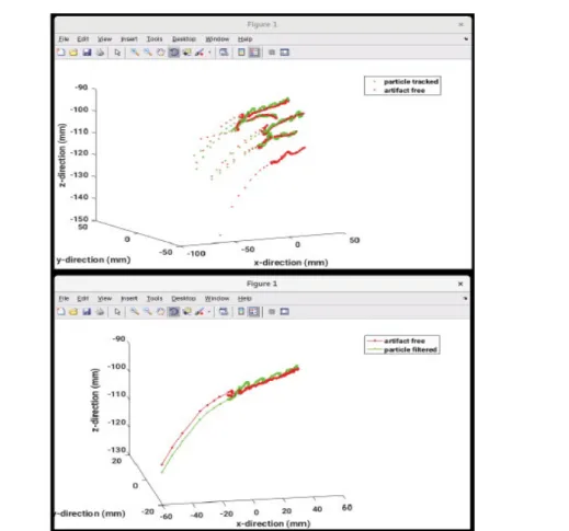
In Figure 1, the basic concept of the EMTLAB toolbox is illustrated. One can start with the raw EMT data which consist of:

• Electromagnetic tracking (EMT) data from a 5 DoF sensor,

• Coordinates reflecting basic knowledge about the observed sensor trajectory (BK) and

• Electromagnetic tracking data from the 6 DoF fiducial sensors (FID), which monitor breathing artifacts.

These data represent noise-contaminated versions z t^{( )}≡ ztof the underlying states of the system x0:twhich are unobservable thus unknown. The goal is to estimate the sequence x0:tof these system states from the time-dependent observations. Such an estimate can be achieved by applying the particle filter toolbox to the data to obtain a denoised EMT signal. The results are saved in a data structure called 'PF'. The tracked data still contains artifacts like the breathing and movement artifacts as well as artifacts due to a malfunctioning of the measuring device. Several signal decomposition techniques like singular spectrum analysis (SSA) and ensemble or multivariate empirical mode decomposition (EEMD (MEMD)) are implemented. Employing similarity measures like Spearman correlation (SP), the Jensen-Shannon divergence (JS) and the Kullback-Leibler divergence (KL) help to identify artifact-related signal components which then can be removed automatically, or manually, by neglecting their contribution to the signal reconstruction from its components. Different strategies are followed:

• Large amplitude artifacts often correspond to the principal component obtained via SSA. They can be suppressed by subtracting them during the reconstruction process.

• Artifacts with characteristic periods can be identified by comparing them to intrinsic modes resulting from an EEMD decomposition. A good example represent breathing modes in EMT recordings, which form one of the characteristic intrinisc modes and are similar to the fiducial sensor signals, hence can be identified via any of the similarity measures implemented, either automatically or manually (HH).

The results are saved according to the used artifact removal method (AR_*).

METHODS

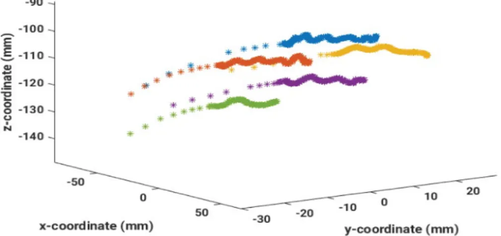
Electromagnetic tracking (EMT) is an appealing method for measuring solenoid sensor movements in magnetic fields without the need of an external reference signal. A typical example is the dwell position tracking of solenoid sensors inside catheters during an HDR-BT. Hence, the algorithms are illustrated with EMT sensor data measuring a superposition of the sensor movement along a catheter implanted in a female breast and a breathing motion during an HDR-BT treatment (Figure 2). These signals can be analyzed favorably with the EMTLAB, especially as they are generally non-linear and non-stationary.

Figure 1: Flowchart of the EMTLAB toolbox

Three steps which have to be performed, namely signal denoising by applying PF, artifact removal by applying EEMD/MEMD and SSA, and comparing components employing similarity measures.

PARTICLE FILTER

The toolbox realizes sensor tracking via a sequential Monte Carlo sampling technique [22,23], called Particle Filter, which approximates the posterior density by a weighted sum of particles (set of random samples) according to

1 1 .)

( ( )x t_k+ ≡x etc_k+

( )

1 1: 1| 1 1

1

( _k | _k) ^N _{k k}ⁱ _{k k}ⁱ

i

p x ₊ z w ₊

δ

=

≈

∑

Where, w_{k k}ⁱ+_1| represents the weight of particle i 1

xk+ . Based on the weights and the samples, relevant statistics can be estimated. For a very large number of samples the particle filter approaches an optimal Bayesian estimate of the posterior probability density.

A solution for this state estimation problem is Bayesian filtering by iteratively computing the posterior density

( |_{k l k}: )

p x z . In the toolbox, the latent state of the sensor x_k at discrete time t^kcan be estimated by knowing the history of observations z_{l k:} = z_l,…, z_k at timest₁, ,… t_k. For the posterior distribution of the latent state variables (filtering density), one obtains by marginalizing the Chapman-Kolmogorow equation the following relation

1: 1: 1

( |_{k k}) ( | ) ( |_{k k k k} ) p x z ∝ p z x p x z −

Where, p x z( |_{k 1: 1k−}) represents the model prior and p z x( | )_{k k} the data likelihood.

The state evolution model is based on a physical model of the dynamical system f x( ,_k _k^{( )x} ). The measurements z_1:k

can be represented by an observation model h x( , )_k _k^m , where _k^m represents the measurement noise and



Figure 2: Example data where five catheters were measured by an EMT sensor. A superposition of the movement along the catheter and a breathing motion is clearly visible.

THE MODEL EQUATIONS

As input for the particle filter, a state evolution model as well as an observation model is needed. The dynamical variables of the system can be collected in a state vector x t( )∈^N, which describes the dynamic state of the system.

The state evolution model f(...) describes the dynamic evolution of the system.

(

)

1 , ^x ( 1| 0: , 1: ) ( 1| )

k k k k k k k k

x ₊ = f x  p x ₊ x z = p x ₊ x (1)

Where, ^{( )x} ∈^N denotes the state noise and k=1,2,... denotes discrete time instancesx_k. The sequence of state vectors x_k is assumed independent of the sequence of observations z_1:k and forms a Markov process [25].

In the toolbox, the state evolution model implements the spatial dependence of the dynamic state via a polynomial function, and its time dependence by a Fourier series. The EMTLAB was originally constructed for tracking sensor movement along a catheter which is inserted into a female breast. The physical model of this situation is a superposition of the movement along the catheter, represented by a polynomial function, and the breathing motion, which is approximated by a Fourier expansion. The user can choose whether he wants to consider a superposition of both functions, and only one of them.

If the spatial dependence should be modeled by a polynomial function, prior knowledge of the observed sensor trajectory needs to be available in form of coordinatesr_i =( , , )x y z_{i i i} . From this set of 3D coordinates, a static trajectory

f l

( )

l

3

11 12 13 14 2

1 21 22 23 24

31 32 33 34

( )

1

k T k k

k

a a a a l

f l a a a a l A L

a a a a l

    

   

=       ⋅ = ⋅

Where, A∈ ³× ^4and l^k∈. The order of the polynomial function can be chosen between 1 and 5 by the user.

The length of the sensor movement l_k is computed as, 0 1 k

k i

i

l l δ

=

= +∑ ^{, where} 1 if sensor is moved along the trajectory c

0 if sensor is stopped at a dwell position

i

mm δ = ^ mm

 (2)

For each distance, the evolution model f1_CT( )l_k provides the corresponding ( , , )x y z coordinates of the sensor along the trajectory. Figure 3 exemplifies how a fit to a polynomial function can be achieved from known dwell positions from the treatment plan. This results in a model for the corresponding sensor trajectory.

With HDR-BT applications, it is regularly the case that the trajectory of the sensor is known in a coordinate system differing from the treatment plan system. For this reason, the evolution model f l1T( )k needs to be transformed to the coordinate system of interest. To estimate this transformation, we take the first measured EMT sensor position, because its distance from the endpoint of the catheter is known precisely. This location can be estimated in the EMT coordinate system and then enters the state evolution model [10]. A shift vector s and a rotation matrix Rcomplete the transformation according to:

x′ = ⋅ +R x s (3) Consequently, the state evolution model f l₁( )_k can be expressed in EMT-coordinates as:

1( )_k 1_T( )_k

f l = ⋅R f l +s (4)

Hence, the trajectory f l₁( )_k now refers to the EMT-coordinate system. The coordinate transformation is updated after each tenth iteration, and after removing the artifacts of the measured signal by applying an EEMD and using the Pearson correlation to identify the artifacts. In Figure 4, the coordinate transformation is calculated exemplarily for a late time point where already many system states have been estimated.

However, the state estimation model also depends on time. To account for any superimposed breathing motion, or other time-dependent distortion, the sensor motion needs to be modeled by a Fourier series, yielding:

1 2

1 2

0 0

1

( , ) ( ) ( )

( ) ( )

/ 2 ( ( ) ( ))

k k f

CT k f

m

k k f

k

f l t f l f t R f l s f t

R A L s a b cos k t c sin k tω ω

=

= + +

= ⋅ + + +

= ⋅ ⋅ + + +

∑







(5)

Where, a b c, ,_{k k}∈^3and m is the order of the Fourier series, which can be chosen by the user between 0 and 10.

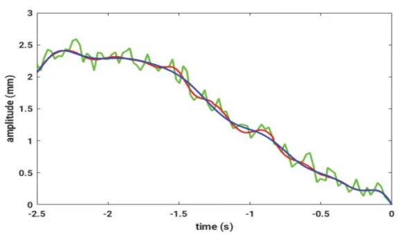
For this model, the positional data, received from the fiducial sensors, is used. First, noise reduction of the signal is achieved by applying an EEMD. Afterwards, a Fourier series is fit to the data. In Figure 5, these steps are shown for measured EMT data, where a breathing motion is superimposed.

The observation vector zcollects all observations at

t

Figure 3: Known treatment plan dwell positions (red stars) of the sensor trajectory and a polynomial t of oder 3 (blue line)

Figure 4: One catheter, where the points correspond to the information from the treatment plan, are transformed to the particle filtered blue points, which result after removing the breathing artifact

(

)

1 1 1

1 0: 1

1 0:( 1) 1: 1 1

,

( | ) ( | )

( | , ) ( | )

k k km

k k k k

k k k k k

z h x

p z x p z x

p z x z p z x

+ + +

+ +

+ + + +

=

=

=



(6)

Where, ^m∈^N denotes the measurement noise. Assuming, that the probability of an observation forms a Markov process with respect to the history of the state vectorx_k, then any observation h depends on the current state only.

The various noise distributions p(^{( )x}) and p(^{( )m} ) are also assumed to be mutually independent and known.

For the observation model h , the simplest possible choice is implemented, corresponding to a normally distributed measurement noise. This finally yields:

( , , , , )

k k

k h

k k

l x h l x y z t y z t

  

  

= +

  

  



THE SAMPLING-IMPORTANCE-RESAMPLING SCHEME

The filtering densityp x( _k+1|z_{1:( 1)k+} ), can be approximated by a weighted set of particles{ , }x w0:ⁱk k i^{i N}=1. The particle filter (PF) updates the Bayesian recursion relations at each iteration by generating and evaluating N different trajectories according to:

(

)

(

)

p x z − =w − − p x x−

Where, the weights correspond tow_{k k}ⁱ| = p x

(

)

Figure 5: A breathing signal for one spatial direction measured by fiducial sensors (green), the denoised signal (red) and the Fourier series (blue)

probabilities is computed with the state evolution model. By importance sampling from the likelihood of the observationsp z x

(

)

( ) ^{( )}

1:( ) 1

( |_{k k} ) _k | _kⁱ , _{k k} | _k

p x z ≈ p x x ₋ z ∝ p z x (7) The following weighted update, based on the state evolution model, results if samples are drawn from the likelihood

( )

| 1| 1 | 1

i i i i

k k k k k k

w = w_{− −} p x x ₋ (8) Finally, the weights {w_{k k i}ⁱ_| }^N₌₁ are normalized to sum to one.

The importance sampling from the likelihood becomes unstable with increasing N. It can be stabilized by resampling [27,28]. By multiplying particles with an importance weight and eliminating particles with low weights, a new set of N particles can be draw. Finally, the following approximate distribution is obtained [29].

(

)

1

ˆ _k, _k ^{N i} ( _k ⁱ_k)

i

p x z n x x

Nδ

=

=

∑

Where, x_0:ⁱ_k is the number of copies of particle trajectoryx_0:ⁱ_k. In the toolbox, re-sampling is performed for each time step.

The toolbox offers the following three re-sampling schemes, from which the user can choose:

• multinomial resampling

• systematic resampling

• residual resampling

These resampling schemes are based on a multinomial selection of N particles with replacement from the original particle set { }x^{i N}_i=1[10,30].

To sum up, particle filtering is realized employing the Sampling Importance Resampling (SIR) algorithm [31]. The re-sampling is applied at every iteration and the state transition probability p x

(

)

By looking at the system evolution from t_{k-1} to t_k, the following steps can be applied [13]:

Step 1: For ^{i= …1, ,N}new particles xⁱk from the importance density can be draw by employing the transition model

( )

1 1

1

( )_k ^{N i}_{k k}| _kⁱ

i

q x w p x x− −

=

=

∑

To do so, choose particle i r= and choose a random number

r

(

)

Calculate corresponding weights by using the corresponding likelihood

(

)

i i

k k k

w = p z x

The samples x_kⁱ are taken from p x z( _k | 1: 1_k− ) and re-weighting them accounts for the evidence of the observations

zk.

Step 2: Calculate the total weight

1

N i

k k

i

W w

=

=

∑

and normalize the particle weights

1 1,....,

i i

k k k

w W w= ⁻ ∀ =i N

Step 3: Re-sample the particles by doing the following:

Compute the cumulative sum of weights W_kⁱ=W_kⁱ−₁+wⁱ_k;∀ = …i 1, , ,N W⁰ =0 Let i=1 and draw a starting point u₁from a uniform distribution U(0,N⁻¹) For ^{j= …1, ,N} do the following

• move along the cumulative sum of weights by setting u_j = +u N₁ ⁻¹( 1)j−

• while u_j >W set i iⁱ = +1

• assign samples x_k^j = xⁱ_k

• assign weights w_k^j =N⁻¹

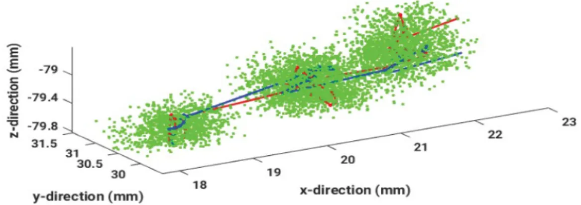
Having many degenerate particles with very small weights can be avoided by this resampling procedure. If the resulting samples contain many redundant particles, it can lead to a loss of diversity. This sample impoverishment is often observed in case of small process noise. In Figure 6, showing 200 estimated particles per data point, the resulting sensor trajectory and the measured points are illustrated for example data.

SINGULAR SPECTRUM ANALYSIS

Depending on the EMT measurement system, the tracked particle trajectory can still contain large amplitude artifacts (outliers) and time dependent mode contributions, i.e., breathing motion. Through a singular spectrum analysis (SSA) [18,32], the recorded non-stationary time series can be decomposed, and artifacts can be removed from the EMT recordings during signal reconstruction. Thus, if the EMT of the sensor movement contains a breathing mode superimposed on its motion inside the catheter, an independent measure of the artifact-related motion component can be obtained by 6 DoF fiducial sensors fixed to the chest of the patient. This contaminating breathing signal can be decomposed also within the toolbox by applying an SSA. For further processing, usually only the dominant principal component needs to be retained.

The well-known signal analysis technique, Singular Spectrum Analysis (SSA), decomposes the original time series into a sum of orthogonal components. These components can be interpreted as trends, oscillatory components or structureless white noise [18-20].

Figure 6: Estimated particles (green), EMT-measured points (blue) and the resulting trajectory (red) are compared in a three dimensional plot

Let x t( )=(x t( )₁x t( )_T )^T≡ x_T=(x₁x_T)^T be a sensor signal with zero mean and a total length T. We can obtain by ( , , ( 1))^T

k k k L

x = x … x+ − selecting an embedding dimension K and a proper segment length L T ^{such that}

1

T K L= + − . The analysis of a time series with SSA can be done in two steps [20,33]:

A decomposition step, which encompasses embedding of the time series into Kdelayed coordinates combined with an eigendecomposition of a correlation matrix, and

A reconstruction step, which encompasses reverting the embedding and anti-diagonal averaging.

Especially the latter step reconstitutes an ^{(L K× )} - dimensional trajectory matrix [33], from which the reconstructed time series can be obtained by reverting the initial concatenation step. The trajectory matrix then reads

[ ]

1 2 3

2 3 4 1

3 4 5 2

1

1 2 1

K K K K

L L L L K

x x x x

x x x x

x x x x

X x x

x x x x

+ +

+ + + −

 

 

 

 

= =  

 

 

 

 

 





 

   

   



(10)

Where, the columns of this Hankel matrix are formed by the time series segment of length L T≤ and its delayed versions. An alternative representation yielding trajectory matrices with a Toeplitz structure would also be possible [20]. A K K× - Dimensional, real-valued and symmetric matrix can be obtained by considering the matrix dot product X X^T . This matrix possess an eigendecomposition.

(

)

{ ,λ_k k= …1, , }K . The projection of the data onto them yields proper features according to

k k

z = Xv (12)

Now signal denoising can be achieved by neglecting components during reconstruction with eigenvalues smaller than a certain threshold. The latter must be low enough to indicate that the related variance reflects noise contributions.

This, however, implies that the reconstructed trajectory matrix doesn't have the structure of a Hankel matrix anymore.

By anti-diagonal averaging of the latter an approximation to the original time series is obtained.

In summary, by applying an SSA to the recorded EMT solenoid sensor signals, large amplitude artifacts can be removed by deleting the principal mode related with the largest eigenvalue which typically reflects such large amplitude artifacts.

ENSEMBLE EMPIRICAL MODE DECOMPOSITION

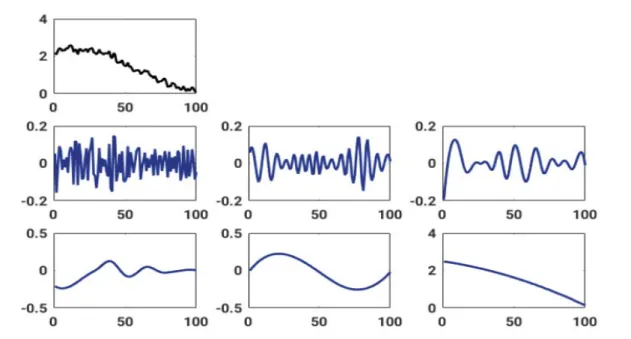
After the raw EMT sensor signal is noise-reduced and particle filtered, the sensor signal still contains artifacts. More precisely, because the recorded EMT sensor signals contain several motion components, i.e., the sensor movement inside a catheter and the overlaid breathing motions, the toolbox offers a signal decomposition employing either an EEMD or an MEMD. An EEMD can be used to identify those modes which contain information about the artifact- related contributions similar to the independently measured fiducial sensor signals. In Figure 7, the decomposition of a fiducial signal into its intrinsic modes is shown.

Figure 7: The top row represents the original breathing signal as measured by the ducial sensors. The following two rows contain the intrinsic modes, which result from applying an EEMD and which are ordered from top left to bottom right with increasing period

Any non-stationary and non-linear time series can be decomposed by an EEMD [14,15,34] into a list of oscillatory components with characteristic time scales ordered with increasing period. A signal is decomposed in a sum of intrinsic modes (IMFs) with zero-mean amplitude- and frequency-modulated components.

One can express the original signal x t( )as:

( )

{ } { ( ) }

( ) ( )

( ) ( ) ( ) ^j ( ) ( )lim ( ) ( ) ( )^j ( )exp ( ) ( )exp ^t ( )

n n j n n n n j j j j

x t x t t c t r t x t x t c t Re a t i tφ Re a t i ω t dt

−∞

→∞ ′ ′

= +^ =

∑

∫

Where, ( )_n t denotes random noise contributions, c_n^{( )j} =c^{( )j} +_n( )t represents the intrinsic mode obtained for the n^th noise observation, ( )x t is the true signal and ( )r tn the remaining non-oscillating trend. By averaging all the c^{( )j of}

the ensemble the resultant IMF c^{( )j} is obtained. The related instantaneous frequency is denoted by ^{ωj[rad s/ ]=d tφ}_dt^{j( )}, the time-dependent amplitude by a t_j( ) and φ_j( )t =

∫

MULTIVARIATE EMPIRICAL MODE DECOMPOSITION

The plain EMD can be extended to a Multivariate Empirical Mode Decomposition MEMD [17,38]. Plain EMD can only decompose one-dimensional time courses. MEMD can be interpreted as a multivariate approach by taking the response of a system from several channels as a signal in an n-dimensional space. This multivariate signal is tried to be decomposed into IMFs, which can no longer be seen as oscillatory modes rather should be considered rotational modes. To solve the problem of no proper definition of extrema in n dimensions, the aspect of creating envelopes around the time course is generalized to n dimensions [17]. To sample the n-dimensional space as uniformly as possible, a set of Hammersly-sequenced n-dimensional direction vectors is introduced. To extract the extrema of one-dimensional representations of the signal, it is projected onto each direction vector. Afterwards the signal is re-projected into the n-dimensional space, resulting in sets of n-dimensional minima and maxima for each one- dimensional projection. With these optima, n-dimensional envelopes can be constructed. From now on, the procedure and the stopping criterion are as in a plain EMD. The only differences concern the comparison of the number of zero

crossings and the number of extrema. Zero crossings in n-dimensional space are not properly defined. An advantage of the MEMD compared to its univariate counterpart is that frequency scales of corresponding IMFs align [17].

Also a noise assisted (NA-MEMD) or an ensemble noise assisted (ENA-MEMD) variant is proposed for MEMD [39,40]. The NA-EMD introduces, in addition to the signal channels spanning the n-dimensional space of the multivariate signal, a number l of noise channels carrying white Gaussian noise with noise amplitude of 2-10% of the signal amplitude [40]. After EMD is performed, the l noise channels are discarded. The principle of several realizations of IMFs by using different random initializations of noise contributions to several NA-MEMD runs resembles the same principle as used within an EEMD in the univariate case and is called ENA-MEMD.

After particle tracking and denoising the raw EMT signal, artifacts can be removed by applying the EEMD or MEMD to the sensor signal and also to the fiducial signal overlapping the moving sensor signal. After decomposing both signal the intrinsic mode which best represents the fiducial signal can be identified. Tracked EMT signal reconstruction while omitting the contribution from the intrinsic fiducial mode yields an uncontaminated sensor signal. The decomposition has to be repeated, depending on the signal to remove all the artifacts. The choice of IMF can be drawn by human or automatically with the aid of similarity measures.

SIMILARITY MEASURES

The EMT system measures a superposition of the sensor motion inside the catheter and the periodic motions of the sensor as a consequence of breathing. The latter contribution can be independently measured with fiducial sensors fixed to the chest of the patient. Separating both motions can be achieved by sensor signal decomposition with an EEMD or an MEMD [10]. To identify those intrinsic modes, which most closely resemble the breathing mode contribution, similarity measures are used. The selected contaminating intrinsic modes will be neglected during signal reconstruction. The user can choose between several alternative measures of similarity offered by the toolbox.

To measure point-wise, linear correlations between stochastic, normally distributed variables, the most frequently used measure is the Pearson correlation coefficient [41]. Let x=(x₁x_L)^{T and y=(y1yL)T} be two time series segments with size L T≤ represented as L-dimensional vectors. The Pearson correlation coefficient c is calculated as follows

1 1 1

2 2

2 2

1 1 1 1

, ) (

L L L

l l l l

l l l

L L L L

l l l l

l l l l

L x y x y

c x y

L x x L y y

= = =

= = = =

  

−   

  

=

   

−  − 

   

∑ ∑ ∑

∑ ∑ ∑ ∑

(14)

However, Pearson correlation fails if the data sets also contain nonlinear correlations. In such cases, entropy- based similarity measures might be more appropriate. The Shannon entropy H X( ) [42,43] and its related mutual information I X Y( , ) as well as several divergences [44] are based on distances between distributions of the variables.

The following similarity measures are available in the toolbox:

The Kullback-Leibler divergence (KLD) [45] or relative Entropy measure a non-symmetric similarity between two distributions P and Q

1

ˆ ˆ ( )

( ) ( ( ) ( )) ( )ln ( )ˆ

L l

KL KL l

l l

D X Y D p x q y p x p x

q y

=

 

≡ =  

 

∑

 

Where, the stochastic variables are normalized according to:

1 1

ˆ_{l L} ^l and ˆ_{l L} ^l

l l

l l

y x

y x

y x

= =

= =

∑ ∑

If p x( ) is modeled by means of q y( ), information is lost. Considering the relation of mutual information ^{I X Y( , )} to relative entropyDKL, we obtain for two stochastic variables X and Y the following expression

( )

, 1

( , ) ( ( ), ( )) ( , ) ( ) ( ) ( , )ln

( ) ( )

L l l

KL l l

l l l l

p x y I p x p y D p x y p x p y p x y

p x p y

′ ′

′= ′

 

= =  

 

∑



The Jensen-Shannon divergence (JSD) [46,47] is a smoothed and symmetrized version of the KLD. The square root of the Jensen-Shannon divergence is a metric often referred to as Jensen-Shannon distancedJS= JSD.

Let p x q y^{( ), ( )}be two realizations of discrete probability distributions P,Q. The ^{JSD P Q(}  ⁾ then is defined as:

( )

1 1

1 1 1 1

( ) ( ) ( )

2 2 2 2

N N

KL KL n n n n

n n

JSD P Q D P P Q D Q P Q H w P w H P

= =

 

   

=  + +  + = ∑ −∑

   (16)

Where, w w1= 2=1/ 2and for the second equality N = 2, P P Q P≡ 1, ≡ 2, is used. Thus, the JSD measures the similarity of each of the two considered distributions to their corresponding mixture distribution.

A comparison of the results of different similarity measures contained in the toolbox and the judgment of a human observer considering deviations between EMT data collected during a Breast Brachytherapy is discussed by Goetz [11].

RESULTS

The basic functionality of the EMTLAB toolbox is to provide a proper data processing chain for analyzing EMT data with PF, SSA, EMD and MEMD. Thus, the toolbox includes a group of MATLAB functions for applying PF, SSA [48,49], EEMD [15], MEMD [17] and the similarity measures PC, JS and KL.

The EMTLAB menu includes three main parts:

• The first part is used to set parameters and settings for the particle filtering. Afterwards, the single channel or multi-channel results can be visualized conveniently.

• The second part contains various methods to automatically remove artifacts from the particle filtered signal and, again, visualize the results.

• The third part offers the possibility to manually remove artifacts by the user through an interactive interface.

DATA STRUCTURE

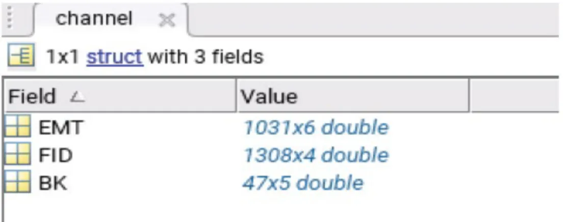
The data processed by the toolbox has to have an array structure to be used in MATLAB. For each EMT measured channel, three fields exists: the measured raw data points saved as EMT, the raw fiducial signals saved as FID and, finally, the dwell positions from the treatment plan, considered as basic knowledge and saved as BK. Therefore the input data are represented by a 6×M structure, where n is the number of measured channels. In Figure 8, the workspace in MATLAB is exemplified for some the test data. The structure is extended after particle filtering (PF) and after artifact removal (AR). The whole structure is saved in the input folder with the filenames extended with 'PF' or 'AR'.

The EMT measurements are saved as a 6×M matrix where M is the number of measured points (Figure 9). The six dimensions contain the following information:

1. dim.: time from start of the measurement in seconds 2. dim.: x-values according to the measurement defined origin 3. dim.: y-values according to the measurement defined origin 4. dim.: z-values according to the measurement defined origin 5. dim.: length how far the sensor was moved away from start 6. dim.: information of the status of the sensor ('stop', 'in' or 'out')

The second input matrix in the structure is denoted FID, where the four dimensions are identical to the first four dimensions of the EMT matrix. The BK matrix has a dimension 3×P where P is the number of known dwell positions from the treatment plan, and the three dimensions reflect the spatial coordinates of the data points in an arbitrary coordinate system.

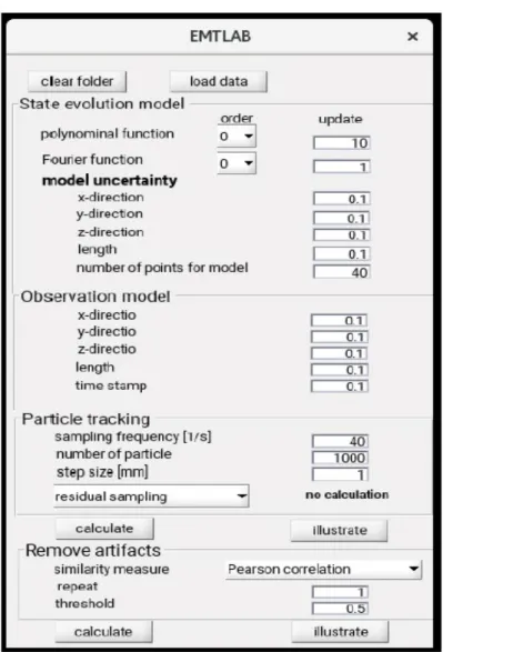
RUN PARTICLE FILTERING AND VISUALIZE RESULTS Figure 10 presents the main window of the EMTLAB toolbox. It contains the following topics:

State evolution model

The first part is used to perform the particle filtering. In the top box, named 'State evolution model', the user can set the order of the polynomial function as well as of the Fourier series to model the system dynamics. Furthermore, the number of measured points is fixed, after which the coordinate transformation of the time-dependent model should be updated. If the order is set to zero, either the temporal or the spatial model is set to be constant. To specify the uncertainty of the model, the standard deviation for each spatial direction, for the length of the sensor movement and for the time stamps can be inserted by the user also. Finally, the first measured position needs to be modeled to be able to estimate particles. Therefore, the number of FID data has to be larger than the EMT data, and for a certain number of points their spatial locations have to be specified for use in the first model estimates.

Figure 8: Screen shot of the MATLAB workspace of the 5 3 structure of the test data

Figure 9: Screen shot from the MATLAB workspace of the 6M matrix of the EMT test data

Observation model

In the second box, named 'Observation model', the following quantities can be set by the user: the standard deviation in each spatial direction, the total length of the sensor trajectory, measured from the starting point and the time stamp of the dwell positions. With these parameters, the accuracy of the measured data can be individually specified.

Particle tracking

In a third box, named 'Particle tracking', the sampling frequency of the EMT system, the number of particles and the distance between two possible sensor 'stop'-positions can be set. Moreover, the user can choose between the following three resampling schemes in a pop up menu:

• Systematic resampling

• Residual resampling

• Multinomial resampling

By pushing the button 'calculate', particle filtering is applied in parallel to the spatio-temporal sensor data of all channels, i.e., catheters, while the toolbox freezes its state. These calculations need some time, obviously; hence, intermediate results are stored in an output folder. The latter is in the same folder as the toolbox. After particle filtering the sensor EMT data from all catheters, the initial MATLAB structure becomes extended with the PF matrix and is saved in the Input folder under a filename with the extension .pf (Figure 11).

Figure 10: The EMTLAB main user interface. This window is used for particle filtering. Through this window, users can choose the data, model settings and appropriate parameters for the filtering