The empirical mode decomposition and the Hilbert spectrum for nonlinear and
non-stationary time series analysis
B y Norden E. Huang1, Zheng Shen2, Steven R. Long3, Manli C. W u4, Hsing H. Shih5, Quanan Zheng6, Na i-Chyuan Y e n7,
Chi Chao Tung8 a n d Henry H. Liu9
1Laboratory for Hydrospheric Processes/Oceans and Ice Branch, NASA Goddard Space Flight Center, Greenbelt, MD 20771, USA
2Department of Earth and Planetary Sciences, The John Hopkins University, Baltimore, MD 21218, USA
3Laboratory for Hydrospheric Processes/Observational Science Branch, NASA Wallops Flight Facility, Wallops Island, VA 23337, USA
4Laboratory for Atmospheres, NASA Goddard Space Flight Center, Greenbelt, MD 20771, USA
5NOAA National Ocean Service, Silver Spring, MD 20910, USA
6College of Marine Studies, University of Delaware, DE 19716, USA
7Naval Research Laboratory, Washington, DC, 20375-5000, USA
8Department of Civil Engineering, North Carolina State University, Raleigh, NC 27695-7908, USA
9Naval Surface Warfare Center, Carderock Division, Bethesda, MD 20084-5000, USA
Received 3 June 1996; accepted 4 November 1996
Contents
page
1. Introduction 904
2. Review of non-stationary data processing methods 907
(a) The spectrogram 907
(b) The wavelet analysis 907
(c) The Wigner–Ville distribution 908
(d) Evolutionary spectrum 909
(e) The empirical orthogonal function expansion (EOF) 909
(f) Other miscellaneous methods 910
3. Instantaneous frequency 911
4. Intrinsic mode functions 915
5. The empirical mode decomposition method: the sifting process 917
6. Completeness and orthogonality 923
7. The Hilbert spectrum 928
8. Validation and calibration of the Hilbert spectrum 933
9. Applications 948
(a) Numerical results from classic nonlinear systems 949 (b) Observational data from laboratory and field experiments 962
Proc. R. Soc. Lond.A (1998)454, 903–995 c 1998 The Royal Society
Printed in Great Britain 903 TEX Paper
10. Discussion 987
11. Conclusions 991
References 993
A new method for analysing nonlinear and non-stationary data has been devel- oped. The key part of the method is the ‘empirical mode decomposition’ method with which any complicated data set can be decomposed into a finite and often small number of ‘intrinsic mode functions’ that admit well-behaved Hilbert trans- forms. This decomposition method is adaptive, and, therefore, highly efficient. Since the decomposition is based on the local characteristic time scale of the data, it is applicable to nonlinear and non-stationary processes. With the Hilbert transform, the ‘instrinic mode functions’ yield instantaneous frequencies as functions of time that give sharp identifications of imbedded structures. The final presentation of the results is an energy–frequency–time distribution, designated as the Hilbert spectrum.
In this method, the main conceptual innovations are the introduction of ‘intrinsic mode functions’ based on local properties of the signal, which makes the instanta- neous frequency meaningful; and the introduction of the instantaneous frequencies for complicated data sets, which eliminate the need for spurious harmonics to rep- resent nonlinear and non-stationary signals. Examples from the numerical results of the classical nonlinear equation systems and data representing natural phenomena are given to demonstrate the power of this new method. Classical nonlinear system data are especially interesting, for they serve to illustrate the roles played by the nonlinear and non-stationary effects in the energy–frequency–time distribution.
Keywords: non-stationary time series; nonlinear differential equations;
frequency–time spectrum; Hilbert spectral analysis; intrinsic time scale;
empirical mode decomposition
1. Introduction
Data analysis is a necessary part in pure research and practical applications. Imper- fect as some data might be, they represent the reality sensed by us; consequently, data analysis serves two purposes: to determine the parameters needed to construct the necessary model, and to confirm the model we constructed to represent the phe- nomenon. Unfortunately, the data, whether from physical measurements or numerical modelling, most likely will have one or more of the following problems: (a) the total data span is too short; (b) the data are non-stationary; and (c) the data represent nonlinear processes. Although each of the above problems can be real by itself, the first two are related, for a data section shorter than the longest time scale of a sta- tionary process can appear to be non-stationary. Facing such data, we have limited options to use in the analysis.
Historically, Fourier spectral analysis has provided a general method for examin- ing the global energy–frequency distributions. As a result, the term ‘spectrum’ has become almost synonymous with the Fourier transform of the data. Partially because of its prowess and partially because of its simplicity, Fourier analysis has dominated the data analysis efforts since soon after its introduction, and has been applied to all kinds of data. Although the Fourier transform is valid under extremely general conditions (see, for example, Titchmarsh 1948), there are some crucial restrictions of
the Fourier spectral analysis: the system must be linear; and the data must be strict- ly periodic or stationary; otherwise, the resulting spectrum will make little physical sense.
The stationarity requirement is not particular to the Fourier spectral analysis;
it is a general one for most of the available data analysis methods. Therefore, it behoves us to review the definitions of stationarity here. According to the traditional definition, a time series,X(t), is stationary in the wide sense, if, for allt,
E(|X(t)2|)<∞, E(X(t)) =m,
C(X(t1), X(t2)) =C(X(t1+τ), X(t2+τ)) =C(t1−t2),
(1.1)
in whichE(·) is the expected value defined as the ensemble average of the quantity, and C(·) is the covariance function. Stationarity in the wide sense is also known as weak stationarity, covariance stationarity or second-order stationarity (see, for example, Brockwell & Davis 1991). A time series,X(t), is strictly stationary, if the joint distribution of
[X(t1), X(t2), . . . , X(tn)] and [X(t1+τ), X(t2+τ), . . . , X(tn+τ)] (1.2) are the same for allti and τ. Thus, a strictly stationary process with finite second moments is also weakly stationary, but the inverse is not true. Both definitions are rigorous but idealized. Other less rigorous definitions for stationarity have also been used; for example, piecewise stationarity is for any random variable that is stationary within a limited time span, and asymptotically stationary is for any random variable that is stationary whenτ in equations (1.1) or (1.2) approaches infinity. In practice, we can only have data for finite time spans; therefore, even to check these defini- tions, we have to make approximations. Few of the data sets, from either natural phenomena or artificial sources, can satisfy these definitions. It may be argued that the difficulty of invoking stationarity as well as ergodicity is not on principle but on practicality: we just cannot have enough data to cover all possible points in the phase plane; therefore, most of the cases facing us are transient in nature. This is the reality; we are forced to face it.
Other than stationarity, Fourier spectral analysis also requires linearity. Although many natural phenomena can be approximated by linear systems, they also have the tendency to be nonlinear whenever their variations become finite in amplitude.
Compounding these complications is the imperfection of our probes or numerical schemes; the interactions of the imperfect probes even with a perfect linear system can make the final data nonlinear. For the above reasons, the available data are usu- ally of finite duration, non-stationary and from systems that are frequently nonlinear, either intrinsically or through interactions with the imperfect probes or numerical schemes. Under these conditions, Fourier spectral analysis is of limited use. For lack of alternatives, however, Fourier spectral analysis is still used to process such data.
The uncritical use of Fourier spectral analysis and the insouciant adoption of the stationary and linear assumptions may give misleading results; some of those are described as follows.
First, the Fourier spectrum defines uniform harmonic components globally; there- fore, it needs many additional harmonic components to simulate non-stationary data that are non-uniform globally. As a result, it spreads the energy over a wide frequen- cy range. For example, using a delta function to represent a flash of light will give
a phase-locked wide white Fourier spectrum. Here, many Fourier components are added to simulate the non-stationary nature of the data in the time domain, but their existence diverts energy to a much wider frequency domain. Constrained by the energy conservation, these spurious harmonics and the wide frequency spectrum cannot faithfully represent the true energy density in the frequency space. More seri- ously, the Fourier representation also requires the existence of negative light intensity so that the components can cancel out one another to give the final delta function.
Thus, the Fourier components might make mathematical sense, but do not really make physical sense at all. Although no physical process can be represented exactly by a delta function, some data such as the near-field strong earthquake records are of extremely short durations lasting only a few seconds to tens of seconds at most.
Such records almost approach a delta function, and they always give artificially wide Fourier spectra.
Second, Fourier spectral analysis uses linear superposition of trigonometric func- tions; therefore, it needs additional harmonic components to simulate the deformed wave-profiles. Such deformations, as will be shown later, are the direct consequence of nonlinear effects. Whenever the form of the data deviates from a pure sine or cosine function, the Fourier spectrum will contain harmonics. As explained above, both non-stationarity and nonlinearity can induce spurious harmonic components that cause energy spreading. The consequence is the misleading energy–frequency distribution for nonlinear and non-stationary data.
In this paper, we will present a new data analysis method based on the empirical mode decomposition (EMD) method, which will generate a collection of intrinsic mode functions (IMF). The decomposition is based on the direct extraction of the energy associated with various intrinsic time scales, the most important parameters of the system. Expressed in IMFs, they have well-behaved Hilbert transforms, from which the instantaneous frequencies can be calculated. Thus, we can localize any event on the time as well as the frequency axis. The decomposition can also be viewed as an expansion of the data in terms of the IMFs. Then, these IMFs, based on and derived from the data, can serve as the basis of that expansion which can be linear or nonlinear as dictated by the data, and it is complete and almost orthogonal. Most important of all, it is adaptive. As will be shown later in more detail, locality and adaptivity are the necessary conditions for the basis for expanding nonlinear and non-stationary time series; orthogonality is not a necessary criterion for our basis selection for a nonlinear system. The principle of this basis construction is based on the physical time scales that characterize the oscillations of the phenomena. The local energy and the instantaneous frequency derived from the IMFs through the Hilbert transform can give us a full energy–frequency–time distribution of the data.
Such a representation is designated as the Hilbert spectrum; it would be ideal for nonlinear and non-stationary data analysis.
We have obtained good results and new insights by applying the combination of the EMD and Hilbert spectral analysis methods to various data: from the numerical results of the classical nonlinear equation systems to data representing natural phe- nomena. The classical nonlinear systems serve to illustrate the roles played by the nonlinear effects in the energy–frequency–time distribution. With the low degrees of freedom, they can train our eyes for more complicated cases. Some limitations of this method will also be discussed and the conclusions presented. Before introducing the new method, we will first review the present available data analysis methods for non-stationary processes.
2. Review of non-stationary data processing methods
We will first give a brief survey of the methods available for processing non- stationary data. Since most of the methods still depend on Fourier analysis, they are limited to linear systems only. Of the few methods available, the adoption of any method is almost strictly determined according to the special field in which the application is made. The available methods are reviewed as follows.
(a) The spectrogram
The spectrogram is the most basic method, which is nothing but a limited time window-width Fourier spectral analysis. By successively sliding the window along the time axis, one can get a time–frequency distribution. Since it relies on the tradition- al Fourier spectral analysis, one has to assume the data to be piecewise stationary.
This assumption is not always justified in non-stationary data. Even if the data are piecewise stationary how can we guarantee that the window size adopted always coincides with the stationary time scales? What can we learn about the variations longer than the local stationary time scale? Will the collection of the locally station- ary pieces constitute some longer period phenomena? Furthermore, there are also practical difficulties in applying the method: in order to localize an event in time, the window width must be narrow, but, on the other hand, the frequency resolu- tion requires longer time series. These conflicting requirements render this method of limited usage. It is, however, extremely easy to implement with the fast Fourier transform; thus, it has attracted a wide following. Most applications of this method are for qualitative display of speech pattern analysis (see, for example, Oppenheim
& Schafer 1989).
(b) The wavelet analysis
The wavelet approach is essentially an adjustable window Fourier spectral analysis with the following general definition:
W(a, b;X, ψ) =|a|−1/2 Z ∞
−∞X(t)ψ∗ t−b
a
dt, (2.1)
in whichψ∗(·) is the basic wavelet function that satisfies certain very general condi- tions,ais the dilation factor andbis the translation of the origin. Although time and frequency do not appear explicitly in the transformed result, the variable 1/agives the frequency scale and b, the temporal location of an event. An intuitive physical explanation of equation (2.1) is very simple: W(a, b;X, ψ) is the ‘energy’ of X of scalea att=b.
Because of this basic form ofat+binvolved in the transformation, it is also known as affine wavelet analysis. For specific applications, the basic wavelet function,ψ∗(·), can be modified according to special needs, but the form has to be given before the analysis. In most common applications, however, the Morlet wavelet is defined as Gaussian enveloped sine and cosine wave groups with 5.5 waves (see, for example, Chan 1995). Generally,ψ∗(·) is not orthogonal for differentafor continuous wavelets.
Although one can make the wavelet orthogonal by selecting a discrete set ofa, this discrete wavelet analysis will miss physical signals having scale different from the selected discrete set ofa. Continuous or discrete, the wavelet analysis is basically a linear analysis. A very appealing feature of the wavelet analysis is that it provides a
uniform resolution for all the scales. Limited by the size of the basic wavelet function, the downside of the uniform resolution is uniformly poor resolution.
Although wavelet analysis has been available only in the last ten years or so, it has become extremely popular. Indeed, it is very useful in analysing data with gradual frequency changes. Since it has an analytic form for the result, it has attracted extensive attention of the applied mathematicians. Most of its applications have been in edge detection and image compression. Limited applications have also been made to the time–frequency distribution in time series (see, for example, Farge 1992;
Longet al. 1993) and two-dimensional images (Speddinget al. 1993).
Versatile as the wavelet analysis is, the problem with the most commonly used Morlet wavelet is its leakage generated by the limited length of the basic wavelet function, which makes the quantitative definition of the energy–frequency–time dis- tribution difficult. Sometimes, the interpretation of the wavelet can also be counter- intuitive. For example, to define a change occurring locally, one must look for the result in the high-frequency range, for the higher the frequency the more localized the basic wavelet will be. If a local event occurs only in the low-frequency range, one will still be forced to look for its effects in the high-frequency range. Such interpretation will be difficult if it is possible at all (see, for example, Huanget al. 1996). Another difficulty of the wavelet analysis is its non-adaptive nature. Once the basic wavelet is selected, one will have to use it to analyse all the data. Since the most commonly used Morlet wavelet is Fourier based, it also suffers the many shortcomings of Fouri- er spectral analysis: it can only give a physically meaningful interpretation to linear phenomena; it can resolve the interwave frequency modulation provided the frequen- cy variation is gradual, but it cannot resolve the intrawave frequency modulation because the basic wavelet has a length of 5.5 waves. In spite of all these problems, wavelet analysis is still the best available non-stationary data analysis method so far;
therefore, we will use it in this paper as a reference to establish the validity and the calibration of the Hilbert spectrum.
(c) The Wigner–Ville distribution
The Wigner–Ville distribution is sometimes also referred to as the Heisenberg wavelet. By definition, it is the Fourier transform of the central covariance function.
For any time series,X(t), we can define the central variance as
Cc(τ, t) =X(t− 12τ)X∗(t+12τ). (2.2) Then the Wigner–Ville distribution is
V(ω, t) = Z ∞
−∞Cc(τ, t)e−iωτdτ. (2.3)
This transform has been treated extensively by Claasen & Mecklenbr¨auker (1980a, b, c) and by Cohen (1995). It has been extremely popular with the electrical engi- neering community.
The difficulty with this method is the severe cross terms as indicated by the exis- tence of negative power for some frequency ranges. Although this shortcoming can be eliminated by using the Kernel method (see, for example, Cohen 1995), the result is, then, basically that of a windowed Fourier analysis; therefore, it suffers all the lim- itations of the Fourier analysis. An extension of this method has been made by Yen (1994), who used the Wigner–Ville distribution to define wave packets that reduce
a complicated data set to a finite number of simple components. This extension is very powerful and can be applied to a variety of problems. The applications to complicated data, however, require a great amount of judgement.
(d) Evolutionary spectrum
The evolutionary spectrum was first proposed by Priestley (1965). The basic idea is to extend the classic Fourier spectral analysis to a more generalized basis: from sine or cosine to a family of orthogonal functions{φ(ω, t)} indexed by time,t, and defined for all real ω, the frequency. Then, any real random variable,X(t), can be expressed as
X(t) = Z ∞
−∞φ(ω, t) dA(ω, t), (2.4)
in which dA(ω, t), the Stieltjes function for the amplitude, is related to the spectrum as
E(|dA(ω, t)|2) = dµ(ω, t) =S(ω, t) dω, (2.5) whereµ(ω, t) is the spectrum, and S(ω, t) is the spectral density at a specific time t, also designated as the evolutionary spectrum. If for each fixed ω, φ(ω, t) has a Fourier transform
φ(ω, t) =a(ω, t)eiΩ(ω)t, (2.6) then the function ofa(ω, t) is the envelope of φ(ω, t), and Ω(ω) is the frequency. If, further, we can treatΩ(ω) as a single valued function ofω, then
φ(ω, t) =α(ω, t)eiωt. (2.7)
Thus, the original data can be expanded in a family of amplitude modulated trigono- metric functions.
The evolutionary spectral analysis is very popular in the earthquake communi- ty (see, for example, Liu 1970, 1971, 1973; Lin & Cai 1995). The difficulty of its application is to find a method to define the basis, {φ(ω, t)}. In principle, for this method to work, the basis has to be defineda posteriori. So far, no systematic way has been offered; therefore, constructing an evolutionary spectrum from the given data is impossible. As a result, in the earthquake community, the applications of this method have changed the problem from data analysis to data simulation: an evo- lutionary spectrum will be assumed, then the signal will be reconstituted based on the assumed spectrum. Although there is some general resemblance to the simulated earthquake signal with the real data, it is not the data that generated the spectrum.
Consequently, evolutionary spectrum analysis has never been very useful. As will be shown, the EMD can replace the evolutionary spectrum with a truly adaptive representation for the non-stationary processes.
(e) The empirical orthogonal function expansion (EOF)
The empirical orthogonal function expansion (EOF) is also known as the principal component analysis, or singular value decomposition method. The essence of EOF is briefly summarized as follows: for any realz(x, t), the EOF will reduce it to
z(x, t) = Xn
1
ak(t)fk(x), (2.8)
in which
fj·fk=δjk. (2.9)
The orthonormal basis,{fk}, is the collection of the empirical eigenfunctions defined by
C·fk=λkfk, (2.10)
whereC is the sum of the inner products of the variable.
EOF represents a radical departure from all the above methods, for the expansion basis is derived from the data; therefore, it isa posteriori, and highly efficient. The critical flaw of EOF is that it only gives a distribution of the variance in the modes defined by{fk}, but this distribution by itself does not suggest scales or frequency content of the signal. Although it is tempting to interpret each mode as indepen- dent variations, this interpretation should be viewed with great care, for the EOF decomposition is not unique. A single component out of a non-unique decomposition, even if the basis is orthogonal, does not usually contain physical meaning. Recently, Vautard & Ghil (1989) proposed the singular spectral analysis method, which is the Fourier transform of the EOF. Here again, we have to be sure that each EOF com- ponent is stationary, otherwise the Fourier spectral analysis will make little sense on the EOF components. Unfortunately, there is no guarantee that EOF compo- nents from a nonlinear and non-stationary data set will all be linear and stationary.
Consequently, singular spectral analysis is not a real improvement. Because of its adaptive nature, however, the EOF method has been very popular, especially in the oceanography and meteorology communities (see, for example, Simpson 1991).
(f) Other miscellaneous methods
Other than the above methods, there are also some miscellaneous methods such as least square estimation of the trend, smoothing by moving averaging, and differencing to generate stationary data. Methods like these, though useful, are too specialized to be of general use. They will not be discussed any further here. Additional details can be found in many standard data processing books (see, for example, Brockwell
& Davis 1991).
All the above methods are designed to modify the global representation of the Fourier analysis, but they all failed in one way or the other. Having reviewed the methods, we can summarize the necessary conditions for the basis to represent a nonlinear and non-stationary time series: (a) complete; (b) orthogonal; (c) local; and (d) adaptive.
The first condition guarantees the degree of precision of the expansion; the second condition guarantees positivity of energy and avoids leakage. They are the standard requirements for all the linear expansion methods. For nonlinear expansions, the orthogonality condition needs to be modified. The details will be discussed later. But even these basic conditions are not satisfied by some of the above mentioned meth- ods. The additional conditions are particular to the nonlinear and non-stationary data. The requirement for locality is the most crucial for non-stationarity, for in such data there is no time scale; therefore, all events have to be identified by the time of their occurences. Consequently, we require both the amplitude (or energy) and the frequency to be functions of time. The requirement for adaptivity is also crucial for both nonlinear and non-stationary data, for only by adapting to the local variations of the data can the decomposition fully account for the underlying physics
of the processes and not just to fulfil the mathematical requirements for fitting the data. This is especially important for the nonlinear phenomena, for a manifestation of nonlinearity is the ‘harmonic distortion’ in the Fourier analysis. The degree of distortion depends on the severity of nonlinearity; therefore, one cannot expect a predetermined basis to fit all the phenomena. An easy way to generate the necessary adaptive basis is to derive the basis from the data.
In this paper, we will introduce a general method which requires two steps in analysing the data as follows. The first step is to preprocess the data by the empirical mode decomposition method, with which the data are decomposed into a number of intrinsic mode function components. Thus, we will expand the data in a basis derived from the data. The second step is to apply the Hilbert transform to the decomposed IMFs and construct the energy–frequency–time distribution, designated as the Hilbert spectrum, from which the time localities of events will be preserved. In other words, we need the instantaneous frequency and energy rather than the global frequency and energy defined by the Fourier spectral analysis. Therefore, before going any further, we have to clarify the definition of the instantaneous frequency.
3. Instantaneous frequency
The notion of the instantaneous energy or the instantaneous envelope of the signal is well accepted; the notion of the instantaneous frequency, on the other hand, has been highly controversial. Existing opinions range from editing it out of existence (Shekel 1953) to accepting it but only for special ‘monocomponent’ signals (Boashash 1992; Cohen 1995).
There are two basic difficulties with accepting the idea of an instantaneous fre- quency as follows. The first one arises from the deeply entrenched influence of the Fourier spectral analysis. In the traditional Fourier analysis, the frequency is defined for the sine or cosine function spanning the whole data length with constant ampli- tude. As an extension of this definition, the instantaneous frequencies also have to relate to either a sine or a cosine function. Thus, we need at least one full oscillation of a sine or a cosine wave to define the local frequency value. According to this logic, nothing shorter than a full wave will do. Such a definition would not make sense for non-stationary data for which the frequency has to change values from time to time.
The second difficulty arises from the non-unique way in defining the instantaneous frequency. Nevertheless, this difficulty is no longer serious since the introduction of the means to make the data analytical through the Hilbert transform. Difficulties, however, still exist as ‘paradoxes’ discussed by Cohen (1995). For an arbitrary time series,X(t), we can always have its Hilbert Transform,Y(t), as
Y(t) = 1 πP
Z ∞
−∞
X(t0)
t−t0 dt0, (3.1)
whereP indicates the Cauchy principal value. This transform exists for all functions of classLp (see, for example, Titchmarsh 1948). With this definition,X(t) andY(t) form the complex conjugate pair, so we can have an analytic signal,Z(t), as
Z(t) =X(t) + iY(t) =a(t)eiθ(t), (3.2) in which
a(t) = [X2(t) +Y2(t)]1/2, θ(t) = arctan Y(t)
X(t)
. (3.3)
Theoretically, there are infinitely many ways of defining the imaginary part, but the Hilbert transform provides a unique way of defining the imaginary part so that the result is an analytic function. A brief tutorial on the Hilbert transform with the emphasis on its physical interpretation can be found in Bendat & Piersol (1986).
Essentially equation (3.1) defines the Hilbert transform as the convolution ofX(t) with 1/t; therefore, it emphasizes the local properties ofX(t). In equation (3.2), the polar coordinate expression further clarifies the local nature of this representation: it is the best local fit of an amplitude and phase varying trigonometric function toX(t).
Even with the Hilbert transform, there is still considerable controversy in defining the instantaneous frequency as
ω= dθ(t)
dt . (3.4)
This leads Cohen (1995) to introduce the term, ‘monocomponent function’. In prin- ciple, some limitations on the data are necessary, for the instantaneous frequency given in equation (3.4) is a single value function of time. At any given time, there is only one frequency value; therefore, it can only represent one component, hence
‘monocomponent’. Unfortunately, no clear definition of the ‘monocomponent’ signal was given to judge whether a function is or is not ‘monocomponent’. For lack of a precise definition, ‘narrow band’ was adopted as a limitation on the data for the instantaneous frequency to make sense (Schwartzet al. 1966).
There are two definitions for bandwidth. The first one is used in the study of the probability properties of the signals and waves, where the processes are assumed to be stationary and Gaussian. Then, the bandwidth can be defined in terms of spectral moments as follows. The expected number of zero crossings per unit time is given by
N0= 1 π
m2
m0
1/2
, (3.5)
while the expected number of extrema per unit time is given by N1= 1
π m4
m2
1/2
, (3.6)
in whichmi is theith moment of the spectrum. Therefore, the parameter,ν, defined as
N12−N02= 1 π2
m4m0−m22 m2m0 = 1
π2ν2, (3.7)
offers a standard bandwidth measure (see, for example, Rice 1944a, b, 1945a, b;
Longuet-Higgins 1957). For a narrow band signal ν = 0, the expected numbers of extrema and zero crossings have to equal.
The second definition is a more general one; it is again based on the moments of the spectrum, but in a different way. Let us take a complex valued function in polar coordinates as
z(t) =a(t)eiθ(t), (3.8)
with both a(t) and θ(t) being functions of time. If this function has a spectrum, S(ω), then the mean frequency is given by
hωi= Z
ω|S(ω)|2dω, (3.9)
which can be expressed in another way as hωi=
Z
z∗(t)1 i
d dtz(t) dt
=
Z θ(t)˙ −ia(t)˙ a(t)
a2(t) dt
=
Z θ(t)a˙ 2(t) dt. (3.10)
Based on this expression, Cohen (1995) suggested that ˙θ be treated as the instanta- neous frequency. With these notations, the bandwidth can be defined as
ν2= (ω− hωi)2 hωi2 = 1
hωi2 Z
(ω− hωi)2|S(ω)|2dω
= 1
hωi2 Z
z∗(t) 1
i d dt− hωi
2 z(t) dt
= 1
hωi2 Z
˙
a2(t) dt+ Z
( ˙θ(t)− hωi)2a2(t) dt
. (3.11)
For a narrow band signal, this value has to be small, then botha and θ have to be gradually varying functions. Unfortunately, both equations (3.7) and (3.11) defined the bandwidth in the global sense; they are both overly restrictive and lack preci- sion at the same time. Consequently, the bandwidth limitation on the Hilbert trans- form to give a meaningful instantaneous frequency has never been firmly established.
For example, Melville (1983) had faithfully filtered the data within the bandwidth requirement, but he still obtained many non-physical negative frequency values. It should be mentioned here that using filtering to obtain a narrow band signal is unsat- isfactory for another reason: the filtered data have already been contaminated by the spurious harmonics caused by the nonlinearity and non-stationarity as discussed in the introduction.
In order to obtain meaningful instantaneous frequency, restrictive conditions have to be imposed on the data as discussed by Gabor (1946), Bedrosian (1963) and, more recently, Boashash (1992): for any function to have a meaningful instantaneous frequency, the real part of its Fourier transform has to have only positive frequency.
This restriction can be proven mathematically as shown in Titchmarsh (1948) but it is still global. For data analysis, we have to translate this requirement into physically implementable steps to develop a simple method for applications. For this purpose, we have to modify the restriction condition from a global one to a local one, and the basis has to satisfy the necessary conditions listed in the last section.
Let us consider some simple examples to illustrate these restrictions physically, by examining the function,
x(t) = sint. (3.12)
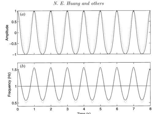
Its Hilbert transform is simply cost. The phase plot ofx–yis a simple circle of unit radius as in figure 1a. The phase function is a straight line as shown in figure 1b and the instantaneous frequency, shown in figure 1c, is a constant as expected. If we move the mean off by an amountα, say, then,
x(t) =α+ sint. (3.13)
c b a (a)
θ3 θ2 θ1
Phase angle (rad) frequency (rad s–1)
a
a
b
b
c
c
(b) (c)
Figure 1. Physical interpretation of instantaneous frequency. (a) The phase plane for the model functions ofx(t) =α+ sint. (a)α= 0; (b)α <1; (c)α >1. (b) The unwrapped phase function of the model functions. (c) The instantaneous frequency computed according to equation (3.4).
The phase plot ofx–y is still a simple circle independent of the value ofα, but the centre of the circle will be displaced by the amount ofα as illustrated in figure 1a.
If α <1, the centre is still within the circle. Under this condition, the function has already violated a restriction, for its Fourier spectrum has a DC term; nevertheless, the mean zero-crossing frequency is still the same as in the case forα= 0, but the phase function and the instantaneous frequency will be very different as shown in figures 1b, c. If α >1, the centre is outside the circle; thus, the function no longer satisfies the required conditions. Then both the phase function and the instantaneous frequency will assume negative values as shown in figures 1b, c, which are meaningless.
These simple examples illustrate physically that, for a simple signal such as a sine function, the instantaneous frequency can be defined only if we restrict the function to be symmetric locally with respect to the zero mean level.
For general data, any riding waves would be equivalent to the case ofα >1 locally;
any asymmetric wave form will be equivalent to the case of α < 1, but non-zero, locally. In order to have a meaningful instantaneous frequency, this local restriction should be used in lieu of the global requirements given previously. Furthermore, this local restriction also suggests a method to decompose the data into components for which the instantaneous frequency can be defined. The examples presented above, however, actually lead us to the definition of a class of functions, based on its local properties, designated as intrinsic mode function (IMF) for which the instantaneous frequency can be defined everywhere. The limitation of interest here is not on the existence of the Hilbert transform which is general and global, but on the existence of a meaningful instantaneous frequency which is restrictive and local.
4. Intrinsic mode functions
The simple examples given above provide more physical interpretation of the restrictive conditions; they also suggest a practical way to decompose the data so that the components all satisfy the conditions imposed on them. Physically, the nec- essary conditions for us to define a meaningful instantaneous frequency are that the functions are symmetric with respect to thelocal zero mean, and have the same num- bers of zero crossings and extrema. Based on these observations, we propose a class of functions designated as intrinsic mode functions here with the following formal definition.
An intrinsic mode function (IMF) is a function that satisfies two conditions: (1) in the whole data set, the number of extrema and the number of zero crossings must either equal or differ at most by one; and (2) at any point, the mean value of the envelope defined by the local maxima and the envelope defined by the local minima is zero.
The first condition is obvious; it is similar to the traditional narrow band require- ments for a stationary Gaussian process. The second condition is a new idea; it modifies the classical global requirement to a local one; it is necessary so that the instantaneous frequency will not have the unwanted fluctuations induced by asym- metric wave forms. Ideally, the requirement should be ‘the local mean of the data being zero’. For non-stationary data, the ‘local mean’ involves a ‘local time scale’ to compute the mean, which is impossible to define. As a surrogate, we use the local mean of the envelopes defined by the local maxima and the local minima to force the local symmetry instead. This is a necessary approximation to avoid the definition of a local averaging time scale. Although it will introduce an alias in the instantaneous frequency for nonlinearly deformed waves, the effects of nonlinearity are much weak- er in comparison with non-stationarity as we will discuss later. With the physical approach and the approximation adopted here, the method does not always guar- antee a perfect instantaneous frequency under all conditions. Nevertheless, we will show that, even under the worst conditions, the instantaneous frequency so defined is still consistent with the physics of the system studied.
The name ‘intrinsic mode function’ is adopted because it represents the oscillation mode imbedded in the data. With this definition, the IMF in each cycle, defined by the zero crossings, involves only one mode of oscillation, no complex riding waves are allowed. With this definition, an IMF is not restricted to a narrow band signal, and it can be both amplitude and frequency modulated. In fact, it can be non-stationary. As discussed above, purely frequency or amplitude modulated functions can be IMFs
Time (s) Wind speed (m s–1)
Figure 2. A typical intrinsic mode function with the same numbers of zero crossings and extrema, and symmetry of the upper and lower envelopes with respect to zero.
even though they have finite bandwidth according to the traditional definition. A typical IMF is shown in figure 2.
Having defined IMF, we will show that the definition given in equation (3.4) gives the best instantaneous frequency. An IMF after the Hilbert transform can be expressed as in equation (3.2). If we perform a Fourier transform on Z(t), we have
W(ω) = Z ∞
−∞a(t)eiθ(t)e−iωtdt,= Z ∞
−∞a(t)ei(θ(t)−ωt)dt. (4.1) Then by the stationary phase method (see, for example, Copson 1967), the maximum contribution toW(ω) is given by the frequency satisfying the condition
d
dt(θ(t)−ωt) = 0; (4.2)
therefore, equation (3.4) follows. Although mathematically, the application of the stationary phase method requires a large parameter for the exponential function, the adoption here can be justified if the frequency, ω, is high compared with the inversed local time scale of the amplitude variation. Therefore, this definition fits the best for gradually changing amplitude. Even with this condition, this is still a much better definition for instantaneous frequency than the zero-crossing frequency;
it is also better than the integral definition suggested by Cohen (1995) as given in equation (3.10). Furthermore, it agrees with the definition of frequency for the classic wave theory (see, for example, Whitham 1975).
As given in equation (4.2) and the simple analogy given in equations (3.2)–(3.4), the frequency defined through the stationary phase approximation agrees also with the best fit sinusoidal function locally; therefore, we do not need a whole oscillatory period to define a frequency value. We can define it for every point with the val- ue changing from point to point. In this sense, even a monotonic function can be treated as part of an oscillatory function and have instantaneous frequency assigned according to equation (3.4). Any frequency variation is designated as frequency mod- ulation. There are actually two types of frequency modulations: the interwave and the intrawave modulations. The first type is familiar to us; the frequency of the oscillation is gradually changing with the waves in a dispersive system. Technically, in the dispersive waves, the frequency is also changing within one wave, but that
was not emphasized either for convenience, or for lack of a more precise frequency definition. The second type is less familiar, but it is also a common phenomenon: if the frequency changes from time to time within a wave its profile can no longer be a simple sine or cosine function. Therefore, any wave-profile deformation from the simple sinusoidal form implies the intrawave frequency modulation. In the past such phenomena were treated as harmonic distortions. We will show in detail later that most such deformations are better viewed as intrawave frequency modulation, for the intrawave frequency modulation is more physical.
In order to use this unique definition of instantaneous frequency, we have to reduce an arbitrary data set into IMF components from which an instantaneous frequency value can be assigned to each IMF component. Consequently, for complicated data, we can have more than one instantaneous frequency at a time locally. We will intro- duce the empirical mode decomposition method to reduce the data into the needed IMFs.
5. The empirical mode decomposition method: the sifting process Knowing the well-behaved Hilbert transforms of the IMF components is only the starting point. Unfortunately, most of the data are not IMFs. At any given time, the data may involve more than one oscillatory mode; that is why the simple Hilbert transform cannot provide the full description of the frequency content for the general data as reported by Long et al. (1995). We have to decompose the data into IMF components. Here, we will introduce a new method to deal with both non-stationary and nonlinear data by decomposing the signal first, and discuss the physical mean- ing of this decomposition later. Contrary to almost all the previous methods, this new method is intuitive, direct, a posteriori and adaptive, with the basis of the decomposition based on, and derived from, the data.
The decomposition is based on the assumptions: (1) the signal has at least two extrema—one maximum and one minimum; (2) the characteristic time scale is defined by the time lapse between the extrema; and (3) if the data were totally devoid of extrema but contained only inflection points, then it can be differenti- ated once or more times to reveal the extrema. Final results can be obtained by integration(s) of the components.
The essence of the method is to identify the intrinsic oscillatory modes by their characteristic time scales in the data empirically, and then decompose the data accordingly. According to Drazin (1992), the first step of data analysis is to examine the data by eye. From this examination, one can immediately identify the different scales directly in two ways: by the time lapse between the successive alternations of local maxima and minima; and by the time lapse between the successive zero cross- ings. The interlaced local extrema and zero crossings give us the complicated data:
one undulation is riding on top of another, and they, in turn, are riding on still other undulations, and so on. Each of these undulations defines a characteristic scale of the data; it is intrinsic to the process. We have decided to adopt the time lapse between successive extrema as the definition of the time scale for the intrinsic oscillatory mode, because it not only gives a much finer resolution of the oscillatory modes, but also can be applied to data with non-zero mean, either all positive or all negative values, without zero crossings. A systematic way to extract them, designated as the sifting process, is described as follows.
(a)
(b)
(c) Wind speed m s–1Wind speed m s–1Wind speed m s–1
Time (s)
Figure 3. Illustration of the sifting processes: (a) the original data; (b) the data in thin solid line, with the upper and lower envelopes in dot-dashed lines and the mean in thick solid line;
(c) the difference between the data andm1. This is still not an IMF, for there are negative local maxima and positive minima suggesting riding waves.
By virtue of the IMF definition, the decomposition method can simply use the envelopes defined by the local maxima and minima separately. Once the extrema are identified, all the local maxima are connected by a cubic spline line as the upper envelope. Repeat the procedure for the local minima to produce the lower envelope.
The upper and lower envelopes should cover all the data between them. Their mean is designated asm1, and the difference between the data andm1is the first component, h1, i.e.
X(t)−m1=h1. (5.1)
The procedure is illustrated in figures 3a–c(figure 3a gives the data; figure 3bgives
(a)
(b) wind speed (ms–1)wind speed (ms–1)
Time (s)
Figure 4. Illustration of the effects of repeated sifting process: (a) after one more sifting of the result in figure 3c, the result is still asymmetric and still not a IMF; (b) after three siftings, the result is much improved, but more sifting needed to eliminate the asymmetry. The final IMF is shown in figure 2 after nine siftings.
the data in the thin solid line, the upper and the lower envelopes in the dot-dashed lines, and their mean in the thick solid line, which bisects the data very well; and fig- ure 3cgives the difference between the data and the local mean as in equation (5.1)).
Ideally,h1 should be an IMF, for the construction ofh1 described above seems to have been made to satisfy all the requirements of IMF. In reality, however, overshoots and undershoots are common, which can also generate new extrema, and shift or exaggerate the existing ones. The imperfection of the overshoots and undershoots can be found at the 4.6 and 4.7 s points in figure 3b. Their effects, however, are not direct, for it is the mean, not the envelopes, that will enter the sifting process.
Nevertheless, the problem is real. Even if the fitting is perfect, a gentle hump on a slope can be amplified to become a local extremum in changing the local zero from a rectangular to a curvilinear coordinate system. An example can be found for the hump between the 4.5 and 4.6 s range in the data in figure 3a. After the first round of sifting, the hump becomes a local maximum at the same time location as in figure 3c. New extrema generated in this way actually recover the proper modes lost in the initial examination. In fact, the sifting process can recover low-amplitude riding waves with repeated siftings.
Still another complication is that the envelope mean may be different from the true local mean for nonlinear data; consequently, some asymmetric wave forms can still exist no matter how many times the data are sifted. We have to accept this approximation as discussed before.
Other than these theoretical difficulties, on the practical side, serious problems of the spline fitting can occur near the ends, where the cubic spline fitting can have large swings. Left by themselves, the end swings can eventually propagate inward and corrupt the whole data span especially in the low-frequency components. We have devised a numerical method to eliminate the end effects; details will be given later.
At any rate, improving the spline fitting is absolutely necessary. Even with these problems, the sifting process can still extract the essential scales from the data.
The sifting process serves two purposes: to eliminate riding waves; and to make the wave-profiles more symmetric. Toward this end, the sifting process has to be repeated more times. In the second sifting process,h1 is treated as the data, then
h1−m11=h11. (5.2)
Figure 4ashows the much improved result after the second sifting, but there are still local maxima below the zero line. After another sifting, the result is given in figure 4b.
Now all the local maxima are positive, and all the local minima are negative, but many waves are still asymmetric. We can repeat this sifting procedurek times, until h1k is an IMF, that is
h1(k−1)−m1k=h1k, (5.3)
the result is shown in figure 2 after nine siftings. Then, it is designated as
c1=h1k, (5.4)
the first IMF component from the data.
As described above, the process is indeed like sifting: to separate the finest local mode from the data first based only on the characteristic time scale. The sifting process, however, has two effects: (a) to eliminate riding waves; and (b) to smooth uneven amplitudes.
While the first condition is absolutely necessary for the instantaneous frequency to be meaningful, the second condition is also necessary in case the neighbouring wave amplitudes have too large a disparity. Unfortunately, the second effect, when carried to the extreme, could obliterate the physically meaningful amplitude fluctuations.
Therefore, the sifting process should be applied with care, for carrying the process to an extreme could make the resulting IMF a pure frequency modulated signal of constant amplitude. To guarantee that the IMF components retain enough physical sense of both amplitude and frequency modulations, we have to determine a criterion for the sifting process to stop. This can be accomplished by limiting the size of the standard deviation, SD, computed from the two consecutive sifting results as
SD = XT
t=0
"
|(h1(k−1)(t)−h1k(t))|2 h21(k−1)(t)
#
. (5.5)
A typical value for SD can be set between 0.2 and 0.3. As a comparison, the two Fourier spectra, computed by shifting only five out of 1024 points from the same data, can have an equivalent SD of 0.2–0.3 calculated point-by-point. Therefore, a SD value of 0.2–0.3 for the sifting procedure is a very rigorous limitation for the difference between siftings.
Overall,c1 should contain the finest scale or the shortest period component of the signal. We can separatec1 from the rest of the data by
X(t)−c1=r1. (5.6)
Time (s) Wind speed (ms–1)
Figure 5. Calibrated wind data from a wind-wave tunnel.
Since the residue, r1, still contains information of longer period components, it is treated as the new data and subjected to the same sifting process as described above. This procedure can be repeated on all the subsequentrjs, and the result is
r1−c2=r2, . . . , rn−1−cn =rn. (5.7) The sifting process can be stopped by any of the following predetermined criteria:
either when the component, cn, or the residue,rn, becomes so small that it is less than the predetermined value of substantial consequence, or when the residue, rn, becomes a monotonic function from which no more IMF can be extracted. Even for data with zero mean, the final residue can still be different from zero; for data with a trend, then the final residue should be that trend. By summing up equations (5.6) and (5.7), we finally obtain
X(t) = Xn
i=1
ci+rn. (5.8)
Thus, we achieved a decomposition of the data inton-empirical modes, and a residue, rn, which can be either the mean trend or a constant. As discussed here, to apply the EMD method, a mean or zero reference is not required; EMD only needs the locations of the local extrema. The zero references for each component will be generated by the sifting process. Without the need of the zero reference, EMD eliminates the troublesome step of removing the mean values for the large DC term in data with non-zero mean, an unexpected benefit.
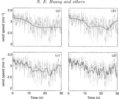
To illustrate the sifting process, we will use a set of wind data collected in a labo- ratory wind-wave tunnel (Huang & Long 1980) with a high-frequency response Pitot tube located 10 cm above the mean water level. The wind speed was recorded under the condition of the initial onset of water waves from a calm surface. Calibrated wind data are given in figure 5. Clearly, the data are quite complicated with many
Time (s)
C4C3C2C1u
(a)
Time (s)
C9C8C7C6C5
(b)
Figure 6. The resulting empirical mode decomposition components from the wind data: (a) the original data and the componentsc1–c4; (b) the componentsc5–c9. Notice the last component, c9, is not an IMF; it is the trend.
local extrema but no zero crossings, for the time series represents all positive num- bers. Although the mean can be treated as a zero reference, defining it is hard, for the whole process is transient. This example illustrates the advantage of adopting the successive extrema for defining the time scale; it also illustrates the difficulties of dealing with non-stationary data: even a meaningful mean is impossible to define, but for EMD this difficulty is eliminated. Figures 6a, b summarize all the IMF obtained from this repeated sifting processes. We have a total of nine components. Comparing this with the traditional Fourier expansion, one can immediately see the efficiency of the EMD: the expansion of a turbulence data set with only nine terms. From the result, one can see a general separation of the data into locally non-overlapping time scale components. In some components, such as c1 andc3, the signals are intermit- tent, then the neighbouring components might contain oscillations of the same scale, but signals of the same time scale would never occur at the same locations in two different IMF components.
Finally, let us examine the physical meaning of each IMF component. The com- ponents of the EMD are usually physical, for the characteristic scales are physical.
Nevertheless, this is not strictly true, for there are cases when a certain scale of a phenomenon is intermittent. Then, the decomposed component could contain two scales in one IMF component. Therefore, the physical meaning of the decomposition comes only in the totality of the decomposed components in the Hilbert spectrum.
Even with the entire set of decomposed components, sound physical interpretation is still not guaranteed for other decompositions such as Fourier expansion. Further discussions will be given later in detail. Having established the decomposition, we should check the completeness and orthogonality of this decomposition. Because this decomposition isa posteriori, the check should also bea posteriori.
6. Completeness and orthogonality
By virtue of the decomposition, completeness is given, for equation (5.8) is an identity. As a check of the completeness for the wind data numerically, we can recon- struct the data from the IMF components starting from the longest to the shortest periods in the sequence from figure 7a–j. Figure 7a gives the data and the longest period component,c9, which is the residue trend, not an IMF. By itself, the fitting of the trend is quite impressive, and it is very physical: the gradual decrease of the mean wind speed indicates the lack of drag from the calm surface initially and the increase of drag after the generation of wind waves. As the mean wind speed decreases, the amplitude of the fluctuation increases, another indication of wind–wave interactions.
If we add the next longest period component,c8, the trend of the sum,c9+c8, takes a remarkable turn, and the fitting to the data looks greatly improved as shown in figure 7b. By successively adding more components with increasing frequency, we have the results in the series of figures 7c–i. The gradual change from the monotonic trend to the final reconstruction is illustrative by itself. By the time we reach the sum of IMF components up to c3 in figure 7g, we essentially have recovered all the energy containing eddies already. The components with the highest frequencies add little more energy, but they make the data look more complicated. In fact, the high- est frequency component is probably not physical, for the digitizing rate of the Pitot tube is too slow to capture the high-frequency variations. As a result, the data are jagged artificially by the digitalizing steps at this frequency.
Time (s) Time (s) wind speed (ms–1)wind speed (ms–1)
(a) (b)
(c) (d)
Figure 7. Numerical proof of the completeness of the EMD through reconstruction of the original data from the IMF components. (a) Data (in the dotted line) and the c9 component (in the solid line).c9serves as a running mean, but it is not obtained from either mean or filtering. (b) Data (in the dotted line) and the sum ofc9–c8 components (in the solid line). (c) Data (in the dotted line) and the sum ofc9–c7 components (in the solid line). (d) Data (in the dotted line) and the sum ofc9–c6 components (in the solid line).
The difference between the reconstructed data from the sum of all the IMFs and the original data is shown in figure 7j, in which the maximum amplitude is less than 5×10⁻¹⁵, the roundoff error from the precision of the computer. Thus, the completeness is established both theoretically by equation (5.8), and numerically by figure 7j.
The orthogonality is satisfied in all practical sense, but it is not guaranteed theo- retically. Let us discuss the practical aspect first. By virtue of the decomposition, the elements should all be locally orthogonal to each other, for each element is obtained from the difference between the signal and its local mean through the maximal and minimal envelopes; therefore,
(x(t)−x(t))·x(t) = 0. (6.1)
Nevertheless, equation (6.1) is not strictly true, because the mean is computed via the envelopes, hence it is not the true mean. Furthermore, each successive IMF com- ponent is only part of the signal constitutingx(t). Because of these approximations, leakage is unavoidable. Any leakage, however, should be small.
The orthogonality of the EMD components should also be checked a posteriori numerically as follows: let us first write equation (5.8) as
X(t) =
n+1X
j=1
Cj(t), (6.2)
in which we have includedrn as an additional element. To check the orthogonality of the IMFs from EMD, we define an index based on the most intuitive way: first,
Time (s) Time (s)
Wind speed (ms–1) Wind speed ×10–15 (ms–1)
Wind speed (ms–1)Wind speed (ms–1) (e)
(g) (h)
(i) (j)
( f )
5
0
–5
0 10 20 30 0 10 20 30
Figure 7.Cont.(e) Data (in the dotted line) and the sum ofc9–c5components (in the solid line).
(f) Data (in the dotted line) and the sum ofc9–c4 components (in the solid line). (g) Data (in the dotted line) and the sum ofc9–c3 components (in the solid line). By now, we seem to have recovered all the energy containing eddies. (h) Data (in the dotted line) and the sum ofc9–c2
components (in the solid line). (i) Data (in the dotted line) and the sum ofc9–c1components (in the solid line). This is the final reconstruction of the data from the IMFs. It appears no different from the original data. (j) The difference between the original data and the reconstructed one;
the difference is the limit of the computational precision of the personal computer (PC) used.
let us form the square of the signal as X2(t) =n+1X
j=1
Cj2(t) + 2n+1X
j=1 n+1X
k=1
Cj(t)Ck(t). (6.3) If the decomposition is orthogonal, then the cross terms given in the second part on the right-hand side should be zero. With this expression, an overall index of orthogonality, IO, is defined as
IO =XT
t=0
n+1X
j=1 n+1X
k=1
Cj(t)Ck(t)/X2(t)
. (6.4)
For the wind data given above, the IO value is only 0.0067. Orthogonality can also
0 10 20
0 10 20 30
time (s)
frequency (Hz)
Figure 8. The Hilbert spectrum for the wind data with 200 frequency cells. The wind energy appears in skeleton lines representing each IMF.
time (s)
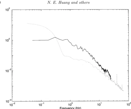
frequency (Hz)
0 10 20 30
0 10 20
Figure 9. The Morlet wavelet spectrum for the wind data with the same number of frequency cells. Wind energy appears in smoothed contours with a rich energy distribution in the high harmonics.
time (s)
frequency (Hz)
0 10 20 30
0 2 4 6 8 10
Figure 10. A 15×15 weighted Gaussian filtered Hilbert spectrum. The appearance gives a better comparison with the wavelet result, but the information content has been degraded.
be defined for any two components,Cf and Cg. The measure of orthogonality will, then, be
IOfg=X
t
CfCg
Cf2+Cg2. (6.5)
It should be noted that, although the definition of orthogonality seems to be global, the real meaning here applies only locally. For some special data, the neighbouring components could certainly have sections of data carrying the same frequency at different time durations. But locally, any two components should be orthogonal for all practical purposes. The amount of leakage usually depends on the length of data as well as the decomposition results. In reality, because of the finite data length, even pure sinusoidal components with different frequencies are not exactly orthogonal.
That is why the continuous wavelet in the most commonly used Morlet form suffers severe leakage. For the EMD method, we found the leakage to be typically less than 1%. For extremely short data, the leakage could be as high as 5%, which is comparable to that from a set of pure sinusoidal waves of the same data length.
Theoretically, the EMD method guarantees orthogonality only on the strength of equation (6.1). Orthogonality actually depends on the decomposition method. Let us consider two Stokian waves each having many harmonics. Separately, they are IMFs, of course, and each represents a free travelling wave. If the frequency of one Stokian wave coincides with the frequency of a harmonic of the other, then the two waves are no longer orthogonal in the Fourier sense. EMD, however, can still separate the two Stokian wave trains. Such a decomposition is physical, but the separated IMF components are not orthogonal. Therefore, orthogonality is a requirement only