Quantum Computing WS 2009/10

(1)

Quantum Computing WS 2009/10

Prof. Dr. Erich Grädel

Mathematische Grundlagen der Informatik RWTH Aachen

(2)

c b n d

This work is licensed under:

http://creativecommons.org/licenses/by-nc-nd/3.0/de/

Dieses Werk ist lizenziert unter:

http://creativecommons.org/licenses/by-nc-nd/3.0/de/

http://www.logic.rwth-aachen.de

1 Introduction

1.1 Historical overview

The history of quantum computing started in 1982 when Nobel laure- ate Richard Feynman argued that certain quantum mechanical effects cannot be simulated efficiently by classical computers. This started a debate whether these effects (in particular the parallelism which occurs inherently in quantum mechanical processes) could be employed by building a quantum computer.

Between 1985 and 1993, in a series of papers, Deutsch, Bernstein- Vazirani, Yao, and others advanced the theoretical foundations of quantum computing by providing theoretical models such as quantum Tur- ing machines and quantum gate arrays as well as introducing complex- ity classes for quantum computing and several simple algorithms that could be performed by a quantum computer.

A breakthrough occurred in 1994 when Peter Shor published his factorisation algorithm for quantum computers, which runs in poly- nomial time. His algorithm relies on the so-calledquantum Fourier transformation, which we will introduce later. Another example of a quantum algorithm is Grover’s search algorithm (1996), that can find a needle in a haystackof sizeNin time O(√

N).

Despite these surprising results, quantum computing still faces several problems: There are not many more algorithms known besides the one we have mentioned, and a quantum computer of moderate size that can keep a stable state for a sufficient amount of time needs yet to be built. So far, one was only able to build a quantum computer consisting of 7qubits, which successfully factorised the number 15=3·5.

(4)

1 Introduction

1.2 An experiment

The following experiment can be conducted using easily accessible ingredients:

• a powerful light source (e.g. alaser),

• three polarisation filters, which polarise light horizontally, verti- cally, and with an angle of 45°, respectively.

If we put one or more of the polarisation filters in front of the light source, we will make the following observations:

(1) If only the horizontal polarisation filter (→) is put in front of the light source, 50% of light passes through.

(2) If the vertical polarisation filter (↑) is put in front of the horizontal filter, 50% of light passes through the first filter, but the remaining light gets blocked by the second filter.

(3) However, if the diagonal filter (↗) is put between→and↑, we can observe that, from the total light emitted by the source, 50% passes through the first filter, 25% passes through the first two filters, and 12.5% of the light passes through all three filters, after all.

To explain these results, we describe the polarisation state of a photon by a vector

|φ⟩:=α|↑⟩+β|→⟩

in a 2-dimensional vector space with basis{|↑⟩,|→⟩}. Since the direc- tion of such a vector is all that matters, we only considerunit vectors:

|α|²+|β|² =1. Also note that the choice of the basis is arbitrary: In- stead of{|↑⟩,|→⟩}, one could also take{|↗⟩,|↘⟩}or, for that matter, any pair of orthogonal unit vectors.

Themeasurementof a state corresponds to the projection of such a vector with respect to an orthonormal basis, e.g.{|↑⟩,|→⟩}, which is given by the present equipment: If the vector|φ⟩=α|↑⟩+β|→⟩is measured, it is projected either to|↑⟩(with probability|α|²) or to|→⟩

(with probability|β|²).

1.3 Foundations of quantum mechanics

After the measurement, the vectorφis “destroyed”, i.e. it has been transformed into one of the basic states|↑⟩or|→⟩. There is no way to gain backφ, and each successive measurement gives the same result as the first one.

To each polarisation filter belongs a different orthonormal basis: If the angle of the filter isη, then the corresponding basis is

{sinη|↑⟩+cosη|→⟩, cosη|↑⟩ −sinη|→⟩}.

In particular, for both the horizontal and the vertical polarisation filter, the corresponding basis is{|↑⟩,|→⟩}, whereas for the diagonal filter↗, the basis is

{|↗⟩,|↘⟩}=ⁿ√¹

2(|↑⟩+|→⟩), 1

√2(|↑⟩ − |→⟩)^o

The photons that, after the measurement, correspond to the polarisation, pass through the filter; the others are reflected. Hence, filter→ projects 50% of the photons onto|→⟩and lets them pass; the other 50%

are projected onto|↑⟩and thus reflected. Filter↑, on the other hand, reflects all photons that are projected on|→⟩. Hence, no light passes through this filter if it is put behind filter→.

Filter↗projects a photon in state|→⟩= √¹

2|↗⟩ −^√¹₂|↘⟩with probability ¹₂ onto |↗⟩. Hence, if filter↗is put in between filter→ and filter↑, then 25% of the photons pass through the first two filters and are subsequently in state|↗⟩. Since|↗⟩= √¹

2|→⟩+√¹

2|↑⟩, half of these are projected by↑to|↑⟩and can pass through.

In general, astateis a complete description of a physical system. In quantum mechanics, a state is a unit vector in aHilbert space.

Definition 1.1. AHilbert space His a vector space over the fieldCof complex numbers, equipped with aninner product

⟨· | ·⟩:H×H→^C

(5)

1 Introduction

with the following properties:

• ⟨ψ|φ⟩=⟨φ|ψ⟩^∗for allψ,φ∈H(for a complex numberz=a+ib, itsconjugate z^∗is defined byz^∗=a−ib).

• ⟨ψ|ψ⟩ ≥0 for allψ∈H, and⟨ψ|ψ⟩=0 if and only ifψ=0 (the zero vector).

• ⟨ψ|αφ₁+βφ2⟩ = α⟨ψ|φ₁⟩+β⟨ψ|φ2⟩for all ψ,φ₁,φ2 ∈ H and α,β∈^C.

Note that, ifHis a Hilbert space, then∥·∥: H→^C, defined by

∥ψ∥:=^q⟨ψ|ψ⟩

for allψ∈H, defines anormonH.

Remark1.2. For Hilbert spaces of infinite dimension, in which we are not interested here, it is also required thatHiscomplete(with respect to∥·∥), i.e. that any Cauchy sequence has a limit.

In quantum mechanics, a vectorψ∈His usually written inDirac notationas|ψ⟩(readketψ). However, the zero vector is denoted by 0 (not|0⟩, which might be a different vector). For a given vector|ψ⟩, its dual vectoris denoted by⟨ψ|(readbraψ). Formally,⟨ψ|is the function fromHtoCthat maps a vector|φ⟩to the number⟨ψ|φ⟩.

Definition 1.3. Anorthonormal basis of a Hilbert space H is a basis {|e₁⟩, . . . ,|en⟩}ofHsuch that

⟨e_i|e_j⟩=





1 ifi=j, 0 ifi̸=j,

for alli,j=1, . . . ,n. In particular,∥e_i∥=1 for alli=1, . . . ,n.

The elementary building blocks of a classical computer are thebits, which can be in one of two states 0 or 1. In quantum computing, the elementary building blocks are thequbits; these are superpositions of two vectors|0⟩and|1⟩, which form a basis for the 2-dimensional Hilbert spaceH2. (Note that any two Hilbert spaces of the same dimension are isomorphic.)

Definition 1.4. Given a basis|0⟩,|1⟩ofH₂, aqubitis any vector|ψ⟩= α|0⟩+β|1⟩ ∈H²such that|α|²+|β|²=1.

Of course, a quantum computer will normally not only have access to one qubit but to many of them. A classical system with n bits comprises 2ⁿstates 0· · ·0, 0· · ·1 up to 1· · ·1. Ann-qubit system, on the other hand, has 2ⁿbasic states and can reside in any superposition

α0|0· · ·0⟩+α1|0· · ·1⟩+· · ·+α2ⁿ−1|1· · ·1⟩

such that∑²_i=0ⁿ⁻¹|αi|²=1. Such systems are also calledquantum registers.

Then-qubit spaceH2ⁿ can be obtained fromH2 by an operation called thetensor product. Formally, ifVandWare Hilbert spaces, then V⊗W(readV tensor W) is a Hilbert space of dimension dimV⊗W= dimV·dimW. Any two vectors|ψ⟩ ∈ V and|φ⟩ ∈ W correspond to a vector|ψ⟩ ⊗ |φ⟩ ∈V⊗W, and this operation is compatible with addition and scalar multiplication:

• (|ψ₁⟩+|ψ2⟩)⊗ |φ⟩=|ψ₁⟩ ⊗ |φ⟩+|ψ2⟩ ⊗ |φ⟩;

• |ψ⟩ ⊗(|φ₁⟩+|φ₂⟩) =|ψ⟩ ⊗ |φ₁⟩+|ψ⟩ ⊗ |φ₂⟩;

• α|ψ⟩ ⊗ |φ⟩=|ψ⟩ ⊗α|φ⟩=α(|ψ⟩ ⊗ |φ⟩).

In fact, if{v1, . . . ,vn}is a basis ofVand{w1, . . . ,wm}is a basis ofW, then{v_i⊗w_j : i=1, . . . ,n, j =1, . . . ,m}is a basis of V⊗W. Note that this space is different from theproduct space V×W, which is of dimension dimV+dimW. Instead of|ψ⟩ ⊗ |φ⟩, we also write|ψ⟩|φ⟩ or|ψφ⟩. We have

H2ⁿ=H2⊗ · · · ⊗H2

| {z }

ntimes

,

and {|0· · ·0⟩,|0· · ·1⟩, . . . ,|1· · ·1⟩} is a basis of H2ⁿ. Note that

(6)

1 Introduction

dimH₂ⁿ=2ⁿ. Hence, the dimension of the system grows exponentially in the number of qubits.

As opposed toH2×H2, not every state inH2⊗H2can be decom- posed into two states ofH2. We call such statesentangled.

Proposition 1.5. There exists a unit vector|ψ⟩ ∈ H2⊗H2 such that

|ψ⟩ ̸=|φ₁⟩ ⊗ |φ₂⟩for any two vectors|φ₁⟩,|φ₂⟩ ∈H₂.

Proof. Consider, for example,|ψ⟩:= √¹2(|00⟩+|11⟩), and assume that there exists|φ1⟩,|φ2⟩ ∈ H2 with|ψ⟩ =|φ1⟩ ⊗ |φ2⟩. Then there exist α₁,α₂,β₁,β₂∈^Csuch that|φ_i⟩=α_i|0⟩+β_i|1⟩fori=1, 2. Hence,

|ψ⟩= (α₁|0⟩+β₁|1⟩)⊗(α₂|0⟩+β₂|1⟩)

=α₁α₂|00⟩+α₁β₂|01⟩+α₂β₁|10⟩+β₁β₂|11⟩

Since{|00⟩,|01⟩,|10⟩,|11⟩}forms a basis ofH2⊗H2, we haveα₁β₂= α₂β₁=0. But then, alsoα₁α₂=0 orβ₁β₂=0, a contradiction. q.e.d.

In ann-qubit system, each qubit can be measured separately. The measurement of the first qubit of ann-qubit state|ψ⟩=_∑_v∈{0,1}nα_v|v⟩ can have two outcomes:

• With probabilityp=_∑_w_∈{_0,1_}n−1|α0w|², the result of the measurement is|0⟩, and|ψ⟩is projected onto the vector

|0⟩ ⊗√¹_p

∑

w∈{0,1}ⁿ⁻¹

α0w|w⟩.

• With probabilityq=∑_w∈{0,1}ⁿ⁻¹|α_1w|², the result of the measurement is|1⟩, and|ψ⟩is projected onto the vector

|1⟩ ⊗√¹_q

∑

w∈{0,1}ⁿ⁻¹

α_1w|w⟩.

A quantum-mechanical system evolves throughunitary transformations. Formally, a linear operatorU: H→H:|ψ⟩ 7→U|ψ⟩is unitary if it preserves the inner product:

⟨Uψ|Uφ⟩=⟨ψ|φ⟩

1.4 Quantum gates and quantum gate arrays

For the presentation of an operator by a matrixU⊆^Cⁿ^×ⁿthis means thatU^∗U =UU^∗ =I (the identity matrix), whereU^∗is theconjugate transposeofU, i.e. the matrix that results fromU by transposing U and replacing each entry by its conjugate. In particular, every unitary transformation is invertible, i.e.reversible.

Finally, we can postulate that any computation of a quantum computer consists of reversible building blocks (combined with mea- surements). This imposes a serious limitation on quantum computers.

For example, this implies that no quantum computer can simply copy around some qubits.

Theorem 1.6 (No-Cloning Theorem). Let H be any Hilbert space of dimensionn>1. There does not exist a unitary transformation Copy : H⊗H → H⊗H and a vector|0⟩ ∈ H such that Copy(|ψ⟩ ⊗ |0⟩) =

|ψ⟩ ⊗ |ψ⟩for allψ∈H.

Proof. Assume that Copy and|0⟩exist. Sincen>1, there exists a unit vector|1⟩that is orthogonal to|0⟩. Letψ= √¹

2(|0⟩+|1⟩). We have:

Copy(|ψ⟩|0⟩) = √¹

2(Copy(|0⟩|0⟩) +Copy(|1⟩|0⟩))

=√¹

2(|0⟩|0⟩+|1⟩|1⟩)

The latter vector is different from|ψ⟩|ψ⟩=¹₂(|00⟩+|01⟩+|10⟩+|11⟩),

a contradiction. q.e.d.

Definition 1.7. Aquantum gateon mqubits is a unitary transforma- tionU : H2^m → H2^m on the Hilbert space H2^m = H2⊗ · · · ⊗H2 of dimension 2^m.

Form=1, a quantum gate is a unitary transformationU:H₂→ H2. Consider the standard basis|0⟩,|1⟩ofH2. The transformationUis uniquely determined by its behaviour on the basis vectors:

U:|0⟩ 7→a|0⟩+b|1⟩

(7)

1 Introduction

|1⟩ 7→c|0⟩+d|1⟩,

As usual in linear algebra, we write these vectors as column vectors(_b^a) and(_d^c), respectively. Hence, the application ofUon the basis vectors

|0⟩= (¹₀)and|1⟩= (⁰₁)corresponds to a multiplication of the matrix a c

b d

!

with these vectors. ThatUis unitary is expressed by the matrix equation a^∗ b^∗

c^∗ d^∗

! a c b d

!

= ^{1 0} 0 1

!

Example1.8.

(1) Thenotgate is given by the matrix M_¬= ^{0 1}

1 0

! .

We haveM_¬|0⟩=|1⟩andM_¬|1⟩=|0⟩. (2) Consider the matrix

M= ¹ 2

1+i 1−i 1−i 1+i

! . Mis unitary since

M^∗M= ¹ 4

1−i 1+i 1+i 1−i

! 1+i 1−i 1−i 1+i

!

= ¹ 4

2(1−i²) (1−i)²+ (1+i)² (1−i)²+ (1+i)² 2(1−i²)

!

= ^{1 0} 0 1

! . Moreover, we have

M²=¹ 4

1+i 1−i 1−i 1+i

!2

= ^{0 1} 1 0

!

=M_¬. Hence,Mis a square root ofM_¬, and we writeM=√

M_¬. (3) TheHadamard transformationis given by the matrix

H= √¹ 2

1 1

1 −1

! .

It transforms the standard basis |0⟩,|1⟩ into the Hadamard basis (also called theFourier basis)

|0^′⟩=H|0⟩=√¹

2(|0⟩+|1⟩)

|1^′⟩=H|1⟩=√¹

2(|0⟩ − |1⟩) (see Section 1.2) and back:

H|0^′⟩=H 1/√

2 1/√

2

= 1

0

=|0⟩ H|1^′⟩=H1/√

2 1/√

2

= 0

1

=|1⟩

We denote the operation of a quantum gateUon 1 qubit as follows:

1 U

Other important gates on 1 qubit are S= ^{1 0}

0 i

!

(Phase) and

T= ¹ ⁰

0 e^iπ/4

! .

Note that S=T².

(8)

1 Introduction

Form =2, we are dealing with 2-qubit gates, which are of the formU:H4 →H4. The standard basis ofH4is|00⟩,|01⟩,|10⟩,|11⟩, or as coordinates

₁

00 0

,

₀

10 0

,

₀

01 0

,

₀

00 1

.

Example1.9. Thecontrolled notgate (cnot) is given by the matrix

Mcnot=







1 0 0 0 0 1 0 0 0 0 0 1 0 0 1 0







We have:

Mcnot|00⟩=|00⟩, Mcnot|01⟩=|01⟩, Mcnot|10⟩=|11⟩, Mcnot|11⟩=|10⟩.

Hence,Mcnot|ij⟩=|i⟩ ⊗ |i⊕j⟩(⊕denotesexclusive or, i.e.i⊕j=1 if and only ifi̸=j). The operation ofcnoton 2 qubits is denoted as follows:

1

2

In general, ifUis a unitary transformation on 1 qubit, then we can define a unitary transformationc-U(readcontrolled U) on 2 qubits as follows:

c-U|ij⟩=|i⟩ ⊗





U|j⟩ ifi=1,

|j⟩ ifi=0.

Graphically, this operation is denoted as follows:

1

2 U

IfUis represented by the matrix(_{b d}^{a c}), thenc-Uis represented by the matrix







1 0 0 0 0 1 0 0

0 0 a c

0 0 b d





.

Form=3, an interesting gate isc-cnot, better known as theToffoli gateTf, which is defined as follows:

Tf|ijk⟩=|ij⟩ ⊗ |ij⊕k⟩. The corresponding matrix is







1 0 0 0 0 0 0 0 0 1 0 0 0 0 0 0 0 0 1 0 0 0 0 0 0 0 0 1 0 0 0 0 0 0 0 0 1 0 0 0 0 0 0 0 0 1 0 0 0 0 0 0 0 0 0 1 0 0 0 0 0 0 1 0





 .

Graphically, this operation is denoted as follows:

1

2

3

(9)

1 Introduction

Of course, it is also possible to consider the Toffoli gate as a classical gate

Tf :{0, 1}³→ {0, 1}³: (i,j,k)7→(i,j,ij⊕k).

In fact, every classical circuit can be simulated by a circuit consisting of Tf gates only. For f :{0, 1}ⁿ→ {0, 1}ⁿconsider the reversible function f^′:{0, 1}ⁿ× {0, 1}ⁿ→ {0, 1}ⁿ× {0, 1}ⁿ:(x,y)7→(x,f(x)⊕y). We show that any reversible function can be computed by a circuit consisting of Tf gates.

More formally, we say that a setΩof reversible gates iscomplete (for classical reversible computation) if, given any reversible function g:{0, 1}ⁿ→ {0, 1}ⁿ, we can construct a circuit consisting of gates inΩ only that computes a functionh:{0, 1}ⁿ× {0, 1}^k→ {0, 1}ⁿ× {0, 1}^k such that for a fixedu∈ {0, 1}^kwe have

h(x,u) = (g(x),v) for allx∈ {0, 1}ⁿ.

Theorem 1.10. {Tf}is complete (for classical reversible computation).

Proof. We use the fact that every function can be computed by (classical) circuit consisting ofnandgates. Then, we can replace eachnandgate with inputsxandyby a Toffoli gate with inputsx,yand 1 (Note that xy⊕1=¬(x∧y)):

x

y ¬(x∧^y)

nand ⇝

x

y

1

x

y

xy⊕¹ Similarly, we can replace every branching with inputxby a Toffoli gate with inputs 1,xand 0 (Note thatx⊕0=x):

x

⇝ 1

x

0

1

x

x⊕⁰

q.e.d.

Recall thatc-UexecutesU on the target qubit if and only if the control qubit is set to 1:

1

2 U

We can switch the gate’s behaviour by introducing two¬gates:

1

2 U

= 1

2

¬ ¬

U

The resulting operation executesUif the control qubit is set to 0:

|ij⟩ 7→ |i⟩ ⊗





U|j⟩ ifj=0,

|j⟩ ifj=1.

Formally, the parallel execution of two unitary transformations corresponds to a tensor product of their matrices.

Definition 1.11. Let

A=







a₁₁ · · · a_1n ... ... am1 · · · amn





, B=







b₁₁ · · · b_1s ... ... ar1 · · · brs







(10)

1 Introduction

be two matrices of sizesm×nandr×s, respectively. The matrix

A⊗B:=







a11B a12B · · · a1nB a21B a22B · · · a2nB ... ... ... a_m1B a_m2B · · · amnB







of sizemr×nsis called thetensor productofAandB.

Proposition 1.12. Let Aand B be two 2×2 matrices that represent quantum gates on one qubit. Then, the simultaneous action ofAon the first andBon the second qubit is represented byA⊗B.

Proof. We have to check what the simultaneous action of AandBdoes to the basis vectors|00⟩,|01⟩,|10⟩and|11⟩ofH4. If

A= ^a⁰⁰ ^a⁰¹ a10 a11

!

andB= ^b⁰⁰ ^b⁰¹ b10 b11

! , then the basis vector|ij⟩is mapped to

A|i⟩ ⊗B|j⟩= (a_0i|0⟩+a_1i|1⟩)⊗(b_0j|0⟩+b_1j|1⟩)





 a_0ib_0j a0ib1j

a_1ib_0j a_1ib_1j







This is indeed the column that corresponds to|ij⟩in

A⊗B=







a00b00 a00b01 a01b00 a01b01

a₀₀b₁₀ a₀₀b₁₁ a₀₁b₁₀ a₀₁b₁₁ a₁₀b00 a₁₀b₀₁ a₁₁b00 a₁₁b₀₁ a10b10 a10b11 a11b10 a11b11





.

q.e.d.

This correspondence does not only hold for transformations onH2

but for transformation on any Hilbert space: IfAand Bare unitary transformation on two Hilbert spacesVandW, thenA⊗Bdefines the unitary transformation onV⊗Wthat corresponds to the simultaneous (or sequential) composition of Aand B(the order does not matter).

Moreover,A⊗Bdoes not introduce any entanglement.

Example1.13. LetA=B=H the Hadamard transformation. Then H⊗H=√¹

2

1 1

1 −1

!

⊗√¹ 2

1 1

1 −1

!

=¹ 2







1 1 1 1

1 −1 1 −1

1 1 −1 −1

1 −1 −1 1





,

and

(H⊗H)|ij⟩=¹

2 |00⟩+ (−1)^j|01⟩+ (−1)ⁱ|01⟩+ (−1)^i+j|11⟩

=¹

2 |0⟩+ (−1)ⁱ|1⟩)⊗(|0⟩+ (−1)^j|1⟩,

a non-entangled state, which is not a surprise given that |ij⟩ is not entangled and that H⊗H stands for the simultaneous action of H on each qubit.

On the other hand,Mcnot cannot be represented as a tensor product of two 2×2 matrices. To see this, consider the operation ofMcnot

on the non-entangled state|ψ⟩=√¹

2(|0⟩+|1⟩)⊗ |0⟩= √¹

2(|00⟩+|10⟩). We have Mcnot|ψ⟩ = √¹

2(|00⟩+|11⟩), and we know that this is an

(11)

1 Introduction

entangled state. Hence, Mcnot cannot possibly be equal to a tensor product of two 2×2 matrices.

Let us revisit the Hadamard transformation H, defined by the matrix

H= √¹ 2

1 1

1 −1

! , and consider the operation

H^⊗ⁿ=H| ⊗ · · · ⊗{z H}

ntimes

onnqubits. We have:

H^⊗n|0 . . . 0⟩=H|0⟩ ⊗ · · · ⊗H|0⟩

= √¹

2ⁿ (|0⟩+|1⟩)⊗ · · · ⊗(|0⟩+|1⟩)

= √¹ 2ⁿ

∑

x∈{0,1}ⁿ

|x⟩.

Hence, the first basis vector |0 . . . 0⟩ is transformed into a uniform superposition of all the 2ⁿbasis vectors. Graphically, this operation is denoted as follows:

1 2 ... n

H H ... H

Definition 1.14. Let Ω be a set of quantum gates. A quantum gate array (QGA) (or a quantum circuit) on n qubits over Ω is a unitary transformation, which is composed out of quantum gates inΩ.

Note that mathematically there is no difference between a quantum gate and a QGA: both are unitary transformations. The idea is that,

while a QGA may operate on a large number of qubits, a quantum gate may only operate on a small number of qubits.

The basic step in building a quantum gate array is letting a single gateUoperate on a selected number of qubits, say the qubitsi₁, . . . ,im. Mathematically, this operation (onnqubits) can be described by the unitary transformation

P⁻¹_i₁_...i_m(U⊗I₂^n−m)P_i₁_...i_m

where I₂^n−m is the identity mapping onH₂^n−mand P_i₁_...i_mis the transformation that permutes the qubits 1, . . . ,mwith the qubitsi₁, . . . ,im.

1 ... i1

... im

... n

U

Example1.15. Consider the following QGA consisting of Hadamard and cnotgates:

1

2

H H

The corresponding unitary transformation isU = H^⊗²·Mcnot·H^⊗². We claim thatU=P⁻¹₂₁ McnotP₂₁, the operation ofMcnoton the qubits 2 and 1 (instead of 1 and 2). LetM=Mcnot. Then:

U|ij⟩=H^⊗2·M1

2 |0⟩+ (−1)ⁱ|1⟩⊗ |0⟩+ (−1)^j|1⟩

=H^⊗²·M1

2 |00⟩+ (−1)^j|01⟩+ (−1)ⁱ|10⟩+ (−1)^i+j|11⟩

(12)

1 Introduction

=H^⊗²1

2 |00⟩+ (−1)^j|01⟩+ (−1)^i+j|10⟩+ (−1)ⁱ|11⟩

=H^⊗2H^⊗2 |i⊕j⟩ ⊗ |j⟩

=|i⊕j⟩ ⊗ |j⟩

2 Universal Quantum Gates

Consider then-arycontrolled operationcⁿ-Udefined by

cⁿ-U|i1. . .inj⟩=|i1. . .in⟩ ⊗





U|j⟩ ifi₁, . . . ,in=1,

|j⟩ otherwise.

How can we implement a complicated operation such ascⁿ-Uusing simple gates such as Tf andc-U? The idea is to introduce a certain number ofcontrol qubits, which are initially set to 0. Then, we can implementcⁿ-Uas follows (the right part of the array resets the work qubits to 0):

1 2 3 4 5

|⁰⟩

6 U

(13)

2 Universal Quantum Gates

In fact, we can build up the Toffoli gate Tf from the two-qubit gates c-V,c-V⁻¹andc-M_¬, where

V=√ M_¬=¹

2

1+i 1−i 1−i 1+i

! , as follows:

=

V V⁻¹ V

To see this, note that the gate on the right maps |ijk⟩ to |ij⟩ ⊗

|f(i,j,k)⟩, where

|f(i,j,k)⟩=











|k⟩ if|ij⟩=|00⟩, V⁻¹V|k⟩=|k⟩ if|ij⟩=|01⟩, VV⁻¹|k⟩=|k⟩ if|ij⟩=|10⟩, VV|k⟩=|k⊕1⟩ if|ij⟩=|11⟩

=|ij⊕k⟩.

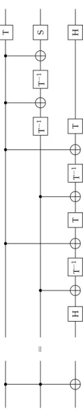
Lemma 2.1. Tf is computable by a QGA over{H,c-M_¬, S, T, T⁻¹}(see Figure 2.1).

Proof. By calculation. q.e.d.

The general question here is which gates are sufficient for building arbitrary unitary transformations. We will show that a QGA can be approximatedarbitrarily well by a QGA that consists of Hadamard,cnot and T gates only. More precisely, we will show that

(1) every unitary transformationUcan be written as a productU= Um. . .U₁of unitary operatorsU_ithat operate nontrivially only on a two-dimensional subspace ofH2ⁿ (generated by two vectors of the standard basis).

= HT−1TT−1

T−1 TH

T−1

T S

Figure 2.1.An implementation of the Toffoli gate over{H,c-M¬, S, T, T⁻¹}.

(14)

(2) every unitary transformation can be composed from cnot and quantum gates that operate on one qubit only;

(3) 1-qubit quantum gates can be approximated arbitrarily well using H and T.

To prove (1), consider a unitary transformationU : Hm → Hm

described by a unitary(m×m)-matrix.

Lemma 2.2. Uis a product of unitary matrices of the form







1...

1a c

1...

b 1d

1...

1





 .

Proof. Consider, for instance,m=3 and

U=







a d g b e h c f j





.

Ifb=0, setU1=I. Otherwise, set

U1=







a^∗ δ b^∗ b δ δ −^a_δ

1





,

whereδ=^p|a|²+|b|². The matrixU1is unitary, andU1·Uis of the form

U₁·U=







a^′ d^′ g^′ 0 e^′ h^′ c^′ f^′ j^′





.

Ifc^′=0, setU₂= a^{′ ∗}

11

. Otherwise, set

U2=_p ¹

|a^′|²+|c^′|²







a^′∗ 0 c^′∗

0 1 0

c^′ 0 −a^′





.

The matrixU₂U₁Uis unitary and of the form

U2U1U=







1 d^′′ g^′′

0 e^′′ h^′′

c^′ f^′′ j^′′





.

SinceU2U1Uis unitary, we haved^′′=g^′′=0. Finally, set

U3=





 1

e^′′∗ f^′′∗

h^′′∗ j^′′∗





.

We haveU3U2U1U=I, soU=U₁^∗U₂^∗U₃^∗, and eachU_i^∗is of the desired form.

In general, we are able to find matrixesU₁, . . . ,U_kof the desired form such thatU_k. . .U1U=I, wherek≤(m−1) + (m−2) +· · ·+1=

m(m−1)

2 . q.e.d.

Corollary 2.3. A unitary transformation onnqubits is equivalent to a product of at most 2ⁿ⁻¹(2ⁿ⁻¹−1) unitary matrices that operate nontrivially only on a 2-dimensional subspace ofH2ⁿ (generated by two vectors of the standard basis).

Remark2.4. The exponential blowup incurred by this translation is not avoidable.

We can now turn towards proving (2).

Lemma 2.5. Let U : H2ⁿ → H2ⁿ be a unitary transformation that operates nontrivially only on the subspace ofH₂ⁿ generated by|x⟩=

|x₁. . .xn⟩ and |y⟩ = |y₁. . .yn⟩. Then U is a product of cnot and 1-qubit gates.

(15)

Proof (Sketch). LetVbe the nontrivial, unitary(2×2)-submatrix ofU.

Vcan be viewed as a 1-qubit gate. Recall that, for eachn, the opera- tioncⁿ-Vcan be implemented using Tf (which can be built fromcnot and single qubit gates) andc-V. The gatec-V, on the other hand, can be implemented usingcnotand single qubit operations (see Nielsen &

Chuang,Quantum Computation and Quantum Information, Section 4.3).

Fix a sequence|z₁⟩, . . . ,|zm⟩of basis vectors such that|z₁⟩=|x⟩,

Finally, we can discuss (3), the reduction of arbitrary 1-qubit gates to H and T. Note that there exist uncountably many unitary transfor- mationsU :H2ⁿ →H2ⁿ, but from a finite (or even countably infinite) set of gates, we can only compose countably many QGAs. Hence, there is no way of representing every 1-qubit gateexactlyusing a fixed finite set of gates. However, an approximationis possible! For two unitary transformationsUandV, we define

E(U,V):= max

∥|ψ⟩∥=1∥(U−V)|ψ⟩∥.

Definition 2.6. A setΩof quantum gates isuniversalif for any QGAU and everyε>0, there is a QGAVconsisting only of gates fromΩsuch that E(U,V)≤ε.

Theorem 2.7(Solvay-Kitaev). For every QGAUconsisting ofmcnot or 1-qubit gates and for every ε > 0, there exists a QGAV of size O(m·log^{c m}_ε),c≈2, consisting ofcnot, H and T gates only such that E(U,V)≤ε.

3 Quantum Algorithms

3.1 The Deutsch-Jozsa algorithm

Suppose that your task is to decide whether a function f :{0, 1}ⁿ→ {0, 1}is either constantly equal to 0 or it isbalanced, i.e. f(x) =1 for precisely half of all inputsx∈ {0, 1}ⁿ(either one of these two cases is guaranteed to hold). If you decide correctly, you are awarded 1 000€.

On the other hand, a false answer is fatal. To help you find the right answer, you can repeatedly ask for the value of f for a given inputx.

Each such query will set you back 2€.

Classically, there is a good chance to find the right answer by drawing an inputxuniformly at random. Clearly, iff(x) =1, you can be sure that f is balanced. On the other hand, if f is balanced, then the probability that f(x) =0 forkinputs, chosen uniformly at random, is 1/2^k, which converges to 0 exponentially fast. However, unless you query more than 2ⁿ⁻¹ many inputs or get the answer that f(x) =1, you cannot be sure of your answer.

Suppose now that you may query a QGA on n+1 qubits for computing the functionU_f defined by¹

U_f|x⟩|j⟩=|x⟩|f(x)⊕j⟩.

Clearly, QGAs are more expensive than classical circuits, so let us say that each application ofU_f costs 500€. Can you get the correct answer and still make money in this case?

Surprisingly, the answer isyessince there exists a QGA that decides whether fis balanced with just one application ofU_f:

1Note thatUfhas to be unitary.

(16)

3 Quantum Algorithms

|0ⁿ⟩

|¹⟩

H^⊗ⁿ

H

U_f

H^⊗ⁿ

Measurement

Let us examine what the circuit does: First, the vector|0ⁿ⟩ ⊗ |1⟩is mapped by H^⊗n+1to

√1

2ⁿ⁺¹

∑

x∈{0,1}ⁿ

|x⟩ ⊗(|0⟩ − |1⟩).

Second, the QGA forU_fis applied to this vector, which yields the vector

√1

2ⁿ⁺¹

∑

x∈{0,1}ⁿ

|x⟩ ⊗(−1)^f(x)(|0⟩ − |1⟩)

=

∑

x∈{0,1}ⁿ

(−1√)^f^(x)|x⟩ 2ⁿ

⊗|0⟩ − |√ 1⟩ 2

=

∑

x∈{0,1}ⁿ

(−1)^f^(x)|x⟩

√2ⁿ

| {z }

=:|ψf⟩

⊗H|1⟩

To see what is the result of H^⊗ⁿ|ψ_f⟩, note that forx∈ {0, 1}, we can write H|x⟩as follows:

H|x⟩=√¹

2 |0⟩+ (−1)^x|1⟩

=√¹

2

∑

z∈{0,1}

(−1)^xz|z⟩.

Analogously, forx=x1· · ·xn∈ {0, 1}ⁿ, we have H^⊗ⁿ|x⟩= √¹

2ⁿ

∑

z=z1···zn∈{0,1}ⁿ

(−1)^x¹^z¹⁺^···^+xⁿ^zⁿ|z⟩

= √¹ 2ⁿ

∑

z∈{0,1}ⁿ

(−1)^x^·^z|z⟩.

3.2 Grover’s search algorithm

Hence,

H^⊗n|ψ_f⟩= √¹ 2ⁿ

∑

x∈{0,1}ⁿ

(−1)^f^(x)H^⊗n|x⟩

= ¹ 2ⁿ

∑

x∈{0,1}ⁿ

∑

z∈{0,1}ⁿ

(−1)^f^(x)+x·z|z⟩

= ¹ 2ⁿ

∑

z∈{0,1}ⁿ

∑

x∈{0,1}ⁿ

(−1)^f^(x)+x^·^z|z⟩.

In particular, the amplitude of the basis vector |0ⁿ⟩ in H^⊗ⁿ|ψ_f⟩ is

21ⁿ∑x∈{0,1}ⁿ(−1)^f^(x). If f ≡0, then this amplitude is equal to 1 and, with probability 1, the final measurement yields|0ⁿ⟩. On the other hand, if f is balanced, then the amplitude of|0ⁿ⟩is 0 and, with probability 1, the final measurement yields a basis vector different from|0ⁿ⟩.

While the Deutsch-Jozsa algorithm arguably solves an artificial problem, Grover’s algorithm solves a canonical search problem: This time, the task is to find, given an arbitrary Boolean function f :{0, 1}ⁿ→ {0, 1}, an inputxwith f(x) =1 (or to determine that there is no such input).

Classically, there is no better way than to test each input, which requires 2ⁿqueries to f in the worst case. Grover showed that if one has access to a QGA for computing the function

Uf :H₂ⁿ⁺¹ →H₂ⁿ⁺¹|x⟩ ⊗ |j⟩ 7→ |x⟩ ⊗ |f(x)⊕j⟩,

then one can build a quantum algorithm that finds anxwith f(x) =1 in time O(√

2ⁿ).

Our first approach is to apply a Hadamard transformation to|0ⁿ⟩to obtain a superposition of all inputs and then to applyU_f on H^⊗n|0ⁿ⟩ ⊗

|0⟩. The resulting vector is ψ:= √¹

2ⁿ

∑

x∈{0,1}ⁿ

|x⟩ ⊗ |f(x)⟩.

(17)

Can we measure|ψ⟩to find an inputxwith f(x) =1? For eachxwith f(x) =1, the amplitude of|x1⟩ in|ψ⟩is ^√¹₂_n. Hence, if for instance there is only one suchx, then a measurement ofψwill very likely not find this x. The idea of the algorithm is to apply a transformation on|ψ⟩that makes the amplitudes of the basis vectors|x1⟩much larger while making those of|x0⟩ smaller. After this transformation, with high probability a measurement of the last results in a basis vector of the form|x1⟩, i.e. f(x) =1. If the measurement fails and we obtain a vector|x0⟩, we just repeat the process.

It turns out that this idea can be made to work using a modified approach, where we applyU_f not to H^⊗n|0ⁿ⟩ ⊗ |0⟩, but to H^⊗n|0ⁿ⟩ ⊗ H|1⟩. As in the Deutsch-Jozsa algorithm, the resulting vector is|ψ_f⟩ ⊗ H|1⟩, where

|ψ_f⟩=

∑

x∈{0,1}ⁿ

(−1√)^f^(x)|x⟩ 2ⁿ .

LetV_f the transformation on the firstnqubits defined byU_f, œ Vf|x⟩= (−1)^f^(x)|x⟩.

For|ψ⟩=_∑_xax|x⟩, we have Vf|ψ⟩=

∑

x:f(x)=0

ax|x⟩ −

∑

x:f(x)=1

ax|x⟩.

For|ψ⟩=_∑_xax|x⟩, letA:=2⁻ⁿ∑xaxtheaverage amplitude. Consider the transformationDthat maps|ψ⟩to the vector∑x(2A−ax)|x⟩. The corresponding matrix is

D=







22ⁿ −1 ₂²n · · · ₂²n

22ⁿ 2

2ⁿ −1 ₂²n

... ... ...

22ⁿ 2

2ⁿ · · · ₂²ⁿ −1





 .

To see this, consider a basis vector|y⟩ =_∑_xδxy|x⟩ (whereδxy =1 if

x=yandδxy=0 otherwise). The average amplitude of|y⟩isA=₂¹n. Hence,D|y⟩= ₂²n−1

|y⟩+_∑_x̸=y₂²n|x⟩. Lemma 3.1. D=H^⊗ⁿ·Rn·H^⊗ⁿwith

Rn=







1−1

−1

...−1





.

Note thatRncan be implemented using O(n)simple gates.

Proof. Consider the matrix

R^′=Rn+In=





20

...0



.

We claim that

H^⊗ⁿ·R^′_n·H^⊗ⁿ= ² 2ⁿ





1 1··· 1 1 1··· 1

... ... ...

1 1··· 1



,

i.e. H^⊗n·R^′_n·H^⊗n|x⟩= ₂²n∑y|y⟩for allx∈ {0, 1}ⁿ:

|x⟩7−→^H^⊗n √¹ 2ⁿ

∑

z(−1)^x^·^z|z⟩

R^′n

7−→ √¹ 2ⁿ

∑

z(−1)^x·zR^′_n|z⟩= √² 2ⁿ|0⟩

H^⊗n

7−→ ₂²_n

∑

y |y⟩. Finally,

H^⊗n·Rn·H^⊗n=H^⊗n(R^′_n−In)H^⊗n

=H^⊗n·R^′_nH^⊗n−H^⊗n·In·H^⊗n

=H^⊗n·R^′_nH^⊗n−In

=D. q.e.d.

(18)

For a given functionf:{0, 1}ⁿ→ {0, 1}, Grover’s search algorithm iterates theGrover operator G:=D·V_f sufficiently oftenon input H^⊗ⁿ|0⟩ in order to magnify the amplitudes of the basis vectors|x⟩withf(x) =1.

But what do we mean bysufficiently often?

Consider the setsT={x: f(x) =1}andF={x: f(x) =0}. Af- ter r iterations ofG, the resulting vector will be of the form|ψr⟩ = tr∑x∈T|x⟩+ fr∑x∈F|x⟩ with average amplitude Ar = ₂¹n(−tr|T|+

fr(2ⁿ− |T|)). Now,

|ψr+1⟩=G|ψr⟩

=DV_f tr

∑

x∈T|x⟩+fr

∑

x∈F|x⟩

=D

−tr

∑

x∈T|x⟩+fr

∑

x∈F|x⟩

= (2Ar+tr)

∑

x∈T|x⟩+ (2Ar−fr)

∑

x∈F|x⟩. Hence,

t_r+1=2Ar+tr=1−²|T| 2ⁿ

tr+2−²|T| 2ⁿ

fr;

f_r+1=2Ar−fr=−²|T|

2ⁿ tr+1−²|T| 2ⁿ

fr.

This means that the coefficientstrand frsatisfy the following recursion:

t_r+1 fr+1

!

= ¹−δ 2−δ

−δ 1−δ

! tr

fr

!

, (3.1)

whereδ= ^2|T|₂n .

To compute the effect of the iterated application ofGon H^⊗ⁿ|0ⁿ⟩, we have to solve (3.1) under the initial conditiont₀= f₀= √¹

2ⁿ. Since G is unitary, we have ∥G|ψ⟩∥ = ∥ψ∥, i.e. |T|t²_r + (2ⁿ− |T|)f_r² = 1 for all r ∈ ^N. Hence, there exist ϑr such that tr = √¹

|T|sinϑr and fr= √ ¹

2ⁿ−|T|cosϑr.

The Grover operatorGcan be interpreted geometrically as a rota-

tion in the 2-dimensional space that is generated by the vectors

|φ⁺⟩= p¹

|T|

∑

x∈T|x⟩,

|φ⁻⟩= _p ¹ 2ⁿ− |T|

∑

x∈F|x⟩. We have

|ψ₀⟩= √¹ 2ⁿ

∑

x |x⟩

= r|T|

2ⁿ|φ⁺⟩+

r2ⁿ− |T| 2ⁿ |φ⁻⟩

=sinϑ₀|φ⁺⟩+cosϑ₀|φ⁻⟩.

Now, the Grover operator applied first performs a reflection across|φ⁻⟩ followed by a reflection across|ψ0⟩. The resulting operation is a rotation by 2ϑ0towards|φ⁺⟩. Hence,ϑr= (2r+1)ϑ0for allr∈^N.

In order for the final measurement to yield |x⟩ with x∈ T, we need thatϑr ≈ ^π₂ (so that|ψr⟩is close to|φ⁺⟩). Solving the equation (2r+1)ϑ0= ^π₂, we obtainr= _4ϑ^π₀−¹₂. Hence, forϑ0≈sinϑ0=

q|T|

2ⁿ, we can expect thatr =^π₄^q_|T|²ⁿ iterations suffice to find a solution with high probability. More precisely, we have the following theorem.

Theorem 3.2. Let f: {0, 1}ⁿ→ {0, 1}andm:=|{x: f(x) =1}|such that 0 < m ≤ ³₄ ·2ⁿ, and let ϑ0 < ^π₃ such that sinϑ0 = ₂^mn. After _π

4ϑ0

iterations ofG on |ψ0⟩ = √¹

2ⁿ ∑x∈{0,1}ⁿ|x⟩, a measurement of the resulting vector yields a basis vector|x⟩such that f(x) =1 with probability≥ ¹₄.

4ϑ0

= _4ϑ^π₀−¹₂+δ. Since|2δϑ0| ≤ |ϑ0| ≤ ^π₃, we

Quantum Computing WS 2009/10