Quantum Computing

(1)

Quantum Computing

Prof. Dr. Christoph Lehner

Lecture for Summer of 2020

(2)

(3)

Ideal quantum computing

1.1 Introduction to digital quantum computing

1.1.1 Qubits, gates, measurements

• A single qubit is a vector of unit length in the two-dimensional complex vector spaceS spanned by

|0i= 1

0

, |1i=

0 1

. (1.1)

• The direct product ofN vector spacesS creates the vector space S^N S^N ≡

ON i=1

S (1.2)

with dimensionality 2^N. A state ofN qubits is represented by a vector of unit length inS^N.

• Example: A two-qubit vector space is spanned by

|00i=





 1 0 0 0





, |01i=





 0 1 0 0





, |10i=





 0 0 1 0





, |11i=





 0 0 0 1





. (1.3)

• In general, thei-th component of a basis vector ofS^N will be written as (|bN−1bN−2· · ·b0i)i=

(1 fori=PN−1 j=0 bj2^j,

0 else (1.4)

with 0≤i <2^N. From left-to-right we therefore write the most-significant to least-significant bits. On occasion, we will write|iifor|bN−1bN−2· · ·b0i withi=PN−1

j=0 bj2^j and use the function bitj(i) =bj. 5

(6)

• A quantum gate is a unitary matrix acting onS^N.

• For a general state

|Ψi=

2X^N−1 i=0

Ψi|ii (1.5)

with Ψi∈CandP2^N−1

i=0 |Ψi|²= 1 we define Pj(|Ψi) =

2X^N−1 i=0;bitj(i)=1

|Ψi|² (1.6)

and a probabilistic measurement operation Mj :S^N →S^N ⊗ {0,1} that with likelihoodPj(|Ψi) maps|Ψito

Ψi

pPj(|Ψi)|ii ⊗1 (1.7) or else to

Ψi

p1−Pj(|Ψi)|ii ⊗0. (1.8) This operation therefore maps a qubit to a qubit and a classical bit in a probabilistic manner.

• The classical bit returned byMj is insensitive to a global complex phase of the state. This is important since the classical bits are the only way to extract information from the system. Global phases are therefore not important.

• A set of quantum gates that when combined can generate an arbitrary unitary matrix up to an arbitrary global phase is calleduniversal.

• A digital quantum computer is a machine that can apply quantum gates on N-qubit states and perform such measurements that provide a mapping to classical bits. Such a machine is called universal if it can apply a universal set of quantum gates.

1.1.2 Common one-qubit gates

• Hadamard

H = 1

√2

1 1 1 −1

(1.9) Action: |0i → ^√¹₂(|0i+|1i),|1i → ^√¹₂(|0i − |1i)

(7)

1.1. INTRODUCTION TO DIGITAL QUANTUM COMPUTING 7

• Phase shift gate

Rφ= 1 0

0 e^iφ

. (1.10)

Action: |0i → |0i,|1i →e^iφ|1i

• Pauli-X or NOT gate

X = NOT = 0 1

1 0

(1.11) Action: |0i → |1i,|1i → |0i

• Pauli-Y

Y =

0 −i i 0

(1.12) Action: |0i →i|1i,|1i → −i|0i

• Pauli-Z

Z= 1 0

0 −1

=Rπ (1.13)

• T =Rπ/4,S=Rπ/2

1.1.3 Common two-qubit gates

• Swap

SWAP =







1 0 0 0 0 0 1 0 0 1 0 0 0 0 0 1





 (1.14)

Action: |00i → |00i,|01i → |10i,|10i → |01i, |11i → |11i

• CNOT

CNOT =cX=







1 0 0 0 0 1 0 0 0 0 0 1 0 0 1 0





 (1.15)

Action: |00i → |00i,|01i → |01i,|10i → |11i, |11i → |10i;

Here: least-significant bit is target bit, most-significant bit is control bit Version for switched target and control bits in exercises.

(8)

1.1.4 Quantum circuits

• A quantum circuit is a specific combination of gates and measurements.

We introduce a graphical representation.

• A qubit is represented by a single line

|ψi

• N qubits may be grouped and written as

|ψi N

• A classical bit is represented by a double line bi

• The measurement of a qubit is represented as

|ψi bi

• A one-qubit gate operation is represented as

|ψi H

for the Hadamard gate and analog for other gates.

• The NOT gate has the special representation

|ψi

• Gate applications are read from left to right, so

|ψi A B

is represented as

BA|ψi (1.16)

in matrix notation.

• CNOT with least-significant target bit is represented as

(9)

|ψtargeti

|ψcontroli

One typically writes the least-significant qubit at the top. The case with least-significant control bit will be discussed in the exercises.

• A general controlled one-qubitU operation is represented as

|ψcontroli

|ψtargeti U

where U could, e.g., be H or Rφ, which is only applied to target bit if control bit is 1.

• SWAP is represented as

|ψi

|φi

1.1.5 Example: Bell states

The circuit

|0i H b0

|0i b1

performs the Bell experiment. After the Hadamard the system is in state

√1

2(|00i+|01i) (1.17)

and then after the CNOT in

√1

2(|00i+|11i). (1.18) The four possible classical results then are measured with probability

P(00) =P(11) = 1

2, P(10) =P(01) = 0. (1.19) The bits are maximally correlated and we always findb0=b1. Such correlation between qubits is called entanglement and is at the core of many quantum algorithms.

(10)

1.1.6 Quantum simulator

• A digital quantum computer can be simulated on a classical computer.

• On the course webpage, there is a link to http://github.com/lehner/sqc, a simple Python implementation of such a simulator; In this week’s exercises, we will discuss the usage of this library and we will use it to implement some of the algorithms introduced in the lecture.

• Caveat: with increasing number of qubits N, the problem size for the classical simulation increases as 2^N.

1.1.7 Many-qubit gates

• It is useful to define

√X =HRπ/2H =1 2

1 +i 1−i 1−i 1 +i

(1.20) with√

X√

X =X =NOT.

• Extend the CNOT gate by another control gate to the C²NOT or Toffoli gate. It can be implemented as

=

√X √

X^† √

X

• For controlled-U gate, replace √

X by √

U; see also problem set 2. For this, we will need

X^1/n=HRπ/nH . (1.21)

• Similarly the CⁿNOT can be obtained from the Cⁿ⁻¹NOT gate. For C³NOT

=

√X √

X^† √

X

With worker bits, we can implement this more efficiently, see problem set 2.

(11)

• We can also trigger on a 0 bit value by adding additional NOT gates. We write this with an empty circle

= X X

• Now we are ready to find a representation of a gate s^(ij) on S^N with s^(ij)|ii=|ji, s^(ij)|ji =|ii, s^(ij)|li=|li for 0≤i, j, l < 2^N and l 6=i, j.

This matrix plays a crucial role in the proof of universality done in the exercises

• Consider the bit-wise representation of i and j. Let i and j differ in n bits, then we can define so-called Gray codes gm, where g0 =i, gn =j, andgmandgm−1 only differ in one bit.

Example: i = 3 (011), j = 4 (100); g0 = 3 (011), g1 = 7 (111), g2 = 5 (101),g3= 4 (100)

• We can implements^(g^m^,g^m−1⁾by the C^N⁻¹NOT gate with target bit being the differing bit and triggering on the values of the common bits.

Example: g2= 5 andg3= 4 from above

3 3

s⁽⁵⁴⁾ =

• Then

s^(ij)=s^(g¹^,g⁰⁾· · ·s^(gⁿ⁻¹^,gⁿ⁻²⁾s^(gⁿ^,gⁿ⁻¹⁾· · ·s^(g¹^,g⁰⁾ (1.22) Example: i= 3,j= 4

3 3

s⁽³⁴⁾ =

(12)

1.1.8 Quantum parallelism

• For a general function

f :{0,1}^N → {0,1} (1.23) it will be useful to define

Uf :S^N ⊗S→S^N ⊗S,|xi ⊗ |yi 7→ |xi ⊗ |y⊕f(x)i, (1.24) where ⊕here means the modulo 2 operation. Such a function effectively evaluatesf for all possible values in parallel. We will also write|xi⊗|yi=

|x, yi. Note that the action on a general element ofS^N ⊗S is defined by the action on each basis element|x, yi.

• Since we cannot implement a non-reversible gate operation (quantum gates are unitary), we cannot map simply to|xi ⊗ |f(x)i. The simple reversible choice of y⊕f(x) will shown to be useful below.

• The circuit representation is

N N

|xi

Uf

|xi

|yi |y⊕f(x)i

• ForN = 1, the state

|Ψi= Ψ0,0|0,0i+ Ψ0,1|0,1i+ Ψ1,0|1,0i+ Ψ1,1|1,1i (1.25) then would be mapped to

Uf|Ψi= Ψ0,0|0,0⊕f(0)i+ Ψ0,1|0,1⊕f(0)i

+ Ψ1,0|1,0⊕f(1)i+ Ψ1,1|1,1⊕f(1)i. (1.26)

• Example: N = 1,f(x) = 1 We have

Uf|Ψi= Ψ0,0|0,1i+ Ψ0,1|0,0i+ Ψ1,0|1,1i+ Ψ1,1|1,0i. (1.27) or

Uf =

(13)

1.2. QUANTUM ALGORITHMS 13

• Example: N= 1, f(x) =x We have

Uf|Ψi= Ψ0,0|0,0i+ Ψ0,1|0,1i+ Ψ1,0|1,1i+ Ψ1,1|1,0i. (1.28) or

Uf =

1.2 Quantum algorithms

1.2.1 Deutsch–Jozsa algorithm

• A simple example for a problem that can be solved exponentially faster on a quantum computer than on a classical computer

• Problem: Given a function

f :{0,1}^N → {0,1} (1.29) that is either constant (maps always to either 0 or 1) or balanced (returns 0 for exactly half of the input domain and 1 else), find out if it is constant or balanced.

• Classical solution: evaluate function for all possible inputs and stop as soon as answer is known

– Best case: first two evaluations differ⇒function is balanced – Worst case: first 2^N⁻¹ evaluations are identical ⇒ answer known

after 2^N⁻¹+ 1 evaluations

– For randomized selection of inputs: probability of misidentification afternevaluations is≤2¹ⁿ

• Quantum algorithm (guaranteed result after one evaluation):

N N

|0i H^⊗^N

Uf

H^⊗^N r

|1i H

The measuredr = 0 if and only iff is constant. If f is balanced r6= 0 will be measured.

(14)

• Explanation:

We start with the input state (Mark states in diagram above)

Ψ0=|0i^⊗^N|1i. (1.30) After the Hadamard operations, we have

Ψ1=

2X^N−1 x=0

√ 1

2^N⁺¹|xi |0i − |1i

. (1.31)

To illustrate the mechanism, we remind ourself that forN = 2 (H⊗H)|00i= (H⊗1) 1

√2 |00i+|01i

, (1.32)

= 1

2 |00i+|10i+|01i+|11i

(1.33) and

H|1i= 1

√2 |0i − |1i

. (1.34)

ThenUf produces

Ψ2=

2X^N−1 x=0

√ 1

2^N⁺¹|xi |0⊕f(x)i − |1⊕f(x)i

(1.35)

=

2X^N−1 x=0

(−1)^f(x)

√2^N⁺¹ |xi |0i − |1i

. (1.36)

Next we note

H|bi= 1

√2 X1 b⁰=0

(−1)^bb⁰|b⁰i (1.37) withb∈ {0,1} or generally

H^⊗^N|xi= 1

√2^N

2X^N−1 z=0

(−1)^x^·^z|zi, (1.38) where

x·z≡





N−1X

j=0

bitj(x)bitj(z)



mod 2 (1.39)

and bitj(x) is the value of thej-th bit of x.

(15)

1.2. QUANTUM ALGORITHMS 15 Therefore the final state is

Ψ3=

2X^N−1 x,z=0

(−1)^z^·^x+f(x) 2^N |zi

|0i − |√ 1i 2

. (1.40)

Now iff(x) is constant, the amplitude of thez= 0 state is

2X^N−1 x=0

(−1)^f(x) 2^N

2

= 1 (1.41)

and therefore with certaintyr= 0 will be measured. If f(x) is balanced thez= 0 amplitude is

2X^N−1 x=0

(−1)^f(x) 2^N

2

= 0 (1.42)

and due to the normalization of the state a valuer6= 0 will be measured.

So with a single application of the quantum circuit, we know the answer.

• Run algorithm on sqc

(16)

1.2.2 Grover algorithm

• Problem:

Given a function

f :{0,1}^N → {0,1} (1.43) that is 1 for one value ofx0 with 0≤x0<2^N and 0 for all other values, findx0.

• Applications: Database search, cryptographic hash functions, factor n= p∗qwithpandqprime (classical test division up to√n)

• Classical solution requires O(2^N) evaluations of the function

• Here, we illustrate a quantum algorithm which requires O(√

2^N) function evaluations

• The quantum circuit is:

N N

|0i H^⊗N

G^k

r

|1i H

with

N N

G

=

N N

Uf

Us

and

Us = H^⊗^N 2|0i h0| −1 H^⊗^N .

• Fork≈√

2^N, we measurer=x0with high likelihood 1−O(1/2^N)

(17)

• Explanation:

We start with the input state (Mark states in diagram above)

Ψ0=|0i^⊗^N|1i. (1.44) After the Hadamard operations, we have

Ψ1=

2X^N−1 x=0

√ 1

2^N⁺¹|xi |0i − |1i

. (1.45)

Neglecting the trivial last qubit, we can say that at this point the system is in state

|ψi ≡ |ψ1i= 1

√2^N

2X^N−1 x=0

|xi=

r2^N−1

2^N |αi+ 1

√2^N |βi (1.46) with useful basis

|αi ≡ 1

√2^N −1 X

x6=x0

|xi, (1.47)

|βi ≡ |x0i. (1.48)

We will find that the remaining operations live in the space spanned by

|αiand|βi.

It is easy to verify thatUf :|xi |yi 7→ |xi |y⊕f(x)iperforms a reflection about|αiin this space, i.e.,

Uf(a|αi+b|βi) =a|αi −b|βi. (1.49) Similarly

cos(θ/2) =

r2^N −1

2^N (1.51)

or

θ= 2

√2^N

1 +O(1/2^N)

. (1.52)

Illustrate:

(18)

Figure 6.3. The action of a single Grover iteration,G: the state vector is rotated byθtowards the superposition

|β⟩of all solutions to the search problem. Initially, it is inclined at angleθ/2 from|α⟩, a state orthogonal to|β⟩.

An oracle operationOreflects the state about the state|α⟩, then the operation 2|ψ⟩⟨ψ| −Ireflects it about|ψ⟩.

In the figure|α⟩and|β⟩are lengthened slightly to reduce clutter (all states should be unit vectors). After repeated Grover iterations, the state vector gets close to|β⟩, at which point an observation in the computational basis outputs a solution to the search problem with high probability. The remarkable efficiency of the algorithm occurs becauseθbehaves likeΩ(!

M/N), so onlyO(!

N/M) applications ofGare required to rotate the state vector close to|β⟩.

whereθis a real number in the range 0 toπ/2 (assuming for simplicity that M≤N/2; this limitation will be lifted shortly), chosen so that

sinθ=2√ M(N−M)

N . (6.14)

6.1.4 Performance

How many times must the Grover iteration be repeated in order to rotate|ψ⟩near|β⟩? The initial state of the system is|ψ⟩=^!(N−M)/N|α⟩+^!M/N|β⟩, so rotating through arccos^!M/Nradians takes the system to|β⟩. Let CI(x) denote the integer closest to the real numberx, where by convention we round halves down, CI(3.5) = 3, for example. Then repeating the Grover iteration

R= CI

"

arccos^!M/N θ

#

(6.15) times rotates|ψ⟩to within an angleθ/2≤π/4 of|β⟩. Observation of the state in the computational basis then yields a solution to the search problem with probability at least one-half. Indeed, for specific values ofMandNit is possible to achieve a much higher probability of success. For example, whenM≪Nwe haveθ≈sinθ≈2^!M/N, and thus the angular error in the final state is at mostθ/2≈^!M/N, giving a probability of error of at mostM/N. Note thatRdepends on the number of solutionsM, but not

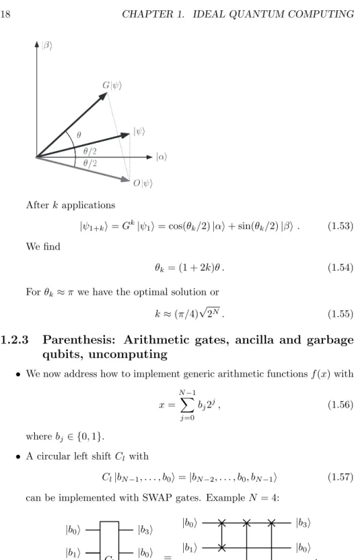
Afterk applications

|ψ1+ki=G^k|ψ1i= cos(θk/2)|αi+ sin(θk/2)|βi. (1.53) We find

θk= (1 + 2k)θ . (1.54)

Forθk ≈π we have the optimal solution or k≈(π/4)√

2^N. (1.55)

1.2.3 Parenthesis: Arithmetic gates, ancilla and garbage qubits, uncomputing

• We now address how to implement generic arithmetic functionsf(x) with x=

NX−1 j=0

bj2^j, (1.56)

where bj∈ {0,1}.

• A circular left shiftCl with

Cl|bN−1, . . . , b0i=|bN−2, . . . , b0, bN−1i (1.57) can be implemented with SWAP gates. ExampleN = 4:

|b0i Cl

|b3i

|b1i |b0i

|b2i |b1i

|b3i |b2i

=

|b0i |b3i

|b1i |b0i

|b2i |b1i

|b3i |b2i

.

(19)

1.2. QUANTUM ALGORITHMS 19 IfbN−1= 0, this implements

f(x) = 2x . (1.58)

If bN−1 = 1, the circular left shift results in an odd number, however, which we may not wish for an implementation off(x) = 2x.

• A left shift

Sl|bN−1, . . . , b0i=|bN−2, . . . , b0,0i (1.59) can be implemented if we add a so-calledancilla qubit with fixed value

|0ito the circuit, resulting in an additional variablegarbage qubit. We again illustrate forN= 4:

|b0i

Cl

|0i

|b1i |b0i

|b2i |b1i

|b3i |b2i

Ancilla qubit|0i |b3iGarbage qubit .

This operation again coincides withf(x) = 2x, however, has a more gra- cious overflow behavior (known from, e.g., C code) forbN−1= 1.

• A circular right shiftCr with

Cr|bN−1, . . . , b0i=|b0, bN−1, . . . , b1i (1.60) can again be implemented with SWAP gates. ExampleN = 4:

|b0i Cr

|b1i

|b1i |b2i

|b2i |b3i

|b3i |b0i

=

|b0i |b1i

|b1i |b2i

|b2i |b3i

|b3i |b0i

.

Ifb0= 0, this implements

f(x) =x/2. (1.61)

However forb0= 1 (for odd numbers), we do not obtain a sensible result for division by two.

(20)

• A right shift

Sr|bN−1, . . . , b0i=|0, bN−1, . . . , b1i (1.62) can again be implemented with ancilla and garbage qubits. We again illustrate forN = 4:

|b0i

Cr

|b1i

|b1i |b2i

|b2i |b3i

|b3i |0i

Ancilla qubit|0i |b0iGarbage qubit .

This operation coincides with f(x) =x/2 for allx.

• The need for ancilla and garbage qubits originates from the restriction to use reversible (unitary) gates on a quantum computer.

• Since the value of a garbage qubit is variable, we cannot reuse it as an ancilla bit for another gate. We can, however, use intermediate information and thenuncompute it to restore the ancilla bit.

Example: ImplementUf for

f(x) =

(1 for 2x= 10,

0 else . (1.63)

ForN = 4, this can be implemented as

|b0i

Uf

|b0i

|b1i |b1i

|b2i |b2i

|b3i |b3i

|0i |0i

|yi |y⊕f(x)i

=

(21)

|b0i

Cl Cr

|b0i

|b1i |b1i

|b2i |b2i

|b3i |b3i

|0i |0i

|yi |y⊕f(x)i

,

where the C⁴NOT operation only acts forx= 10 (binary 1010).

This “uncomputation” now allows for multiple applications of thisUf with only a single overall ancilla qubit.

• Next, we consider the function

f(x) =x+ 1. (1.64)

This can be implemented using elementary “half-adder” gates

|ai

O^+,1/2

|ai

|bi |a⊕bi= Sum Ancilla qubit|0i |abi= Carry

=

|ai |ai

|bi |a⊕bi

|0i |abi

.

We combine half-adders to implement the function. For N=3, e.g.,

(22)

|1i

O^+,1/2

|1i

|b0i |b⁰₀i

|0i

O^+,1/2

|b0i

|b1i |b⁰₁i

|0i

O^+,1/2

|b0b1i

|b2i |b⁰₂i

|0i |b0b1b2i

with

x+ 1 =

N−1X

j=0

b⁰_j2^j. (1.65)

• We can also add more generally

f(x) =x+z (1.66)

with

z=

NX−1 j=0

cj2^j. (1.67)

For this we need to define a full-adder gate

|ai

O⁺

|ai

|bi |bi

|ci |a⊕b⊕ci= Sum Ancilla qubit|0i |ab+c(a⊕b)i= Carry

=

|ai |ai

|bi |bi

|ci |a⊕b⊕ci

|0i |ab+c(a⊕b)i

.

(23)

1.2. QUANTUM ALGORITHMS 23 We combine full-adders to implement the function. For N=3, e.g.,

|0i

O⁺

|b0i

|c0i |b⁰₀i

|0i

O⁺

|b1i

|c1i |b⁰₁i

|0i

O⁺

|b2i

|c2i |b⁰₂i

|0i with

x+z=

NX−1 j=0

b⁰_j2^j, (1.68)

where we do not write the values of the garbage qubits.

• Similarly, we can implement subtraction.

• Finally, we consider multiplication ofxandz, i.e., f(x) =xz=

NX−1 j,j⁰=0

bjcj⁰2^j+j⁰ =

NX−1 j=0

bjS_l^j(z), (1.69)

where S^j_l(z) implements j left-shifts of the number z as defined above.

We note that we can implement binary multiplication as a combination of such shifts and addition.

1.2.4 Example: Solving an equation using Grover’s algo-

rithm

(24)

5/9/19, 1'23 PMgrover Page 1 of 20http://localhost:8888/nbconvert/html/grover.ipynb?download=false

In [1]:importsqc importnumpyasnp importmatplotlib.pyplotasplt

Contr ol-U gates (see also Pr oblem Set 2, Pr oblem 1)

In [2]:defA(i,o): returno.Rz(i,np.pi/4.0).H(i).Rz(i,np.pi/2.0) defAdg(i,o): returno.Rz(i,-np.pi/2.0).H(i).Rz(i,-np.pi/4.0) defCH(i,t,o):# i=control, t=target returnA(t,Adg(t,o).CNOT(i,t)) defCRz(i,t,phi,o): returno.Rz(t,phi/2.).CNOT(i,t).Rz(t,-phi/2.).Rz(i,phi/2.).CNOT(i, t) op=sqc.operator(2) foriinrange(4): st=sqc.state(2,v=[1ifi==jelse0forjinrange(4)]) print("Applying CH(0,1) to %s gives:\n%s\n"%(str(st),str(CH(0,1, op)*st))) print("Applying CRz(0,1,Pi/2) to %s gives:\n%s\n"%(str(st),str(C Rz(0,1,np.pi/2.,op)*st)))

5/9/19, grover Pagehttp://localhost:8888/nbconvert/html/grover.ipynb?download=false

gate (see also Lectur e Section 1.1.7) 𝐶

2

𝑋

(25)

In [3]:defCrootX(i,t,n,o): returnCH(i,t,CRz(i,t,np.pi/n,CH(i,t,o))) defCNOT(i,j,o): returno.CNOT(i,j) defC2rootX(i,j,t,n,o):#i,j=control; t=target returnCrootX(i,t,2.*n,CNOT(i,j,CrootX(j,t,-2.*n,CNOT(i,j,CrootX(j ,t,2.*n,o))))) op=sqc.operator(3) foriinrange(8): st=sqc.state(3,v=[1ifi==jelse0forjinrange(8)]) print("Applying C2NOT(0,1,2) to %s gives:\n%s\n"%(str(st),str(C2 rootX(0,1,2,1,op)*st)))

(see also Lectur e Section 1.1.7)

In Problem Set 02, we will learn a much faster implementation, that requires additional worker qubits.

𝐶

𝑛

𝑋

In [4]:defCnrootX(c,t,m,o):#c=array of n control qubits; t=target qubit assert(len(c)>0) iflen(c)==1: returnCrootX(c[0],t,m,o) i=[c[0]] j=[c[1]] r=c[2:] returnCnrootX(r+i,t,2.*m,CnrootX(r+i,j[0],1.,CnrootX(r+j,t,-2.* m,CnrootX(r+i,j[0],1.,CnrootX(r+j,t,2.*m,o))))) op=sqc.operator(4) foriinrange(16): st=sqc.state(4,v=[1ifi==jelse0forjinrange(16)]) print("Applying CnNOT([0,1,2],3) to %s gives:\n%s\n"%(str(st),st r(CnrootX([0,1,2],3,1,op)*st)))

(26)

5/9/19, grover Pagehttp://localhost:8888/nbconvert/html/grover.ipynb?download=false

Cir cular shift

In [5]:defSWAP(i,j,o): returno.CNOT(i,j).CNOT(j,i).CNOT(i,j) defCl(mask,o): foriinmask[1:]: o=SWAP(mask[0],i,o) returno defCr(mask,o): foriinreversed(mask[:-1]): o=SWAP(mask[-1],i,o) returno op=sqc.operator(4) st=sqc.state(4,v=[0,1]+[0]*14) foriinrange(4): print("Cl^%d |0001> = %s"%(i,str(st))) st=Cl([0,1,2],op)*st st=sqc.state(4,v=[0,1]+[0]*14) foriinrange(4): print("Cr^%d |0001> = %s"%(i,str(st))) st=Cr([0,1,2],op)*st

Gr over sear ch for 2x=10 (see Lectur e Section 1.2.2)

Cl^0 |0001> = 1 * |0001> Cl^1 |0001> = 1.0 * |0010> Cl^2 |0001> = 1.0 * |0100> Cl^3 |0001> = 1.0 * |0001> Cr^0 |0001> = 1 * |0001> Cr^1 |0001> = 1.0 * |0100> Cr^2 |0001> = 1.0 * |0010> Cr^3 |0001> = 1.0 * |0001>

(27)

In [6]:nqubits=4 expected_theta=2.*np.arccos(np.sqrt((2**nqubits-1.)/(2**nqubits))) optimal_k=int(np.round(np.pi/4.*np.sqrt(2**nqubits))) print("Optimal_k = %d"%optimal_k) plt.figure(figsize=(6,6)) plt.xlim(-1,1) plt.ylim(-1,1) plt.quiver([0],[0],[0,1],[1,0], color=['gray'],scale=3) plt.text(0.75,0,"|alpha>") plt.text(0,0.75,"|beta>") # TODO: theta_k plt.quiver([0],[0],[np.cos(expected_theta*(i+0.5))foriinrange(opti mal_k+1)], [np.sin(expected_theta*(i+0.5))foriinrange(optimal_k+1)], color=['r','b','g','black'],scale=4) plt.show() expected_theta_deg=expected_theta/np.pi*180. print("Optimal_angle = %g"%((optimal_k+0.5)*expected_theta_deg))

In [7]:print("Startup Grover Search") print("---") Nbits=nqubits+2# bits for x, 1 ancilla bit, 1 for y defpr(i,start,width): return(i//2**start)%(2**width) # Psi0 psi0=sqc.operator(Nbits).X(nqubits+1)*sqc.state(Nbits, basis=["|%d>|%d>|%d>"%(pr(i,0,nqubits),pr(i,nqubits,1), pr(i,nqubits+1,i))foriinrange(2**Nbits)]) print("|Psi0> = ") print(psi0) print("")# TODO: continue here # Psi1 psi1=sqc.operator(Nbits).H(0).H(1).H(2).H(3).H(5)*psi0 print("|Psi1> = ") print(psi1) print("")

Optimal_k = 3 Optimal_angle = 101.343

Quantum Computing