A Decision Support System for Photovoltaic Potential Estimation
Konstantin Hopf1 Michael Kormann1 Mariya Sodenkamp1 Thorsten Staake1,2
konstantin.hopf@uni-bamberg.de michael.kormann@gmx.de mariya.sodenkamp@uni-bamberg.de thorsten.staake@uni-bamberg.de 1) Management Information Systems / Energy Efficient Systems, University of Bamberg, 96045 Bamberg, Tel: +49 951 863 2236
2) Department of Management, Technology and Economics, ETH Zurich
ABSTRACT
With knowledge on the photovoltaic potential of individual residential buildings, solar companies, energy service providers and electric utilities can identify suitable customers for new PV installations and directly address them in renewable energy rollout and maintenance campaigns. However, many currently used solutions for the simulation of energy generation require detailed information about houses (roof tilt, shading, etc.) that is usually not available at scale. On the other hand, the methodologies enabling extraction of such details require costly remote-sensing data from three-dimensional (3D) laser scanners or aerial images.
To bridge this gap, we present a decision support system (DSS) that estimates the potential amount of electric energy that could be generated at a given location if a photovoltaic system would be installed. The DSS automatically generates insights about photovoltaic yields of individual roofs by analyzing freely available data sources, including the crowdsourced volunteered geospatial information systems OpenStreetMap and climate databases. The resulting estimates pose a valuable foundation for selecting the most prospective households (e.g., for personal visit and screening by an expert) and targeted solar panel kit offerings, ultimately leading to significant reduction of manual human efforts, and to cost-effective personalized renewables adoption.
CCS CONCEPTS
•Information systems~Decision support systems
•Information systems~Data analytics • Information systems~Location based services • Information systems~Data mining • Hardware~Renewable energy
KEYWORDS
Crowdsourced Data, Volunteered Geographic Information (VGI), Sensory Data, Data Analysis, Solar Potential, Photovoltaic, Renewable Energy
1 INTRODUCTION
Photovoltaic (PV) is one of the most promising energy suppliers in the future energy system and was the second-largest source of newly built renewable energy capacity in 2015 [26]. According to a recent study by Gagnon et al. [17], 39% of U.S. national electric- sector sales could be covered by PV installations on rooftops. By the end of 2015, the cumulative installed solar PV power capacity world-wide was 229 GW, but new investments decline currently due to the drop of subsidies (e.g., attractive incentive programs in Europe ended or will end in the near future) and concerns of investors on how fast renewables can be integrated in the grid infrastructure. These sorrows reduce the long-term investor conviction to invest in PV [25, 28, 53]. Nevertheless, the political will is to achieve large extension of renewables. For example, the EU members committed themselves to the binding goal that at least 27 % of consumed energy shall be produced by renewables by 2030 [13], in 2013 this portion was only 11.8% [14].
Rising energy prices in the future [57] will make PV investments profitable [4], and make them highly attractive for self-consumption or storage settings in residential home owners that can convert their rooftop into a profitable local solar plant already now.
One barrier for private investors to adopt solar installations on their rooftop is their unawareness of the actual potential of their home [55], because they are often unaware of the important determinants for the solar potential of their housing (different rooftop types, tilt, orientation, objects causing shadow, etc.) and how to evaluate the relevant variables for such an investment decision. On the other hand, PV providers go astray manually collecting and updating information about houses in the potentially appropriate areas. Thereby, knowledge on the solar PV potential of single residential building roofs is extremely valuable for solar companies, energy service providers and utilities. By having this location-based information for a large number of residencies energy companies can then select the most suitable households to promote new PV installations or maintenance support for already plugged-in solar panels. Furthermore, having these insights utilities and regional communities (including city planners and energy policy makers) can make more informed decisions about regional renewable energy strategies, better plan their local smart grid infrastructure development and design targeted green incentive campaigns [3, 61]. This will consequently lead to the increase of renewable energy share and support the achievement of ambitious sustainability goals.
Permission to make digital or hard copies of part or all of this work for personal or classroom use is granted without fee provided that copies are not made or distributed for profit or commercial advantage and that copies bear this notice and the full citation on the first page. Copyrights for third-party components of this work must be honored.
For all other uses, contact the owner/author(s).
IML '17, October 17-18, 2017, Liverpool, United Kingdom
© 2017 Copyright is held by the owner/author(s). Publication rights licensed to ACM.
ACM ISBN 978-1-4503-5243-7/17/10…$15.00 http://dx.doi.org/10.1145/3109761.3109764
2
The automatic prediction of the roof PV potential has been a subject to considerable amount of research, but existing studies rely on expensive data collection and are therefore regionally limited. The work presented in this paper goes beyond the state-of-the-art by presenting a new data-mining-based DSS that utilizes freely available sensory and crowdsourced Volunteered Geographic Information (VGI) data from OpenStreetMap as well as solar irradiation and temperature to automatically assess the PV potential of individual residential building roofs.
VGI digital data sources have emerged and millions of companies donate their information while users constantly generating new data online [9]. One prominent example is the project OpenStreetMap (OSM), that contains currently 3.8 billion entries on geographic places, streets, buildings, roads etc. [46].
Alongside preloaded digital maps from around the globe, the information within OSM is currently enhanced by a large group of volunteers who upload their sensory information such as satellite images, GPS tracks, but also field surveys to adjust and enrich the data for a region of interest. Some recent works already use OSM data for the PV potential prediction. In [31, 58] the total world solar energy potential on building roofs was estimated. Mainzer et al. [38] tested OSM data with satellite images to calculate the summarized areas of all building roofs in two cities
The methodology presented herein estimates a range of annual electricity energy (in kWh) that can be produced by a PV installation covering individual roofs. We combine several data mining related techniques to develop the decision support system [34]: our approach combines knowledge modeling with predictive analytics. Based on the location data of buildings and related unstructured crowdsourced geographic information [21, 65], we infer knowledge about private houses that is relevant for the PV potential estimation. On the other hand, quantitative domain- specific predictive models are applied for the roof area estimation and the amount of potentially generated PV energy at the given location. Thus, we apply knowledge on PV generation and geographic data to interpret and extract relevant features from OSM database, as well as use Monte-Carlo-Simulation [45] and mathematical models for electricity yield to estimate roof area and PV energy generation. From the engineering viewpoint, energy production yield across the roof was defined by Hookwijk [23]
which is the solar energy irradiated at the earth point (known as theoretical or geographical potential) lowered by several influence factors (e.g., conversion efficiency, shading, or losses due to cabling or transformation). The amount of PV power that is actually installed on building roofs can be lower than this estimated technical potential by considering non-technical aspects (e.g., available investment capital, subsidies, laws).
We have made four assumptions that are justified in the following sections: our approach works for residential buildings with (i) a rectangular basal area, that have (ii) a gabled rooftop with (iii) a tilt-angle of 35°. Besides that, (iv) structural limitations to the rooftop area (such as roof windows, antennas or chimneys) are not assessed individually (due to the lack of data), but included as averages.
This remainder of the paper is structured as follows: An overview to related work is given in the next section. We describe the methodology in Section 3. In Section 4, we show the results of validation with two real-world datasets, and in Section 5, we discuss possible improvements and current limitations.
2 LITERATURE REVIEW
Multiple studies suggest approaches for the prediction of the roof PV potential. The existing works rely upon various data sources with data granularities ranging from detailed three-dimensional data with a raster size of lower than 0.5m, raised in locally limited remote sensing studies [e.g., 33, 48], to globally aggregated statistics [e.g., 31, 58]. The data types include airborne Light Detection and Ranging (LiDAR) data, aerial images from satellite photogrammetry [47, 64], digital earth surface models [18], 3- dimensional (3D) building data [60] or two-dimensional (2D) cadaster data from official land surveying offices. An interested reader is referred to [5, 16, 41, 52] for detailed surveys on the PV potential estimation in urban landscapes. The existing approaches can be divided into four categories that we briefly describe below.
Constant-Value Methods: These works use generalized statistics (e.g., population, gross domestic product, construction statistics in a country) to roughly estimate the overall solar potential of larger regions [e.g., 36]. Due to the simplifications and assumptions, the methods are unsuitable to discriminate between individual buildings.
Manual Selection and Sampling Methods: Samples of rooftops from limited study areas are used to assess the typical solar potential of related buildings. The solar potential estimates for the selected rooftops are then calculated, based on aerial images, three-dimensional LiDAR data, or manual considerations, and the resulting estimate per building is extrapolated to the whole study region [e.g., 6, 47, 64]. Some works seek to draw correlations between population density and available roof area [e.g., 61] to support their estimation. Such manual sampling of houses and their solar potential assessment are hard to automate.
Solar potential estimation based on digital terrain models: Works in this category [e.g., 18, 31, 58] focus on the solar capabilities of complete regions with digital terrain models and environmental data (solar irradiation and weather), using geographic information software (such as ESRI ArcGIS, GRASS GIS, or others). The results are obviously more reliable than those from constant-value works, but assessment of individual roof solar potential is also not possible.
Solar potential estimation of individual roofs: Multiple studies on the solar potential of individual rooftops have been conducted, using 3-dimensional LiDAR data [e.g., 22, 27, 30, 33, 37, 44, 59]. The works rely on advanced cartographic collections from regionally limited remote sensing studies and show the possibility to assess the photovoltaic perspective for individual roofs at a high level of detail. Some authors [7, 12, 48, 49] even estimate the solar potential of building facades for vertical installations. These models achieve performance of up to 9% root-mean-square deviation from the real PV production figures [29]. However, these studies are regionally limited, since expensive data collection is
necessary. Moreover, solar companies and utilities usually do not have access to this kind of detailed data.
3 METHODOLOGY
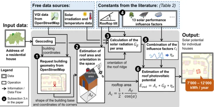
Figure 1 illustrates the decision support methodology, which encompasses six steps enumerated in the figure and consequently described in the following subsection. As an input, the artifact employs the postal address of a residential building. In addition, the method relies on freely available sensory and crowdsourced data: building geometries from OSM, solar irradiation and temperature. Further the model requires the values of parameters and influence factors (solar panel efficiency, roof shading etc.) to derive the expected range of PV yield on the rooftop per annum.
3.1 Retrieval of the building geometry from OpenStreetMap
At the initial stage, the shape of the building base as a polygon (specified by the coordinates of its corners) is retrieved from the OSM web service. After online request, the given address of the residency is converted to geocoded coordinates.
The data provided by the OSM web service consists of points and polylines on a 2D map, annotated with so called “tags”. These tags give semantic meaning to the objects (e.g., they identify lines as streets and polygons as buildings). Tags also contain further information to describe the geometries (e.g., street / building type, name, or opening hours of shops). Technically, tags are key-value pairs that users can add to objects. The OSM community maintains a comprehensive taxonomy of recommended tags, but the existence and quality of the tags associated with objects in the database varies to a large extend [1]. In our implementation, we select the closest building (polygon tagged with the key “building”) to the given location. Buildings with a larger Euclidean distance
than 50m to the location are excluded to avoid errors that are caused by the lack of data in OSM (this was the case in ca. 15% of our tested addresses).
The building type does not actually influence the roof area estimation, but we extract this information from OSM and use it in our validation. We distinguish thereby between residential buildings (that have an estimated rooftop area of lower than 400m2 and are tagged with the OSM key building, together with one of the values: apartments, detached, dwelling_house, house, residential, terrace semi_detached, semidetached_house,) and other buildings (e.g., commercial, industrial or unspecified buildings). For our purposes, only residential buildings are of interest.
3.2 Estimation of the rooftop area (𝑨𝒄) and orientation in the space (𝜷)
From the shape of the building base, we extract the rooftop area available for PV installations and the roof orientation in space.
The roof area is mainly determined by the roof type. Since roof type information is rarely existent in OSM [19] we consider the most frequent roof type gabled roof in official cadaster data (Table 1 shows the distribution of roof types based on [2] in a random sample of 3,627 buildings in Southern Germany). As the rooftop tilt, we consider 𝛼 = 35° for all buildings, according to previous studies [36].
We calculate the available rooftop area for solar installations 𝐴( with the building footprint area 𝐴) and the rooftop tilt 𝛼 [36]:
𝐴(=1 2∗ 𝐴)
cos 𝛼 (1)
In the VGI data, no structural limitations to the available rooftop area (like windows, antennas or chimneys) are included and therefore we leave them out in this study, because even in
Figure 1: Decision support methodology for estimating solar energy production potential of individual building roofs
4
studies using highly detailed 3D data, the exact identification of such limitations was not possible [30, 41].
Table 1: Roof types [2] and their frequency in a random sample of 3,627 buildings in Southern Germany.
Roof type Gabled roofs Flat roofs Other (11 types)
Frequency 2,328 540 759
Relative frequency 64% 15% 21%
To determine the roof ridge orientation, we use the building footprint corner coordinates, identify the longer side of the building and take the angle towards the sun, since a large majority of buildings are predominantly rectangular [54].
3.3 Computation of the amount of solar irradiation per area (',)
For the PV potential estimation, the amount of solar energy per area irradiated on the building roof and converted by PV modules to electrical energy is needed. We use Lamigueiro’s [32]
methodology and implementation that employs monthly solar radiation and temperature data at the specific location of the building (we use data from EUMETSAT [50]), together with the roof ridge orientation " and the roof tilt ! to calculate the amount of energy. Since the measurements are faced with inaccuracies and variations (local weather conditions, reflections, etc.), we use the 10-year average readings in order to get a general picture of the solar potential at a specific location.
3.4 Definition of the main features that influence PV yield
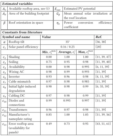
The conversion of the irradiated solar energy to electric energy that can be fed into the power grid is subject to losses. We conducted a comprehensive literature review to identify the factors that influence the PV electricity generation, and found 13 factors that we list Table 2 together with published statistics (min., average, max.).
Solar panel efficiency (0) refers to the percentage of solar energy that can be technically transformed into electricity by a PV installation. The PV panel efficiencies differ heavily between manufactures [63] and become more efficient with progress in the technical development. With the efficiency of up to 25%, silicon crystalline is today one of the most efficient solar panels. In our estimation, we assume an average efficiency of 16% which was a common standard in the year 2012 when the solar panels of our validation-data were installed [20].
The solar electric energy production is faced with environmental influences. First, shading (1) reflects what percentage of the roof area is shaded (e.g., by a tree or by neighboring buildings). Dust, snow and other soiling on the surface of a PV module (2) prevent solar radiation from reaching the solar cells thus lowering the efficiency. Furthermore, the
system shutdowns due to maintenance, grid outages, etc. reduce energy availability and output (3).
Besides that, technical losses lower the solar energy production. Within the solar cell where direct current (DC) electricity is produced, energy is lost due the wire connection between inverters, transformers and other parts of the installation (4). Inverter losses (5) happen during the conversion of DC in alternating current (AC) electricity mode. Cable mismatch (6) describes the electrical losses caused by slight differences of the manufacturing imperfections between modules in the array and different current-voltage characteristics. The initial light-induced degradation (7) describes the deposit of oxygen with silicon caused by a chemical process inside crystalline silicon solar cells during the photovoltaic effect. Further losses arise in the transportation of AC power (8), losses due to diodes (0/) and connections of the solar installation and of the transformers (00) are also considered in the literature.
Table 2: Variables and constants used in our methodology to estimate the PV potential of building roofs
Estimated variables
; Available rooftop area, see (1) EGF Estimated PV potential
= Area of the building footprint J Mean annual solar irradiation at the roof location
" Roof orientation in space #@ Power conversion efficiency coefficient
Constants from literature
Symbol and name Value Ref.
! Rooftop tilt 35° [36, 38]
0 Solar panel efficiency 0.16 / 0.25 [20]
Min, ACAD Average, A Max, AC>H
1 Shading 0.00 1.00 1.00 [11, 39, 47]
2 Soiling 0.75 0.95 0.98 [11, 39, 40]
3 Availability 0.00 0.98 0.995 [6, 11, 39]
4 Wiring AC 0.98 0.99 0.993 [11, 39]
5 Inverter 0.93 0.96 0.98 [4, 11, 39]
6 Cable mismatch 0.97 0.98 0.985 [11, 39]
7 Initial light-induced degradation
0.90 0.98 0.99 [6, 35, 39]
8 Cabling DC 0.97 0.98 0.99 [11, 39]
0/ Diodes and connections
0.99 0.995 0.997 [11, 39]
00 Transformers 0.96 0.97 0.98 [11, 39]
01 Manufacturer’s nameplate rating
0.85 1.00 1.05 [11, 39, 56]
02 Error rooftop area (availability for panels)
0.49 0.73 0.95 [43, 51, 61]
Finally, we consider two other coefficients. The manufacturer’s nameplate rating (01) is the differences between the solar panel efficiency figures published by the manufacturer and efficiency values that are measured under standard test conditions. The available rooftop has to be reduced due to structural limitations (e.g., windows, chimneys, antennas) by a ratio of the complete rooftop area and the area available for PV (02).
3.5 Definition of a cumulative performance measure (𝜼𝒆) based on Monte Carlo simulation
The identified influence factors must be combined to one single power conversion efficiency coefficient 𝜂G that is used in the PV potential estimation. A simple multiplication of all factors would ignore the distribution of each factor and leads to a large difference between the minimum and maximum estimated PV potential, due to the large range of some factors (e.g., 𝑐6, 𝑐8, 𝑐57).
Therefore, we use repeated random sampling for the aggregation of all influence factors 𝑐6, … , 𝑐57. This method is known as Monte Carlo simulation and has its application in math, physics, and business, when probabilistic problems with multiple variables must be solved [15].
In the Monte Carlo simulation, we assume all influence factors 𝑐6, … , 𝑐57 to be independent from each other and they can take a random value between 𝑐HIHJ and 𝑐HIKL, with the arithmetic mean of 𝑐H∗. The solar panel efficiency (𝑐5) is considered as a constant, because this factor depends on the technological state of the art and we use it as a parameter to the calculation. We approximate the cumulative density function 𝐶H 𝑥 for each coefficient stepwise, using the cumulative density function 𝐹U;W(𝑥) of the normal distribution 𝒩(𝜇, 𝜎6), where we define the mean as 𝜇 = 𝑐H∗, and the standard deviation by 𝜎IHJ;H=5[(𝑐H∗− 𝑐HIHJ) and 𝜎IKL;H=5[(𝑐HIKL− 𝑐H∗) according to 𝑐HIHJ and 𝑐HIKL; 𝑧 equals to the number standard deviations between 𝑐H∗ and 𝑐HIHJ / 𝑐HIKL:
𝐶H 𝑥 =
𝐹U;W^_`;_(𝑥) 𝑐H∗ 𝐹U;W^ab;_(𝑥)
: : :
𝑥 < 𝑐H∗ 𝑥 = 𝑐H∗
𝑥 > 𝑐H∗ (2) For the Monte Carlo simulation, we generated 10,000 independent random values for each influence factor, following the distribution 𝐶H 𝑥 that are within the range of the respective coefficient [𝑐HIHJ; 𝑐HIKL]. We calculate the aggregated influence factors 𝜂H∗ as the product Π of all coefficients, according to [6]:
𝜂H∗= 𝑐i Jj57
ij5
= 𝑐5∗ 𝑐6∗ … ∗ 𝑐J (3)
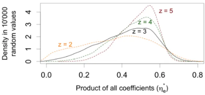
The resulting distribution of 𝜂H∗ is shown in Figure 2 for 𝑧 ∈ {2,3,4,5}. We choose 𝑧 = 3 for the use in our implementation, because 99.73% of all values in the normal distribution are within the interval of [𝜇 − 3𝜎; 𝜇 − 3𝜎] and the distribution of 𝜂G seems not to be overfitted.
As the result of the aggregated PV performance influence factors, we compute the power conversion efficiency coefficient 𝜂G as the expected value of the aggregated 𝜂H∗ values:
𝜂G = 1
10,000 5>r>>>𝜂H∗
Hj5 (4)
Figure 2: Distribution of the aggregated influence factors 𝜼𝒊∗ as a result of Monte Carlo simulation for different numbers of standard deviations (𝒛)
3.6 Roof photovoltaic potential estimation
To finally assess the electric energy 𝐸ABCthat can be generated by a PV installation and fed into the grid, we consider Hofierka and Kaňuk’s model [22] with three determinants (Equation 5):
Available rooftop area for solar cell installation 𝐴𝑐 (in m2), annual solar irradiation at the roof location 𝐺E (in Wh/m2), and mean annual power conversion efficiency coefficient (power input from the sun / power output from the system) 𝜂G from Equation 4.
𝐸ABC= 𝐴(∗ 𝐺E∗ 𝜂G (5) As an extension to Hofierka and Kaňuk’s [22] model, we express the vagueness of this estimation with an interval rather than with a single value and replace 𝜂G with an interval [𝜂G, 𝜂G] that contains 90% of the values for 𝜂H∗ (Equation 3). We define 𝜂G
as the 5%-quintile and 𝜂G as the 95%-quintile of the distribution of 𝜂H∗.Therefore, we provide an estimation of 𝐸ABCand a range of the PV production [𝐸ABC; 𝐸ABC].
4 VALIDATION
We make a two-fold validation of our approach. On the one hand, we validate our estimation of the rooftop area 𝐴( using official 3D cadaster data from the Bavarian land surveying office [2], containing detailed information on the roofs of 3,627 buildings. On the other hand, we validate our estimation of the possible PV electricity production 𝐸ABC using real-world production data from 85,806 existing solar collector installations throughout Germany [10]. Our primary focus in both validations lies – in line with the goal of this paper – in assessing the predictive quality of our method for the solar potential estimation of residential buildings with gabled rooftops. Therefore, we distinguish between these buildings and other buildings (e.g. industrial or unspecified building types), and other/flat rooftops, if this information is available to us. The locations of all validation data are illustrated in Figure 3. For both validations, we provide detailed dataset descriptions, followed by the results and an interpretation in the sections below.
6
Figure 3: Map of Germany showing the places for rooftop area validation and the locations of the PV installations considered for the validation of PV potential estimates
4.1 Validation of the rooftop area estimate
4.1.1 Validation dataset
The Bavarian land surveying office provided us with laser-scanned 3D cadaster-data for 𝑛v=3,627 houses located in three places in Southern Germany. We selected the places in cooperation with the land surveying office, following the motivation to include residential houses in the countryside, in villages and in suburbs, according to the categorization of Lödl et al. [36]. We chose therefore study areas that show different townscapes: Würzburg/
Altstadt is an old district area of a large town, Würzburg/Sanderau and Bamberg/Gartenstadt are newer districts of towns that are characterized by many residential buildings. In contrast, the village Moosach is a rural area with larger buildings and more open space.
The cadaster-data contains information on the buildings and the corresponding rooftops. Each building has one or more roofs associated. For each roof, the actual area 𝐴? and the roof type (see Table 1) is known.
4.1.2 Validation results
We validate the methodology for estimation of rooftop area by comparing the calculated area 𝐴(H (based on OSM data) with the true area 𝐴?w (based on cadaster data) and calculating the error δHv= 𝐴?H − 𝐴?w for each building 𝑖. As measure for the model performance, we use the mean absolute error 𝑀𝐴𝐸 =
5
J{ J{ δHv
Hj5 and the model bias error 𝑀𝐵𝐸 =J5
{ J{ δHv Hj5
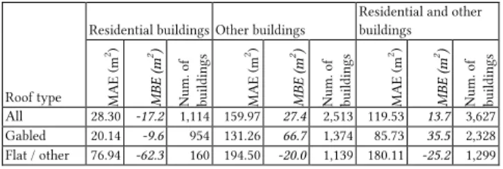
according to [62] and present the results in Table 3. Negative values of MBE indicate an underestimation. The results are separated by the building type (the categories residential buildings and other buildings are based on the OSM data, as we describe in Section 3.1) and the roof type (categories gabled rooftops and flat / other rooftops, based on the information from the cadaster data, as included in Table 1). Existing studies that estimate the PV suitable rooftop area only rarely validate their results with real world data. In the lack of such benchmarks, we consider two
random guess estimators (see Table 4) that we use to compare the MAE values with:
1. Random guess: This estimator assumes that all buildings have the same average rooftop size. In the lack of existing statistics on the roof area in Germany, we consider the average floor area of 91.4 m2 where residents in Germany are living on [8] and take the average rooftop area of 111.58 m2 (assuming a rooftop tilt of 35°) as a benchmark for the rooftop area estimation.
2. Biased random guess: This estimator assumes that all buildings with the same roof type to have equal roof areas. We take the average rooftop area in our cadaster validation dataset for each of the three rooftop types (gabled, flat, other) and take these values as the estimated rooftop area. We assume that the roof type is known. The MBE for all roofs is therefore 0.
In the main category of interest – residential buildings with a gabled rooftop – our algorithm has an average prediction error of 20.14 m2. This is 27% of the mean residential building rooftop area (gabled roofs) in our validation data. The estimation for flat/other roof types and other building types is less accurate.
Table 3: Performance of rooftop estimation based on OSM data for different building and rooftop types
Roof type
Residential buildings Other buildings
Residential and other buildings
MAE (m2) MBE (m2) Num. of buildings MAE (m2) MBE (m2) Num. of buildings MAE (m2) MBE (m2) Num. of buildings All 28.30 -17.2 1,114 159.97 27.4 2,513 119.53 13.7 3,627 Gabled 20.14 -9.6 954 131.26 66.7 1,374 85.73 35.5 2,328 Flat / other 76.94 -62.3 160 194.50 -20.0 1,139 180.11 -25.2 1,299
Table 4: Average rooftop area values and random guess estimator results for the rooftop area estimation
Random guess
Biased random guess gabled
roof
flat roof other roof types Average rooftop area (m2) 111.58 110.20 276.55 208.42 All buildings MAE (m2) 90.73 95.37
MBE (m2) -43.94 0
Residential buildings with gabled rooftop
MAE (m2) 49.91 48.94
MBE (m2) 36.79 35.41
4.1.3 Interpretation of the results
We interpret the performance of the rooftop area estimation for residential buildings with gabled roofs as good, considering the fact that the prediction is only based on 2D VGI data with a varying data quality [1]. Besides that, in a related study where OSM data was used together with satellite images, an error rate of 12-29% (amount of wrongly identified roof ridge lines) was achieved. In studies using 3D laser-scanning data, errors in the rooftop estimation of 15% are common [41, 61].
The roof area estimation for other buildings high errors and a large positive bias. We find two explanations for that: 1) entries in OSM are sometimes missing (some buildings are not mapped, so that the next building is considered by our implementation, and
many buildings have an unspecified type); 2) multiple houses are often mapped as one building (for example in the case of row houses, or semi-detached houses). One explanation for the underestimated roof area in the category of flat/other roofs lies in the used model (Equation 1) that is adapted to gabled roofs.
4.2 Validation of the solar potential estimate
4.2.1 Data description
We use real production data from existing PV installations in Germany for the second validation step. This data was recorded until 31.12.2013 for accounting the German Renewable Energies Act [66] subsidies and was made available online [10]. Besides the electric energy produced in 2013, the location, the year of construction, and the nominal installed capacity in kW-peak is known. We selected all PV installations on building roofs that have been built in 2012 (the 85,806 installations are depicted in Figure 3), which is the year before the data recording ended, since we assume that the newest installations represent the best technical state regarding to solar panel efficiency.
Some PV installations in the dataset have extreme large or low values that may distort our analysis. Therefore, we exclude about 4% of the data points as outliers that match the following criteria:
all installations with a real production higher than the 99% quintile (/88= 64,293 kWh), or lower than the 1% quintile (//0= 1,690 kWh), such as buildings with a predicted production that is higher than the 99% quintile (/88= 77,637 kWh), or lower than the 1%
quintile (/88= 623 kWh). Besides that, we exclude 14,092 installations that have no corresponding buildings mapped in the OSM database (as described in Section 3.1). In total, <V 71,330 installations are used for our validation.
4.2.2 Validation results
To validate the prediction of the photovoltaic potential, we compare the actual electrical energy production MEGF with the predicted solar potential EGFA . For each building , we compute the error A<V EGFA U EGFM and use VD0 DA90 A< and VD0 D A<
A90 as performance metrics.
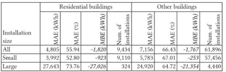
Table 5: Performance of the PV potential estimation model for different building types and installation sizes
Installation size
Residential buildings Other buildings
MAE (kWh) MAE (%) MBE (kWh) Num. of installations MAE (kWh) MAE (%) MBE (kWh) Num. of installations
All 4,805 55.94 -1,820 9,434 7,156 66.43 -1,767 61,896 Small 3,992 52.80 -923 9,110 5,783 67.01 -253 57,456 Large 27,643 73.76 -27,026 324 24,920 64.72 -21,354 4,440
The MAE of our PV potential estimation is 6,845 kWh (65.29%
of the average annual PV production in the complete validation dataset). The model underestimates the PV potential on average by 17% (MBE -1774 kWh). The detailed results for residential buildings and other buildings (the type was obtained from OSM, as described in Section 3.1) are shown in Table 5, separated by the
size of the PV installation (based on the nominal installed power in the validation data in small installations with Y30 kWp [66], and large installations).
4.2.3 Interpretation of the results
The average estimation error for the PV potential on residential building roofs is 55.15%. The error for small PV installations (Y30 kWp) is even lower at 52.27%.
The comparison of our validation results to the state of the art is difficult, because authors of PV potential studies lack frequently to validate their estimates with real production data [41]. Only Jakubiec and Reinhart [29] assess the performance of their algorithm for laser-scanning and daily solar irradiation data with two real roofs and found that they achieve 9% root-mean-square deviation from the real PV production figures. They also compare two other state of the art algorithms with their estimation and found that these estimations deviate by 32-37% in a test setting with 10 roofs. The results achieved in the test can therefore be interpreted as satisfactory, considering the quality and granularity of the underlying data (2D crowdsourced VGI data and averaged monthly solar irradiation and temperature).
5 LIMITATIONS AND IMPLICATIONS FOR FURTHER RESEARCH
Although the proposed DSS derives a good preliminary estimation of PV potential for individual residential building roofs, the following three limitations must be mentioned: First, the prediction quality depends heavily on the quality of the OSM data, that fortunately increases steadily [1], but in some regions data entries are still sparse. This leads to the problem that the yield prediction be made in particular cases due to the lack of data. In spite of this fact, our approach can be seen as an example for the quality assessment for VGI data based on application needs, as claimed by Mondzech and Sester [42]. Second, the approach is profiled to gabled building roofs with a tilt angle of 35°. Since flat roofs are also common, the parameters could be adjusted to provide also more accurate estimations for other roof types. Third, we included 13 influence factors and made assumptions on them (normal distribution of the factors, fixed value for the solar panel efficiency), that might have different distributions in specific regions (deserts, polar regions, etc.) or might change in the future.
Our implementation allows changing these values and adapting the method to other local conditions.
We believe, that our approach can be further extended with a more advanced querying of the building footprints from OSM. For that, a recently proposed algorithm by Hopf et al. [24] can be used, that selects OSM objects not only based on the distance, but also on semantics (objects tagged as residential buildings might be more applicable, even if they have a larger distance to the geo- located address, than objects tagged with greenhouse or garage).
Besides that, shadowing objects that are mapped in OSM, like trees or large buildings, or the sparsely recorded information on roof heights and roof types can be incorporated to provide a more accurate prediction of the solar energy assessment. Finally, our implementation could be further extended to provide estimations on further roof types to reduce estimation errors. For that, an
8
empirical study of existing roof types and the ability to recognize them from 2D data would be necessary.
6 CONCLUSION
In this paper, we presented a novel data-mining–based DSS that uses freely available crowdsourced data in combination with open sensory data (solar irradiation and temperature observations) to automatically assess the PV potential of individual residential building roofs. The estimation result can be used on large scale by solar companies, energy service providers and electric utility companies, supporting their decisions what (potential) residential customers to select for renewable energy rollout campaigns.
In the validation with cadaster data we found, that our approach obtains the rooftop area for residential gabled roofs based on 2D data with an error of 20.14 m2 (27% of the actual roof area). The validation of the PV potential estimation for residential buildings with real production data showed, that our method has an average error of 52%. For the initial assessment of the residential roof PV potential, without the use of costly and hard to obtain remote-sensing data (e.g., 3D laser-scanning data or aerial images) as used in previous works, the presented results are reasonable.
By going beyond the state of the art, this work makes both practical and theoretical contributions to the field of energy data analytics: Most importantly, we bridge the gap between the needs of solar energy companies to gain information about potential PV kit adopters and free broadly available VGI data. Moreover, this approach provides location-based PV yield estimations for the roofs at the individual level and is useable in manifold ways (for targeted marketing of solar energy providers, for personal decision support by household inhabitants, for policy preparation, etc.) Finally, this approach can be used for the quality assessment for VGI data based on the application needs [42]. All in all, this DSS is an obvious example of how crowdsourced and sensory data mining can contribute to the value generation for energy utilities, household residents and environmental sustainability.
Acknowledgements
The research presented in this paper was financially supported by Swiss Federal Office of Energy (Grant number SI/501202-01), and Eureka member countries and European Union (EUROSTARS Grant number E!9859 - BENgine II). We thank Denis Stühler for his contribution to implement an earlier version of the decision support system.
7 REFERENCES
[1] Ballatore, A. and Zipf, A. 2015. A Conceptual Quality Framework for Volunteered Geographic Information. Spatial Information Theory.
S.I. Fabrikant et al., eds. Springer International Publishing. 89–107.
[2] Bavarian Land Suveying Office 2015. Kundeninformation LoD2 (in German). Bayerisches Landesamt für Digitalisierung, Breitband und Vermessung.
[3] Branker, K. and Pearce, J.M. 2010. Financial return for government support of large-scale thin-film solar photovoltaic manufacturing in Canada. Energy Policy. 38, 8 (Aug. 2010), 4291–4303.
[4] Burger, B. et al. 2016. Photovoltaics Report. Frauenhofer ISE.
[5] Byrne, J. et al. 2015. A review of the solar city concept and methods to assess rooftop solar electric potential, with an illustrative application to the city of Seoul. Renewable and Sustainable Energy Reviews. 41, (Jan. 2015), 830–844.
[6] de Castro, C. et al. 2013. Global solar electric potential: A review of their technical and sustainable limits. Renewable and Sustainable Energy Reviews. 28, (Dec. 2013), 824–835.
[7] Catita, C. et al. 2014. Extending solar potential analysis in buildings to vertical facades. Computers & Geosciences. 66, (May 2014), 1–12.
[8] DESTATIS: Wohnungsbestand in Deutschland (in German): 2016.
https://www.destatis.de/. Accessed: 2016-08-26.
[9] Elwood, S. et al. 2012. Researching Volunteered Geographic Information: Spatial Data, Geographic Research, and New Social Practice. Annals of the Association of American Geographers. 102, 3 (Mai 2012), 571–590.
[10] EnergyMap - Auf dem Weg zu 100% EE - Der Datenbestand: 2015.
http://www.energymap.info/download.html. Accessed: 2016-02-20.
[11] Enphase Energy Inc. 2014. Guide to PVWatts Derate Factors for Enphase Systems When Using PV System Design Tools. National Renewable Energy Laboratory (NREL), Golden, CO.
[12] Esclapés, J. et al. 2014. A method to evaluate the adaptability of photovoltaic energy on urban façades. Solar Energy. 105, (2014), 414–427.
[13] European Commission 2014. Communication from the Commission to the European Parliament, the Council, the European Economic and Social Committee and the Committee of the Regions a Policy Framework for Climate and Energy in the Period from 2020 to 2030.
[14] Eurostat 2015. Consumption of energy - Statistics Explained.
Eurostat.
[15] Fishman, G. 2013. Monte Carlo: Concepts, Algorithms, and Applications. Springer Science & Business Media.
[16] Freitas, S. et al. 2015. Modelling solar potential in the urban environment: State-of-the-art review. Renewable and Sustainable Energy Reviews. 41, (Jan. 2015), 915–931.
[17] Gagnon, P. et al. 2016. Rooftop Solar Photovoltaic Technical Potential in the United States: A Detailed Assessment. Technical Report #NREL/TP-6A20-65298. National Renewable Energy Laboratory.
[18] Gherboudj, I. and Ghedira, H. 2016. Assessment of solar energy potential over the United Arab Emirates using remote sensing and weather forecast data. Renewable and Sustainable Energy Reviews.
55, (Mar. 2016), 1210–1224.
[19] Goetz, M. and Zipf, A. 2012. Towards defining a framework for the automatic derivation of 3D CityGML models from volunteered geographic information. International Journal of 3-D Information Modeling (IJ3DIM). 1, 2 (2012), 1–16.
[20] Green, M.A. et al. 2014. Solar cell efficiency tables (version 44): Solar cell efficiency tables. Progress in Photovoltaics: Research and Applications. 22, 7 (Jul. 2014), 701–710.
[21] Guo, D. and Mennis, J. 2009. Spatial data mining and geographic knowledge discovery—An introduction. Computers, Environment and Urban Systems. 33, 6 (Nov. 2009), 403–408.
[22] Hofierka, J. and Kaňuk, J. 2009. Assessment of photovoltaic potential in urban areas using open-source solar radiation tools. Renewable Energy. 34, 10 (Oct. 2009), 2206–2214.
[23] Hoogwijk, M.M. 2004. On the Global and Regional Potential of Renewable Energy Sources. University of Utrecht.
[24] Hopf, K. et al. 2015. Identifying the Geographical Scope of Prohibition Signs. COSIT 2015 (Santa Fe, NM: USA, 2015), 247–267.
[25] IEA 2014. Medium-Term Renewable Energy Market Report 2014:
Market Analysis and Forecasts to 2020.