Elsevier
I N V I T E D P A P E R
FAST F O U R I E R T R A N S F O R M S : A T U T O R I A L REVIEW A N D A STATE O F T H E ART
P. D U H A M E L
C N E T / P A B / R P E 38-40, Rue du General Leclerc, 92131 lssy les Moulineaux, France M. V E T T E R L I
Dept o f EE and CTR, S. W. Mudd Building, Columbia University, 500 W 120th Street, New York, NY10027, U.S.A.
Received 22 December 1988 Revised 30 October 1989
Abstract. The publication of the Cooley-Tukey fast Fourier transform (FIT) algorithm in 1965 has opened a new area in digital signal processing by reducing the order of complexity of some crucial computational tasks like Fourier transform and convolution from N 2 to N log2 N, where N is the problem size. The development of the major algorithms (Cooley-Tukey and split-radix FFT, prime factor algorithm and Winograd fast Fourier transform) is reviewed. Then, an attempt is made to indicate the state of the art on the subject, showing the standing of research, open problems and implementations.
Zusammenfassung. Die Publikation von Cooley-Tukey's schnellem Fourier Transformations Algorithmus in 1965 brachte eine neue Area in der digitalen Signalverarbeitung weil die Ordnung der Komplexit/it von gewissen zentralen Berechnungen, wie die Fourier Transformation und die digitale Faltung, von N 2 zu N log2 N reduziert wurden (wo N die Problemgr6sse darstellt). Die Entwicklung der wichtigsten Algorithmen (Cooley-Tukey und Split-Radix FIT, Prime Factor Algorithmus und Winograd's schneller Fourier Transformation) ist nachvollzogen. Dann wird versucht, den Stand des Feldes zu beschreiben, um zu zeigen wo die Forschung steht, was flir Probleme noch offenstehen, wie zum Beispiel in Implementierungen.
Rrsum4. La publication de l'algorithme de Cooley-Tukey pour la transformation de Fourier rapide a ouvert une nouvelle
~re dans le traitement num6rique des signaux, en r4duisant l'ordre de complexit6 de probl~mes cruciaux, comme la transformation de Fourier ou la convolution, de N 2 ~ N log2 N (oh N est la taille du probl~me). Le drvelopment des algorithmes principaux (Cooley-Tukey, split-radix FFT, algorithmes des facteurs premiers, et transform6e rapide de Winograd) est drcrit. Ensuite, l'&at de l'art est donn4, et on parle des probl~mes ouverts et des implantations.
Keywords. Fourier transforms, fast algorithms, computational complexity.
1. Introduction
Linear filtering and Fourier transforms are among the most fundamental operations in digital signal processing. However, their wide use makes their computational requirements a heavy burden in most applications. Direct computation of both
c o n v o l u t i o n a n d d i s c r e t e F o u r i e r t r a n s f o r m ( D F T ) r e q u i r e s o n t h e o r d e r o f N 2 o p e r a t i o n s w h e r e N is t h e f i l t e r l e n g t h o r t h e t r a n s f o r m size. T h e b r e a k - t h r o u g h o f t h e C o o l e y - T u k e y F F T c o m e s f r o m t h e f a c t t h a t i t b r i n g s t h e c o m p l e x i t y d o w n t o a n o r d e r o f N log2 N o p e r a t i o n s . B e c a u s e o f t h e c o n v o l - u t i o n p r o p e r t y o f t h e D F T , t h i s r e s u l t a p p l i e s t o 0165-1684/90/$3.50 © 1990, Elsevier Science Publishers B.V.
2 6 0 P. Duhamel, M. Vetterli / A tutorial on fast Fourier transforms
the convolution as well. Therefore, fast Fourier transform algorithms have played a key role in the widespread use o f digital signal processing in a variety o f applications like telecommunications, medical electronics, seismic processing, radar or radio astronomy to name but a few.
Among the numerous further developments that followed Cooley and Tukey's original contribu- tion, the fast Fourier transform introduced in 1976 by Winograd [54] stands out for achieving a new theoretical reduction in the order of the multipli- cative complexity. Interestingly, the Winograd algorithm uses convolutions to compute DFTs, an approach which is just the converse of the con- ventional method o f computing convolutions by means o f DFTs. What might look as a paradox at first sight actually shows the deep interrelation- ship that exists between convolutions and Fourier transforms.
Recently, the C o o l e y - T u k e y type algorithms have emerged again, not only because implementa- tions o f the Winograd algorithm have been disap- pointing, but also due to some recent developments leading to the so-called split-radix algorithm [27].
Attractive features o f this algorithm are both its low arithmetic complexity and its relatively simple structure.
Both the introduction o f digital signal processors and the availability o f large scale integration has influenced algorithm design. While in the sixties and early seventies, multiplication counts alone were taken into account, it is now understood that the number of addition and memory accesses in software, and the communication costs in hard- ware are at least as important.
The purpose o f this p a p e r is first to look back at twenty years o f developments since the C o o l e y - Tukey paper. Among the abundance o f literature (a bibliography o f more than 2500 titles has been published [33]), we will try to highlight only the key ideas. Then, we will attempt to describe the state of the art on the subject. It seems to be an appropriate time to do so, since on the one hand, the algorithms have now reached a certain matur- ity, and on the other hand, theoretical results on
Signal Processing
complexity allow us to evaluate how far we are from optimum solutions. Furthermore, on some issues, open questions will be indicated.
Let us point out that in this paper we shall concentrate strictly on the computation o f the dis- crete Fourier transform, and not discuss applica- tions. However, the tools that will be developed may be useful in other cases. For example, the polynomial products explained in Section 5.1 can immediately be applied to the derivation o f fast running F I R algorithms [73, 81].
The p a p e r is organized as follows.
Section 2 presents the history o f the ideas on fast Fourier transforms, from Gauss to the split- radix algorithm.
Section 3 shows the basic technique that under- lies all algorithms, namely the divide and conquer approach, showing that it always improves the performance o f a Fourier transform algorithm.
Section 4 considers Fourier transforms with twiddle factors, that is, the classic C o o l e y - T u k e y type schemes and the split-radix algorithm. These twiddle factors are unavoidable when the trans- form length is composite with non-coprime factors.
When the factors are coprime, the divide and con- quer scheme can be made such that twiddle factors do not appear.
This is the basis o f Section 5, which then presents Rader's algorithm for Fourier transforms o f prime lengths, and Winograd's method for computing convolutions. With these results established, Sec- tion 5 proceeds to describe both the prime factor algorithm (PFA) and the Winograd Fourier trans- form (WFTA).
Section 6 presents a comprehensive and critical survey o f the body o f algorithms introduced so far, then shows the theoretical limits of the com- plexity o f Fourier transforms, thus indicating the gaps that are left between theory and practical algorithms.
Structural issues of various F F T algorithms are discussed in Section 7.
Section 8 treats some other cases of interest, like transforms on special sequences (real or sym- metric) and related transforms, while Section 9 is
specifically devoted to the treatment of multi- dimensional transforms.
Finally, Section 10 outlines some of the impor- tant issues o f implementations. Considerations on software for general purpose computers, digital signal processors and vector processors are made.
Then, hardware implementations are addressed.
Some of the open questions when implementing F F T algorithms are indicated.
The presentation we have chosen here is con- structive, with the aim of motivating the 'tricks' that are used. Sometimes, a shorter but 'plug-in'- like presentation could have been chosen, but we avoided it, because we desired to insist on the mechanisms underlying all these algorithms. We have also chosen to avoid the use of some mathe- matical tools, such as tensor products (that are very useful when deriving some of the F F T algorithms) in order to be more widely readable.
Note that concerning arithmetic complexities, all sections will refer to synthetic tables giving the computational complexities of the various algorithms for which software is available. In a few cases, slightly better figures can be obtained, and this will be indicated.
For more convenience, the references are separ- ated between books and papers, the latter being further classified corresponding to subject mat- ters (1-D F F T algorithms, related ones, multi- dimensional transforms and implementations).
2. A historical perspective
The development of the fast Fourier transform will be surveyed below, because, on the one hand, its history abounds in interesting events, and on the other hand, the important steps correspond to parts o f algorithms that will be detailed later.
A first subsection describes the pre-Cooley- Tukey area, recalling that algorithms can get lost by lack o f use, or, more precisely, when they come too early to be o f immediate practical use.
The developments following the C o o l e y - T u k e y algorithm are then described up to the most recent
solutions. Another subsection is concerned with the steps that lead to the Winograd and to the prime factor algorithm, and finally, an attempt is made to briefly describe the current state o f the art.
2.1. From Gauss to the C o o l e y - T u k e y F F T While the publication of a fast algorithm for the D F T by Cooley and Tukey in 1965 [25] is certainly a turning point in the literature on the subject, the divide and conquer approach itself dates back to Gauss as noted in a well documented analysis by Heideman et al. [34]. Nevertheless, Gauss's work on FFTs in the early 19th century (around 1805) remained largely unnoticed because it was only published in Latin and this after his death.
Gauss used the divide and conquer approach in the same way as Cooley and Tukey have published it later in order to evaluate trigonometric series, but his work pre-dates even Fourier's work on harmonic analysis (1807)! Note that his algorithm is quite general, since it is explained for transforms on sequences with lengths equal to any composite integer.
During the 19th century, efficient methods for evaluating Fourier series appeared independently at least three times [33], but were restricted on lengths and number of resulting points. In 1903, Runge derived an algorithm for lengths equal to powers o f 2 which was generalized to powers o f 3 as well and used in the forties. Runge's work was thus quite well-known, but nevertheless disap- peared after the war.
Another important result useful in the most recent F F T algorithms is another type of divide and conquer approach, where the initial problem o f length N1" N2 is divided into subproblems of lengths N1 and N2 without any additional operations, N~ and N2 being coprime.
This result dates back to the work of G o o d [32]
who obtained this result by simple index mappings.
Nevertheless, the full implication o f this result will only appear later, when efficient methods will be derived for the evaluation o f small, prime length DFTs. This mapping itself can be seen as an
VoL 19, No. 4, April 1990
262 P. Duhamel, M. Vetterli / A
application of the Chinese remainder theorem (CRT), which dates back to 100 years A.D.!
[10.18].
Then, in 1965, appears a brief article by Cooley and Tukey, entitled 'An algorithm for the machine calculation o f complex Fourier series' [25], which reduces the order o f the n u m b e r o f operations from
N 2 t o N log2 ( N ) for a length N -- 2 n DFT.
This will turn out to be a milestone in the literature on fast transforms, and will even be credited [14, 15] of the tremendous increase o f interest in DSP beginning in the seventies. The algorithm is suited for DFTs on any composite length, and is thus o f the type that Gauss had derived almost 150 years before. Note that all algorithms published in-between were more restrictive on the transform length [34].
Looking back at this brief history, one may won- der why all previous algorithms had disappeared or remained unnoticed, whereas the C o o l e y - T u k e y algorithm had such a tremendous success. A poss- ible explanation is that the growing interest in the theoretical aspects o f digital signal processing was motivated by technical improvements in the semi- conductor technology. And, o f course, this was not a one-way street . . . .
The availability o f reasonable computing power produced a situation where such an algorithm would suddenly allow numerous new applications.
Considering this history, one may wonder how many other algorithms or ideas are just sleeping in some notebook or obscure publication . . . .
The two types of divide and conquer approaches cited above produced two main classes o f algo- rithms. For the sake o f clarity, we will now skip the chronological order and consider the evolution o f each class separately.
2.2. Development of the twiddle factor FFT When the initial D F T is divided into sublengths which are not coprime, the divide and conquer approach as proposed by Cooley and Tukey leads to auxiliary complex multiplications, initially named twiddle factors, which cannot be avoided in this case.
Signal Processing
tutorial on fast Fourier transforms
While Cooley-Tukey's algorithm is suited for any composite length, and explained in [25] in a general form, the authors gave an example with N = 2", thus deriving what is now called a radix-2 decimation in time (DIT) algorithm (the input sequence is divided into decimated subsequences having different phases). Later, it was often falsely assumed that the initial C o o l e y - T u k e y F F T was a D I T radix-2 algorithm only.
A n u m b e r of subsequent papers presented refinements o f the original algorithm, with the aim o f increasing its usefulness.
The following refinements were concerned:
- - w i t h the structure o f the algorithm: it was emphasized that a dual approach leads to 'decima- tion in frequency' (DIF) algorithms,
- - o r with the efficiency o f the algorithm, meas- ured in terms of arithmetic operations: Bergland showed that higher radices, for example radix-8, could be more efficient [21],
- - o r with the extension o f the applicability o f the algorithm: Bergland, again, showed that the F F T could be specialized to real input data [60], and Singleton gave a mixed radix F F T suitable for arbitrary composite lengths.
While these contributions all improved the initial algorithm in some sense (fewer operations a n d / o r easier implementations), actually no new idea was suggested.
Interestingly, in these very early papers, all the concerns guiding the recent work were already here: arithmetic complexity, but also different structures and even real-data algorithms.
In 1968, Yavne presents a little known paper [58] that sets a record: his algorithm requires the least known number o f multiplications, as well as additions for length-2 n FFTs, and this both for real and complex input data. Note that this record still holds, at least for practical algorithms. The same n u m b e r o f operations was obtained later on by other (simpler) algorithms, but due to Yavne's cryptic style, few researchers were able to use his ideas at the time of publication.
Since twiddle factors lead to most computations in classical FFTs, Rader and Brenner, perhaps
motivated by the appearance of the Winograd Fourier transform which possesses the same characteristic, proposed an algorithm that replaces all complex multiplications by either real or imaginary ones, thus substantially reducing the number o f multiplications required by the algorithm [44]. This reduction in the number of multiplications was obtained at the cost of an increase in the number of additions, and a greater sensitivity to roundoff noise. Hence, further developments o f these 'real factor' FFTs appeared in [24, 42], reducing these problems. Bruun also proposed an original scheme [22] particularly suited for real data. Note that these various schemes only work for radix-2 approaches.
It took more than fifteen years to see again algorithms for length-2 n FFTs that take as few operations as Yavne's algorithm. In 1984, four papers appeared or were submitted almost simul- taneously [27, 40, 46, 51] and presented so-called 'split-radix' algorithms. The basic idea is simply to use a different radix for the even part o f the transform (radix-2) and for the odd part (radix-4).
The resulting algorithms have a relatively simple structure and are well adapted to real and sym- metric data while achieving the minimum known number of operations for FFTs on power o f 2 lengths.
2.3. FFTs without twiddle factors
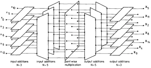
While the divide and conquer approach used in the C o o l e y - T u k e y algorithm can be understood as a 'false' mono- to multi-dimensional mapping (this will be detailed later), G o o d ' s mapping, which can be used when the factors of the transform lengths are coprime, is a true mono- to multi-dimensional mapping, thus having the advantage of not produc- ing any twiddle factor.
Its drawback, at first sight, is that it requires efficiently computable DFTs on lengths which are coprime: For example, a D F T o f length 240 will be d e c o m p o s e d as 240 = 16 • 3 • 5, and a D F T o f length 1008 will be d e c o m p o s e d in a n u m b e r of DFTs of lengths 16, 9 and 7. This method thus
requires a set of (relatively) small-length DFTs that seemed at first difficult to compute in less than N~ operations. In 1968, however, Rader showed how to map a D F T of length N, N prime, into a circular convolution of length N - 1 [43].
However, the whole material to establish the new algorithms was not ready yet, and it took Winograd's work on complexity theory, in par- ticular on the n u m b e r of multiplications required for computing polynomial products or convol- utions [55] in order to use G o o d ' s and Rader's results efficiently.
All these results were considered as curiosities when they were first published, but their combina- tion, first done by Winograd and then by Kolba and Parks [39] raised a lot of interest in that class of algorithms. Their overall organization is as follows:
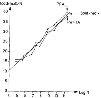
After mapping the D F T into a true multi- dimensional D F T by G o o d ' s method and using the fast convolution schemes in order to evaluate the prime length DFTs, a first algorithm makes use of the intimate structure of these convolution schemes to obtain a nesting o f the various multipli- cations. This algorithm is known as the Winograd Fourier transform algorithm (WFTA) [54], an algorithm requiring the least known number o f multiplications among practical algorithms for moderate lengths DFTs. If the nesting is not used, and the multi-dimensional D F T is performed by the r o w - c o l u m n method, the resulting algorithm is known as the prime factor algorithm (PFA) [39]
which, while using more multiplications, has less additions and a better structure than the WFTA.
From the above explanations, one can see that these two algorithms, introduced in 1976 and 1977 respectively, require more mathematics to be understood [19]. This is why it took some effort to translate the theoretical results, especially con- cerning the WFTA, into actual computer code.
It is even our opinion that what will remain mostly o f the WFTA are the theoretical results, since although a beautiful result in complexity theory, the WFTA did not meet its expectations once implemented, thus leading to a more critical
Vol. 19, No. 4, April 1990
2 6 4 P. Duhamel, M. Vetterli / A
evaluation o f what 'complexity' meant in the con- text o f real life computers [41,108, 109].
The result of this new look at complexity was an evaluation o f the n u m b e r o f additions and data transfers as well (and no longer only of multiplica- tions). Furthermore, it turned out recently that the theoretical knowledge brought by these approaches could give a new understanding o f FFTs with twiddle factors as well.
2.4. Multi-dimensional D F T s
Due to the large amount o f computations they require, the multi-dimensional DFTs as such (with c o m m o n factors in the different dimensions, which was not the case in the multi-dimensional transla- tion of a mono-dimensional problem by PFA) were also carefully considered.
The two most interesting approaches are cer- tainly the vector radix F F T (a direct approach to the multi-dimensional problem in a C o o l e y - T u k e y mood) proposed in 1975 by Rivard [91] and the polynomial transform solution o f Nussbaumer and Quandalle in 1978 [87, 88].
Both algorithms substantially reduce the com- plexity over traditional r o w - c o l u m n computa- tional schemes.
2.5. State o f the art
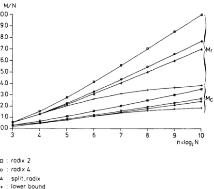
From a theoretical point o f view, the complexity issue of the discrete Fourier transform has reached a certain maturity. Note that Gauss, in his time, did not even count the number o f operations necessary in his algorithm. In particular, Winograd's work on DFTs whose lengths have coprime factors both sets lower bounds (on the number o f multiplications) and gives algorithms to achieve these [35, 55], although they are not always practical ones. Similar work was done for length-2" DFTs, showing the linear multiplicative complexity o f the algorithm [28, 35, 105] but also the lack o f practical algorithms achieving this minimum (due to the tremendous increase in the number o f additions [35]).
Signal Processing
tutorial on fast Fourier transforms
Considering implementations, the situation is of course more involved since many more parameters have to be taken into account than just the number o f operations.
Nevertheless, it seems that both the radix-4 and the split-radix algorithm are quite popular for lengths which are powers of 2, while the PFA, thanks to its better structure and easier implementation, wins over the WFTA for lengths having coprime factors.
Recently, however, new questions have come up because in software on the one hand, new pro- cessors may require different solutions (vector pro- cessors, signal processors), and on the other hand, the advent o f VLSI for hardware implementations sets new constraints (desire for simple structures, high cost o f multiplications versus additions).
3. Motivation (or: why dividing is also conquering) This section is devoted to the method that under- lies all fast algorithms for DFT, that is the 'divide and conquer' approach.
The discrete Fourier transform is basically a matrix-vector product. Calling (x0, x ~ , . . . , XN_0 x the vector o f the input samples,
(X0, X1 . . . . , XN_1) r
the vector o f transform values and W N the primi- tive N t h root o f unity (WN =e-J2~/N), the D F T can be written as
T
.x, / / 1 wN olr, , w~, , w~ ' ... ' w~-' '1
/
[x~,-d I.i w~ -' w~ ;~-" . . . w ~ -'~N-']
LI°1
x 1× x 2 : •
x 3
- 1
(1)
The direct evaluation of the matrix-vector prod- uct in (1) requires of the order of N 2 complex multiplications and additions (we assume here that all signals are complex for simplicity).
The idea o f the 'divide and conquer' approach is to map the original problem into several sub- problems in such a way that the following inequality is satisfied:
cost(subproblems) + cost(mapping)
<cost(original problem). (2) But the real power of the method is that, often, the division can be applied recursively to the sub- problems as well, thus leading to a reduction of the order o f complexity.
Specifically, let us have a careful look at the D F T transform in (3) and its relationship with the z-transform o f the squence {xn} as given in (4).
N - - 1
Xk = ~. x , W ~ , k = 0 , . . . , N - 1 , (3)
i = 0 N - - I
X ( z ) = E x,z . -' (4)
i = 0
{Xk} and {x~} form a transform pair, and it is easily seen that Xk is the evaluation of X ( z ) at point z = wTvk:
x k = X ( z ) z = w~ k. (5)
Furthermore, due to the sampled nature o f {x,}, {Xk} is periodic, and vice versa: since {Xk} is sampled, {x,} must also be periodic.
From a physical point o f view, this means that both sequences {x,} and {Xk} are repeated in- definitely with period N.
This has a number o f consequences as far as fast algorithms are concerned.
All fast algorithms are based on a divide and conquer strategy, we have seen this in Section 2.
But how shall we divide the problem (with the purpose o f conquering it)?
The most natural way is, o f course, to consider subsets o f the initial sequence, take the D F T o f these subseqnences, and reconstruct the D F T of the initial sequence from these intermediate results.
Let It, / = 0 , . . . , r - 1 be the partition of {0, 1 , . . . , N - 1 } defining the r different subsets of the input sequence. Equation (4) can now be rewritten as
N - I r - I
X ( z ) = Z x, z - i = ~, Z xi z-i, (6)
i = 0 1--0 iEl i
and, normalizing the powers of z with respect to some x0t in each subset It:
r - - 1
X ( z ) = Z z-'o, Z x,z -'÷'°'- (7)
I = 0 ielt
From the considerations above, we want the replacement of z by W ~ k in the innermost sum o f (7) to define an element o f the D F T of {xi[i ~ It}.
O f course, this will be possible only if the subset {xili ~ It}, possibly permuted, has been chosen in such a way that it has the same kind o f periodicity as the initial sequence. In what follows, we show that the three main classes o f F F T algorithms can all be casted into the form given by (7).
- - I n some cases, the second sum will also involve elements having the same periodicity, and hence will define DFTs as well. This corresponds to the case of G o o d ' s mapping: all the subsets Ij have the same number o f elements m = N / r and (rn, r ) = 1.
- - I f this is not the case, (7) will define one step o f an F F T with twiddle factors: when the subsets /l all have the same n u m b e r of elements, (7) defines one step o f a radix-r FFT.
- - I f r = 3, one o f the subsets having N / 2 elements, and the other ones having N / 4 elements, (7) is the basis of a split-radix algorithm.
Furthermore, it is already possible to show from (7) that the divide and conquer approach will always improve the efficiency of the computation.
To make this evaluation easier, let us suppose that all subsets It have the same number o f ele- ments, say N1. If N = N1 • N2, r = N2, each of the innermost sums of (7) can be computed with N 2 multiplications, which gives a total of N 2 N 2, when taking into account the requirement that the sum over i ~ It defines a DFT. The outer sum will need r - - N 2 multiplications per output point, that is N2 • N for the whole sum.
Vol. 19, No. 4. April 1990
266
Hence, the total n u m b e r of multiplications needed to compute (7) is
N2" N + N2" N~
= N 1 • N2( NI + N2) < N 2" N~
if N1, N 2 > 2 , (8)
which shows clearly that the divide and conquer approach, as given in (7), has reduced the number o f multiplications needed to compute the DFT.
O f course, when taking into account that, even if the outermost sum o f (7) is not already in the form of a DFT, it can be rearranged into a D F T plus some so-called twiddle-factors, this mapping is always even more favorable than is shown by (8), especially for small N~, /V2 (for example, the length-2 D F T is simply a sum and difference).
Obviously, if N is highly composite, the division can be applied again to the subproblems, which results in a number o f operations generally several orders of magnitude better than the direct matrix- vector product.
The important point in (2) is that two costs appear explicitly in the divide and conquer scheme: the cost o f the mapping (which can be zero when looking at the number o f operations only) and the cost o f the subproblems. Thus, different types o f divide and conquer methods attempt to find various balancing schemes between the mapping and the subproblem costs. In the radix-2 algorithm, for example, the subproblems end up being quite trivial (only sum and differen- ces), while the mapping requires twiddle factors that lead to a large n u m b e r o f multiplications. On the contrary, in the prime factor algorithm, the mapping requires no arithmetic operation (only permutations), while the small DFTs that appear as subproblems will lead to substantial costs since their lengths are coprime.
4. FFTs with twiddle factors
The divide and conquer approach reintroduced by Cooley and Tukey [25] can be used for any
Signal Processing
P. Duhamel, M. Vetterli / A tutorial on fast Fourier transforms
composite length N but has the specificity o f always introducing twiddle factors. It turns out that when the factors o f N are not coprime (for example if N = 2"), these twiddle factors cannot be avoided at all. This section will be devoted to the different algorithms in that class.
The difference between the various algorithms will consist in the fact that more or fewer o f these twiddle factors will turn out to be trivial multiplica- tions, such as 1, - 1 , j, - j .
4.1. The Cooley- Tukey mapping
Let us assume that the length o f the transform is composite: N = N~ • N2.
As we have seen in Section 3, we want to parti- tion { x i l i = O , . . . , N - l } into different subsets { x i l i s I~} in such a way that the periodicities o f the involved subsequences are compatible with the periodicity o f the input sequence, on the one hand, and allow to define DFTs o f reduced lengths on the other hand.
Hence, it is natural to consider decimated ver- sions o f the initial sequence:
I,, = {n2N, + n,},
nl = 0 , . . . , N 1 - 1 , n 2 = 0 . . . . , N 2 - 1,
which, introduced in (6) gives
N I - I N2--1
X(z)= Z Y x.2,,,,+.,z -~"~'+"°,
nl=O n2~O
(9)
(lO)
(11)
Using the fact that
W ~ rt -~" e-J2"rrNli/N = e - - J 2 ~ i / N 2 = WN2,i (12)
N 1 - 1 742-1
X(z)= Z z-", Z x.~N,+.,z-"#'.
h i = 0 n2=0
x~ = X(z)J=:w~
NI--1 N2--1
w n t k w n 2 N 1 k
= ~ " ' N ~" X n 2 N , + n , - - N "
n t = 0 n2=0
and, after normalizing with respect to the first element o f each subset,
P. Duhamel, M. Vetterli / A tutorial on fast Fourier transforms 267 (11) can be rewritten as
N I - - 1 N 2 - - 1
W ~k W ~k (13)
x~= Y ..N E x.~,,,,+,,..N2.
n 1 = 0 n 2 = O
Equation (13) is now nearly in its final form, since the right-hand sum corresponds to N1 DFTs o f length N2, which allows the reduction of arith- metic complexity to be achieved by reiterating the process. Nevertheless, the structure o f the C o o l e y - Tukey F F T is not fully given yet.
Call Yn,,k the kth output of the nlth such DFT:
N2-1
. . . . ~k (14)
Ynb k = ~., Xn2Nl+n I ~/N2 •
n 2 ~ 0
Note that in Y,,,k, k can be taken modulo N2, because
W ~ = WN~N~+k' = WN.N~ W ~ = W ~ . (15) With this notation, X k becomes
N I - - I
Y,, W n'k (16)
h i = 0
At this point, we can notice that all the X k for ks being congruent m o d u l o N2 are obtained from the same group of N~ outputs o f Y.,.k. ThUS, we express k as
k = k i N 2 + k2
kl = 0 , . . . , N l - 1 , k2 = 0 . . . N 2 - 1.
(17) Obviously, Yn,,k is equal to Y,,,k2 since k can be taken m o d u l o N2 in this case (see (12) and (15)).
Thus, we rewrite (16) as
N I - - 1
X k , N2+k2 = ~ Ynl,k2 W ~ (klNE+k2), ( 1 8 )
n 1 =0
which can be reduced, using (12), to
N t - - 1
X k , N~+k~ = Y. Yn,.k~ W"lk~W"Lk' "" N "" N 1 " (19)
n l = 0
Calling Yrnl,k2 the result o f the first multiplication (by the twiddle factors) in (19) we get
y , - V ll/-nl k2
,,,k~- • ,.,k~ ,, N • (20)
We see that the values o f XklN2+k 2 a r e obtained from N2 DFTs of length N~ applied on Ytnl,k2:
N 1 - - 1
XklN2+k2 ~. V ' ~t n l , k 2 rv N I • Ulnlkl (21)
n l = O
We recapitulate the important steps that lead to (21). First, we evaluated N~ DFTs of length N2 in (14). Then, N multiplications by the twiddle fac- tors were performed in (20). Finally, N2 DFTs o f length N1 lead to the final result (21).
A way o f looking at the change of variables performed in (9) and (17) is to say that the one- dimensional vector xi has been m a p p e d into a two-dimensional vector xn,,,: having N1 lines and
?42 columns. The computation of the D F T is then divided into N~ DFTs on the lines of the vector x ... a point by point multiplication with the twiddle factors and finally N2 DFTs on the columns o f the preceding result.
Until recently, this was the usual presentation of F F T algorithms, by the so-called 'index map- pings' [4, 23]. In fact, (9) and (17), taken together, are often referred to as the ' C o o l e y - T u k e y map- ping' or ' c o m m o n factor mapping'. However, the problem with the two-dimensional interpretation is that it does not include all algorithms (like the split-radix algorithm that will be seen later). Thus, while this interpretation helps the understanding of some o f the algorithms, it hinders the compre- hension o f others. In our presentation, we tried to enhance the role o f the periodicities of the prob- lem, which result from the initial choice of the subsets.
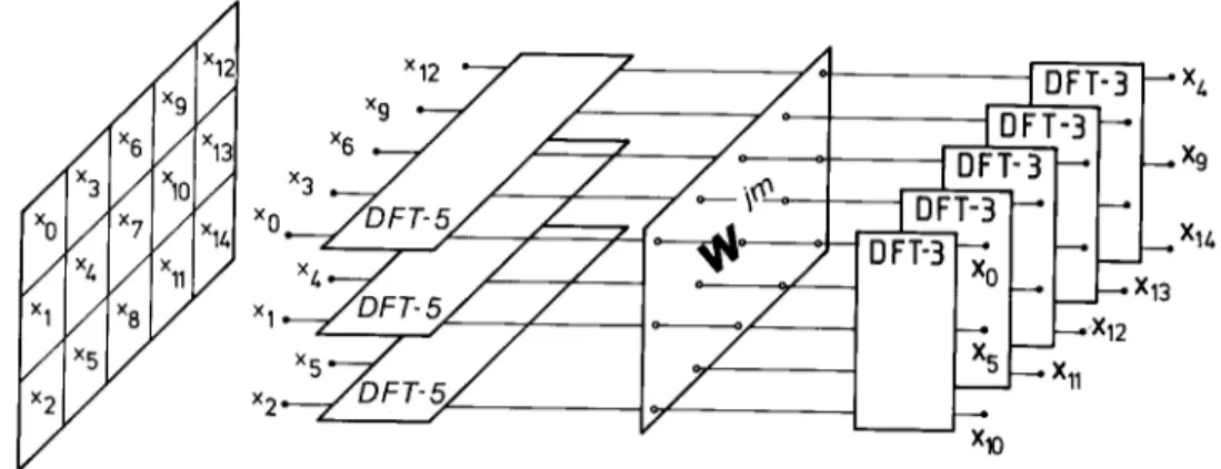
Nevertheless, we illustrate pictorially a length-15 D F T using the two-dimensional view with N1 = 3, N2 = 5 (see Fig. 1), together with the C o o l e y - T u k e y mapping in Fig. 2, to allow a precise comparison with G o o d ' s mapping that leads to the other class o f FFTs: the FFTs without twiddle factors. Note that for the case where N~ and ?42 are coprime, the G o o d ' s mapping will be more efficient as shown in the next section, and thus this example is for illustration and comparison purpose only. Because of the twiddle factors in (20), one cannot inter- change the order of DFTs once the input mapping
Vol. 19, No, 4, April 1990
268 P. Duhamel, M. Vetterli / A tutorial on fast Fourier transforms
x 6 / x3 x( x 7 / x4 x 1 x 8
lx0x3x6xgX12 Xx9
Xl/,x 4
- - Xl 0 Fig. 1. 2-D view of the length-15 Cooley-Tukey FFT.
o) N1 =3,N2=S
I Xo Xl ... X13 X1/., [
Xo X3 X6 X9 X12 X 1 X/., X 7 X10X13 X 2 X 5 X 8 Xll Xl/.,
b) Nl=5,N2 =3
X 0 X 5 Xl 0 X 1 X 6 Xll X 2 X7 X12 X 3 X 8 iX13 X/., X 9 'X14
Fig. 2. Cooley-Tukey mapping. (a) N t = 3, N 2 = 5; (b) N 1 = 5, N2=3.
has been chosen. Thus, in Fig. 2(a), one has to begin with the DFTs on the rows of the matrix.
Choosing N1 = 5, N2 = 3 would lead to the matrix o f Fig. 2(b), which is obviously different f r o m just transposing the matrix o f Fig. 2(a). This shows again that the m a p p i n g does not lead to a true two-dimensional transform (in that case, the order o f row and column would not have any importance).
Signal Processing
4.2. R a d i x - 2 and radix-4 algorithms
The algorithms suited for lengths equal to powers o f 2 (or 4) are quite p o p u l a r since sequen- ces of such lengths are frequent in signal processing (they make full use o f the addressing capabilities o f computers or DSP systems).
We assume first that N = 2". Choosing N~ = 2 and N2 = 2 " - 1 = N / 2 in (9) and (10) divides the imput sequence into the sequence of even and odd n u m b e r e d samples, which is the reason why this a p p r o a c h is called ' d e c i m a t i o n in time' (DIT). Both sequences are decimated versions, with different phases, o f the original sequence. Following (17), the output consists of N / 2 blocks of 2 values.
Actually, in this simple case, it is easy to rewrite (14), (21) exhaustively:
N/2-1
w"2k2 X k 2 = ~, X2n2 ,, N / 2
n2=0 N/2--1
k2 wn2k2 (22a)
Jr W N ~ X2n2+1 "" N / 2 ' .2=0
N/2--1
wn2k2 XN/2+k2 = ~ X2n2 - - N / 2
n2=0 N/2--1
k~ W "~k~ (22b)
-- W N Y~ X2"2+I "" N/2"
n2=O
Thus, X,, and XN/E+m are obtained by 2-point DTFs on the outputs of the l e n g t h - N / 2 D F T s o f the even and o d d - n u m b e r e d sequences, one o f which is weighted by twiddle factors. The structure
×0"
Xl ~ - N=4 -
x 2 x 3
x~ )~l DFT
N=4 X
x 6 •
x 7
W 8
• X 0 xo •
.X/. x I .-~
• X 1 x 2
• X5 x 3
• X 2 x / ,
• X6 x 5 J
.X 3 x6 J
• X 7 x 7 •
_ _ X 0
DFT
N=4 - - X 2
- - 1( 6
DFT - - x l N=4 _ _ X 3
- - X 7
division DFT multiplication DFT
info even of by of
and odd N/2 twiddle 2
numbered factors
sequences
DFT Multiplication DFT
of by of
2 lwiddle NI 2
factors
Fig. 4. D e c i m a t i o n in f r e q u e n c y r a d i x - 2 FFT.
Fig. 3. D e c i m a t i o n in t i m e r a d i x - 2 FFT.
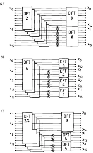
made by a sum and difference followed (or pre- ceded) by a twiddle factor is generally called a 'butterfly'. The D I T radix-2 algorithm is schemati- cally shown in Fig. 3.
Its implementation can now be done in several different ways. The most natural one is to reorder the input data such that the samples of which the D F T has to be taken lie in subsequent locations.
This results in the bit-reversed input, in-order out- put decimation in time algorithm. Another possi- bility is to selectively compute the DFTs over the input sequence (taking only the even and odd numbered samples), and perform an in-place com- putation. The output will now be in bit-reversed order. Other implementation schemes can lead to constant permutations between the stages (con- stant geometry algorithm [15]).
If we reverse the role o f N1 and N2, we get the decimation in frequency (DIF) version o f the algorithm. Inserting N1 = N/2 and N2 = 2 into (9), (10) leads to (again from (14) and (21))
N/2-1
X 2 k , = ~. W~y~(X.n,"]-XN/2+nl), ( 2 3 a ) n l = 0
N/2-1
I I rl'll k I i i t?'ll / ~.
X 2 k l + 1 = ~ W N / 2 W N t , Xni -- XN/2+nl ).
n l = O
(23b) This first step o f a D I F algorithm is represented in Fig. 5(a), while a schematic representation o f the full D I F algorithm is given in Fig. 4. The duality between division in time and division in frequency is obvious, since one can be obtained from the other by interchanging the role of {xi} and {Xk}.
Let us now consider the computational com- plexity o f the radix-2 algorithm (which is the same for the D I F and DIT version because of the duality indicated above). From (22) or (23), one sees that a D F T of length N has been replaced by two DFTs of length N/2, and this at the cost of N/2 complex multiplications as well as N complex additions.
Iterating the scheme log2 N - 1 times in order to obtain trivial transforms (of length 2) leads to the following order of magnitude of the number of operations:
OM[DFTradix.2] ~ N/2(log2 N - 1)
complex multiplications, (24a)
Vol. 19, No. 4, April 1990
270
a)
b)
c)
P. Duhamel, M. Vetterli / A tutorial on f a s t Fourier transforms
DF1
iiii'
x15"
DFT B
DFT 8
X 0
X14 Xl
• X15
ii
x 4 x15 2 Xl X13 Xl/. X3 X12 X2 X15×o DFT ' ~ DFT x°
x~ - 21/+ I ~ 8
Xlz.
x8 ~ ~ DFT I : xl
x 1 2 ~ EE Z ~ X2
| ~ /+ I • X15
Fig. 5. Comparison of various DIF algorithms for the length-16 DFT. (a) Radix-2; (b) radix-4; (c) split-radix.
OA[DFWradix_2] ~ N(log2 N - 1)
complex additions. (24b) A closer look at the twiddle factors will enable us to still reduce these numbers. For comparison purposes, we will count the number o f real operations that are required, provided that the multiplication o f a complex number x by W ~ is done using 3 real multiplications and 3 real addi- tions [12]. Furthermore, if i is a multiple o f N / 4 , no arithmetic operation is required, and only 2 real multiplications and additions are required if i is an odd multiple of N/8. Taking into account
Signal Processing
these simplifications results in the following total number o f operations [12]:
M[DFTradix.2] = 3 N / 2 log2 N - 5 N + 8, (25a) A[DFTradix_2] = 7 N / 2 log2 N - 5 N + 8.
(25b) Nevertheless, it should be noticed that these numbers are obtained by the implementation o f 4 different butterflies (1 general plus 3 special cases), which reduces the regularity o f the programs. An evaluation o f the number of real operations for other n u m b e r o f special butterflies, is given in [4], together with the number o f operations obtained with the usual 4-mult, 2-adds complex multiplica- tion algorithm.
Another case of interest appears when N is a power o f 4. Taking N1 = 4 and N 2 = N/4, (13) reduces the length-N D F T into 4 DFTs o f length N/4, about 3 N / 4 multiplications by twiddle fac- tors, and N / 4 DFTs o f length 4. The interest o f this case lies in the fact that the length-4 DFTs do not cost any multiplication (only 16 real additions).
Since there are log4 N - 1 stages and the first set of twiddle factors (corresponding to nl = 0 in (20)) is trivial, the number of complex multiplications is about
OM[OFTradix_4] ~ 3N/4(log4 N - 1). (26) Comparing (26) to (24a) shows that the number o f multiplications can be reduced with this radix-4 approach by about a factor of 3/4. Actually, a detailed operation count using the simplifications indicated above gives the following result [12]:
M[DFTradix.4]
= 9 N / 8 log2 N - 4 3 N / 1 2 + 16/3, (27a) A[DFTraeix.4]
= 2 5 N / 8 log2 N - 43N/12 + 16/3. (27b) Nevertheless, these operation counts are obtained at the cost o f using six different butterflies in the programming o f the FFT. Slight additional gains can be obtained when going to even higher radices (like 8 or 16) and using the best possible
algorithms for the small DFTs. Since programs with a regular structure are generally more com- pact, one often uses recursively the same decompo- sition at each stage, thus leading to full radix-2 or radix-4 programs, but when the length is not a power of the radix (for example 128 for a radix-4 algorithm), one can use smaller radices towards the end o f the decomposition. A length-256 D F T could use 2 stages of radix-8 decomposition, and finish with one stage of radix-4. This approach is called 'mixed-radix' approach [45] and achieves low arithmetic complexity while allowing flexible transform length (not restricted to powers o f 2, for example), at the cost of a more involved implementation.
4.3. Split-radix algorithm
As already noted in Section 2, the lowest known number of both multiplications and additions for length-2" algorithms was obtained as early as 1968 and was again achieved recently by new algorithms. Their power was to show explicitly that the improvement over fixed- or mixed-radix algorithms can be obtained by using a radix-2 and a radix-4 simultaneously on different parts o f the transform. This allowed the emergence of new compact and computationally efficient programs to compute the length-2" DFT.
Below, we will try to motivate (a posteriori!) the split-radix approach and give the derivation of the algorithm as well as its computational complexity.
When looking at the D I F radix-2 algorithm given in (23), one notices immediately that the even indexed outputs X2k, are obtained without any further multiplicative cost from the D F T of a l e n g t h - N / 2 sequence, which is not so well-done in the radix-4 algorithm for example, since relative to that l e n g t h - N / 2 sequence, the radix-4 behaves like a radix-2 algorithm. This lacks logical sense, because it is well-known that the radix-4 is better than the radix-2 approach.
From that observation, one can derive a first rule: the even samples o f a D I F decomposition
X2k should be computed separately from the other
ones, with the same algorithm (recursively) as the D F T of the original sequence (see [53] for more details).
However, as far as the odd indexed outputs X2k+~
are concerned, no general simple rule can be estab- lished, except that a radix-4 will be more efficient than a radix-2, since it allows to compute the samples through two N/4 DFTs instead of a single
N/2 D F T for a radix-2, and this at the same multiplicative cost, which will allow the cost of the recursions to grow more slowly. Tests showed that computing the odd indexed output through radices higher than 4 was inefficient.
The first recursion o f the corresponding 'split- radix' algorithm (the radix is split in two parts) is obtained by modifying (23) accordingly:
N/2-1
wT r n t k I /
X2k~= Y~ WN/ztX,,+ XN/2+,~), (28a)
n 1 = 0 N/4 1
wn~k~ W n t
X 4 k l + l ~--- ~ - - N / 4 - - N
n 1 = 0
× [ ( x . , - x N / 2 + . , )
+ j ( x n , + N / 4 -- Xn,+3N/4)], ( 2 8 b ) N/4--1
i l l n l kl I~/'3 n 1 X 4 k t + 3 = ~ vv N / 4 "" N
n 1 =0
x [(x.~ + xN/2+.~)
- j ( x , ~ + u / 4 - x,,+3N/4)]. (28c) The above approach is a D I F SRFFT, and is compared in Fig. 5 with the radix-2 and radix-4 algorithms. The corresponding D I T version, being dual, considers separately the subsets {x2i}, {x4i+~}
and {x4~+3} of the initial sequence.
Taking Io={2i}, I ~ = { 4 i + 1 } , I2={4i+3} and normalizing with respect to the first element o f the set in (7) leads to
X k =~Z.~ "~'2i~ |][zk(2i) " l - r " N " w k ~'~ X 4 i + l |'l[/rk(4i+l)-kvvN
1o I t
lll)'k(4i+ 3)-3k (29)
+ W ~ ~ x4,+3 ,, N lz
which can be explicitly decomposed in order to make the redundancy between the computation o f
Vol. 19, No. 4, April 1990