BPS Saturated String Amplitudes: K3 Elliptic Genus and Igusa Cusp Form χ

MPP–2011–77

BPS Saturated String Amplitudes:

K 3 Elliptic Genus and Igusa Cusp Form χ 10

S. Hohenegger ^a and S. Stieberger ^b

Max–Planck–Institut f¨ ur Physik Werner–Heisenberg–Institut

80805 M¨ unchen, Germany

Abstract

We study BPS saturated one–loop amplitudes in type II string theory compactified on K3 × T

²

. The classes of amplitudes we consider are only sensitive to the very basic topological data of the internal K3 manifold. As a consequence, the integrands of the former are related to the elliptic genus of K3, which can be decomposed into representations of the internal N = 4 superconformal algebra. Depending on the precise choice of external states these amplitudes capture either only the contribution of the short multiplets or the full series including intermediate multiplets. In the latter case we can define a generating functional for the whole class, which we show is given by the weight ten Igusa cusp form χ

₁₀

of Sp(4, Z ). We speculate on possible algebraic implications of our result on the BPS states of the N = 4 type II compactification.

a

shoheneg@mppmu.mpg.de

b

stephan.stieberger@mpp.mpg.de

Contents

1 Introduction 1

2 BPS Spectrum of Type II String Theory on K 3 × T

²

3

2.1 Spectrum and BPS States of Type II on K3 × T

²

. . . . 3

2.2 BPS Saturated Objects in CFT . . . . 5

3 BPS Amplitude and Short N = 4 Representations 7 3.1 BPS–Saturated Amplitude . . . . 7

3.1.1 General Setup . . . . 7

3.1.2 Bosonic Correlator . . . . 8

3.1.3 Fermionic Correlator . . . . 9

3.1.4 Complete Coupling and Holomorphic Limit . . . . 12

3.2 Holomorphic Anomaly and 1/2 BPS Contribution . . . . 13

4 Superspace Analysis and Effective Action Couplings 15 4.1 Leading On-shell 1/4 BPS Protected Coupling . . . . 16

4.2 Higher Point 1/4 BPS Protected Couplings . . . . 17

5 Intermediate Multiplets and the Elliptic Genus 18 5.1 Reducible Diagram . . . . 18

5.1.1 Singular Limit . . . . 19

5.1.2 Non-singular Limit . . . . 21

5.2 Massive External States . . . . 21

6 World–sheet Integral and Igusa Cusp Form χ

¹⁰

23 7 Conclusions 25 A N = 4 Compactifications 26 A.1 K3 Compactifications in Type II String Theory . . . . 26

A.2 Vertex Operators . . . . 27

A.2.1 Internal fields and SCFT . . . . 28

A.2.2 Zero Mass Level . . . . 28

A.2.3 First Massive Level . . . . 29

B Harmonic Superspace 30

B.1 Harmonic Coordinates . . . . 30 B.2 Linearized On-Shell Superfields . . . . 31 C World–sheet CFT and Superconformal Algebras 31 C.1 The N = 2 Superconformal Algebra . . . . 32 C.2 The N = 4 Superconformal Algebra . . . . 32 C.3 Representations . . . . 33

D Example: Orbifold Compactification 34

E World–sheet Torus Integral 35

1 Introduction

BPS–saturated amplitudes compute a very peculiar type of couplings in the effective action of string theory with extended supersymmetry. They receive contributions only from a particular class of states in the full Hilbert space, which are annihilated by a subset of the supercharges. As a consequence, these amplitudes have very interesting and unique properties. In the recent years, many examples of such couplings in string theories with N = 2 supersymmetry [1–6] as well as N = 4 supersymmetry [7–12] have been discovered. These amplitudes yield valuable information about the internal manifold of the underlying string compactification, which is encoded through a very particular dependence on the moduli. A closer study reveals, that the latter can be captured in the form of differential equations [13, 11, 5, 6], which in many cases [14, 15] allow to even compute explicit expressions for the string amplitudes.

Moreover, BPS saturated objects in string theory also teach us interesting lessons on algebraic aspects of the space of BPS states. Indeed, in [16, 17] (see also [18] for an overview) Harvey and Moore argue, that the space of BPS–states in string theory forms an algebra.

By studying certain one–loop corrections in heterotic N = 2 compactifications and relating them to the denominator formula of a (generalized) Borcherds–Kac-Moody (BKM) algebra [19] they have obtained further valuable hints on the nature of this ’algebra of BPS states’.

Similar results for the E

8

× E

8

heterotic string compactified on T

²

have recently been obtained in [20]. There it is shown, that the space of BPS–states forms a representation of a BKM–

algebra (which is constructed explicitly). The denominator formula of an extension of the

latter appears in a certain heterotic one–loop N = 4 topological string amplitude, which has previously been studied in [10, 11]. A generalization of these results to different gauge groups is studied in [21]. Since this approach is fully perturbative the topological amplitude studied in this way is only sensitive to perturbative BPS states (i.e. 1/2 BPS states after compactification down to four-dimensions).

In this work we investigate the possibility of BPS saturated amplitudes, which are also sensitive to 1/4 BPS states in a theory with N = 4 supersymmetry. To this end, we shall consider one–loop amplitudes in type II string theory compactified on K3 × T

²

and we shall particularly be interested in quantities, which have a certain ’index-like’ behaviour w.r.t.

the internal CFT living on K3, i.e. we want the amplitude to be invariant under particular deformations of the latter (see especially [22] for an analogue in N = 2). Indeed, such an object would have to be sensitive only to very basic topological data of K3 and a natural candidate in the N = 4 setup is the elliptic genus of K3 [23–25]. The latter has recently attracted a lot of interest following the observation, that it might carry an action of the Mathieu group M

₂₄

[26–29]. Its appearance in the form of a BPS saturated amplitude might therefore give additional hints about algebraic properties of the space of N = 4 BPS states.

Besides this, the elliptic genus is also the seed function for an infinite product representation of a certain weight ten Siegel modular form of Sp(4, Z ), known as the Igusa cusp form χ

10

. The latter is proposed to encode the degeneracies of (non-perturbative) dyonic 1/4 BPS- states in N = 4 string compactifications [30]. It has already been shown earlier in [31], that this infinite product representation can be related to the denominator formula of a certain rank 3 (super) BKM-algebra. This suggests that degeneracies of dyons also become related to the root multiplicities of the associated BKM–algebra. The physical role of this BKM–

algebra has been further clarified in [32] (see also [33–35]), where it has been shown, that the wall–crossing behaviour of the dyon spectrum is controlled by the hyperbolic Weyl group of this BKM–algebra.

A series of 1/4 BPS saturated one–loop amplitudes has been studied in [8]. In this

reference the (fermionic contractions of the) 2K + 4–point couplings (∂

ν

T ∂

^ν

U )

^K+1

(∂

ρ

φ∂

^ρ

φ) ¯

are computed for K ≥ 0 at the one-loop level in type II superstring theory compactified

on K 3 × T

²

. Here φ ∈ { T, U } describe the K¨ahler and complex structure moduli of the

torus T

²

. However, this set of couplings does not entail the elliptic genus of K3, but rather

another index–like object related to the torus T

²

. Indeed, the only topological information

on K3 entering these particular couplings is the Euler number. It is one of the motivations

for this work to investigate amplitudes, which encode slightly more topological information

on K3. Indeed, we propose several new BPS–saturated amplitudes, which we show to be

related to (parts of) the elliptic genus of K3. In fact, we can distinguish between two

different scenarios: In a first approach we consider a coupling of the form R

²₍₊₎

F

₍₋₎^2N

, where

R

(+)

is the self-dual part of the Riemann tensor and F

(−)

the anti-self-dual part of the field

strength tensor of one of the Kaluza-Klein vector fields stemming from the compactification

on K3 × T

²

. In particular, all these component fields are part of (massless) 1/2 BPS short multiplets in the N = 4 string effective action. We show, that this coupling can be linked to the contribution of massless short N = 4 multiplets to the elliptic genus of K3. In fact, after summing over N , we recover a particular Appell–Lerch sum, which falls into the class of mock modular forms, that have been introduced by Ramanujan and which have recently attracted a lot of attention both in mathematics and physics (see e.g. [36] for a nice overview). We also discuss the exact structure of these effective action couplings using N = 4 harmonic superspace in the supergravity frame. In order to obtain the full elliptic genus (including also the contribution of the intermediate multiplets), we have to consider amplitudes, whose external fields are part of massive multiplets. We compute those amplitudes in two distinct ways: First as a reducible limit of a 1/2 BPS amplitude (i.e. with the position of two of the external insertions colliding) and secondly directly using massive vertices. Upon introducing a coupling constant λ, we demonstrate in both ways that we can indeed define a generating functional of one–loop string amplitudes, which eventually resembles the elliptic genus of K3. We explicitly perform also the world-sheet torus integral and prove that this generating functional is given by the weight ten Igusa cuspform χ

10

of Sp(4, Z ).

This work is organized as follows: In section 2 we will review important aspects of the BPS spectrum of type IIA string theory compactified on K3 × T

²

, emphasizing important BPS-saturated index-like objects. In section 3 we will first consider a one-loop amplitude with external fields residing in short (1/2 BPS) multiplets. We will evaluate this amplitude up to the integration over the world-sheet torus and find that the integrand is related to a particular part of the elliptic genus of K 3. Indeed, by expanding the latter in terms of characters of N = 4 representations (along the lines of [37, 38, 26]) we see that the integrand is given by a particular Appell-Lerch sum, which captures the contributions from short N = 4 multiplets. We give also a superspace description of this particular class of couplings in terms of harmonic superspace in section 4. In a next step in section 5 we consider a class of amplitudes which contain massive external fields. We provide two ways of computing these amplitudes: (i) as collinear limits of 1/2 BPS amplitudes; (ii) directly by the use of massive scalar field vertices. Both methods lead to the same result, a torus integral, whose integrand is given by derivatives of the (full) elliptic genus of K3. In section 6, by introducing a coupling constant λ, we define a generating functional for this class of amplitudes. Direct evaluation of the torus integration shows that this functional is the Igusa cusp form χ

10

, which depends on λ as well as the moduli of the internal T

²

torus.

This work is accompanied by five appendices, which contain additional information about

the internal CFT of type II N = 4 compactifications as well as several computations that

we deemed too lengthy to fit into the main body of this paper.

2 BPS Spectrum of Type II String Theory on K 3 × T ²

The most basic string theories with N = 4 supersymmetry in D = 4 space–time dimensions are type IIA or type IIB compactified on K3 × T

²

or equivalently heterotic string theory compactified on a six–torus T

⁶

. In the following we shall concentrate on type IIA on K 3 × T

²

and present its spectrum.

2.1 Spectrum and BPS States of Type II on K 3 × T ²

The effective action of type II superstring theory compactified on K3 × T

²

is described by N = 4 supergravity in D = 4. The massless spectrum consists of the N = 4 supergravity multiplet coupled to 28 vector multiplets (VMs). As reviewed in appendix B.2, the latter contain a vector field A

µ

(transforming in the adjoint of the gauge group), four Weyl spinors λ

ⁱ

and six real scalars ϕ

^ij

, with ϕ

^ij

= − ϕ

^ji

, where i, j = 1, . . . , 4 are indices of the SU(4) R-symmetry group. Out of the 28 VMs only 22 are physical, while the remaining 6 act as compensating multiplets. As was explained in detail in e.g. [11], the 36 scalars of these multiplets are eliminated by imposing the D-term constraints (20 constraints) as well as gauge fixing Weyl invariance (one constraint) and local SO(6) symmetry (15 constraints).

The remaining 134 scalars

¹

from the Weyl multiplet and the remaining 22 VMs span the coset space M :

M = SU(1, 1)

U (1) ⊗ SO(22, 6, R )

SO(22, R ) × SO(6, R ) . (2.1) The first factor of (2.1) is described by the K¨ahler modulus T = T

₁

+ iT

₂

of the two–torus T

²

, while its complex structure modulus U = U

₁

+ iU

₂

, the σ–model moduli of K3, the type IIA dilaton field S and the Wilson lines on T

²

of the Ramond–Ramond (R–R) gauge fields parameterize the second factor. In type II compactification on K3 × T

²

two supercharges from the left– and right–movers each comprise the full N = 4 SUSY algebra. Therefore, half of the gauginos λ

^a

originate from the R–NS sector and the second half ˜ λ

^a

from the NS–R sector. The corresponding string world–sheet emission vertex operators of these fields are given in appendix A.2.

In type IIA the 22 gauge vectors A

^a_µ

in the VMs arise from the R–R 3–form potentials C

µij

reduced on the b

2

(K 3) = 22 two–cycles of K3 with the index a labeling the internal SCFT, cf. appendix A.2. On the other hand, the six graviphoton fields B

_µ^b

from the supergravity multiplet stem from the R–R 1–form C

µ

in D = 10, the R–R 3–form C

µ45

reduced on T

²

, the

1

Physically, in type IIA these scalars arise as follows: The σ–model of K3 has 80 and that of T

²

four

real deformations. The R–R 1–form gives rise to the two real scalars C

4

, C

5

and the R–R 3–form gives

b

3

(K3 × T

²

) = 44 scalars. Reducing the R–R 3–form down to an anti–symmetric space–time 2–tensor, which

can be dualized to a scalar, gives b

1

(K3 × T

²

) = 2 more scalars. Together with the dilaton field S we obtain

80 + 4 + 2 + 44 + 2 + 2 = 134 real scalars.

NS–NS anti–symmetric tensor B

µ4

, B

µ5

and metric g

µ4

, g

µ5

reduced along the two one–cycles of the torus T

²

.

To all these gauge fields electric and magnetic charged objects are associated. In partic- ular, the fundamental string wrapped on T

²

with winding numbers n

1

, n

2

and Kaluza–Klein (KK) momenta m

1

, m

2

is electrically charged under the gauge fields B

µ4

, B

µ5

, g

µ4

, g

µ5

with the charges n

1

, n

2

, m

1

, m

2

∈ Z , respectively. Their corresponding magnetic counter parts are described by the NS five–brane wrapped on K

3

× S

¹

and a KK monopole on S

¹

. The remain- ing charges are carried by D0, D2, D4 and D6–branes wrapped around the corresponding cycles. We refer the reader to Ref. [39] for a recent exhibition on these states.

The mass of a fundamental type II NS–NS closed string state wrapped around the torus T

²

with windings n

1

, n

2

and momenta m

1

, m

2

is given by

m

²_L

= N

L

−

¹₂

+ | P

L

|

²

+ (p

µ

)

²

,

m

²_R

= N

R

−

¹₂

+ | P

R

|

²

+ (p

µ

)

²

, (2.2) with the Narain momenta (P

L

, P

R

) ∈ Γ

^2,2

P

L

= 1

√ 2T

2

U

2

(m

1

+ m

2

U + n

1

T ¯ + n

2

T U ¯ ) ,

P

R

= 1

√ 2T

2

U

2

(m

1

+ m

2

U + n

1

T + n

2

T U ) , (2.3) corresponding to the torus T

²

. Level matching requires:

m

²_L

− m

²_R

= N

L

− N

R

+ | P

L

|

²

− | P

R

|

²

= N

L

− N

R

+ 2 (m

1

n

2

− n

1

m

2

) = 0 . (2.4) A particular interesting class of states, which will also attract our attention in the sequel, are the so–called Dabholkar–Harvey (DH) states. The latter are perturbative BPS states, which may either have left–moving N

L

or right–moving N

R

excitations:

N

R

, N

L

= 0 : m

1

n

2

− n

1

m

2

= 0 , 1/2 BPS , N

_L

= 0 : 2 (m

₁

n

₂

− n

₁

m

₂

) = N

_R

, 1/4 BPS , N

R

= 0 : 2 (n

1

m

2

− m

1

n

2

) = N

L

, 1/4 BPS .

(2.5)

Depending on the value of the duality invariant m

1

n

2

− n

1

m

2

these states represent either 1/2 or 1/4 BPS saturated string states. In the remainder of this paper we will be very interested in string theory amplitudes which only receive contributions from such states. However, before explicitly computing such amplitudes, let us first discuss such BPS saturated objects from a (world-sheet) CFT point of view.

2.2 BPS Saturated Objects in CFT

In two-dimensional theories with extended superconformal symmetry (i.e. with N ≥ 2) the

study of objects, which receive contributions only from (a subset of) the BPS states has

proven to be very fruitful both from a mathematical and physical point of view. In the sequel we generically refer to such objects as being BPS saturated. The simplest examples are (particular cases of) helicity supertraces [40] which are generically defined as

B

_n

:= 1 (2πi)

ⁿ

∂

∂z + ∂

∂ z ¯

n

Z(z, z) ¯

z=¯z=0

, for n ∈ N

_even

, (2.6)

where Z(z, z) is the following generating functional ¯ Z(z, z) := Tr ¯

RR

h

( − 1)

^{F+ ¯F}

e

^2πizJ0

e

^{−2πi¯zJ¯0}

q

^L0−24c

q ¯

^L¯0−24c¯

i

, with q := e

^2πiτ

. (2.7) Here, c is the central charge of the CFT, F + ¯ F is the total fermion number, L

0

and ¯ L

0

are the zero modes of the Virasoro generators, J

0

and ¯ J

0

the zero modes of the (left- and right-moving) U (1) R–symmetry currents and the trace is over the full Ramond sector of the theory. We note that B

n

= 0 for n odd and for n < N . In fact, for N ≤ n < 2 N the only contribution to B

n

stems from BPS representations (i.e. ’short’ or ’intermediate’

multiplets) in the trace in (2.7), while for n ≥ 2 N generic representations contribute [40].

In the case of N = 4 supersymmetry, relevant in this work, the interesting (BPS–saturated) traces are B

4

and B

6

. The object B

4

is only sensitive to 1/2 BPS representations (’short’

multiplets) while 1/4 BPS representations (’intermediate multiplets’) could be relevant

²

for B

₆

. However, a more careful analysis shows, that also B

₆

only receives contributions from 1/2 BPS representations and that the intermediate multiplets mutually cancel out. This can e.g. be immediately seen in the case of heterotic string theory compactified on T

⁶

(which is dual to type II on K3 × T

²

) [39, 42].

A different BPS saturated quantity, which is defined for any SCFT with N ≥ 2 is the elliptic genus

³

[23–25]

φ(τ, z) := Tr

_RR

h

( − 1)

^{F+ ¯F}

e

^2πizJ0

q

^L0−24c

q ¯

^L¯0−24¯c

i

, (2.8)

where the trace is taken over the Ramond-sector of the CFT. Due to the usual index type of arguments only the ground states contribute from the right moving sector and thus φ(τ, z) is a holomorphic function independent of ¯ τ . More precisely, using modularity properties of the CFT together with spectral-flow invariance one can prove [45] that the elliptic genus transforms as a weak Jacobi form [46] of index m = c/6 and weight 0.

In this work we will mainly be interested in the ellitpic genus of a CFT with target space

⁴

K3 (with central charge c = 6). In this case φ

_K3

is an universal quantity in the sense that it

2

Indices counting M2–branes in K3 × T

²

have been discussed in [41] from an M–theory perspective.

3

The elliptic genus plays an important role in the computation of anomaly cancellation terms and other exact quantities in the string effective action at one–loop [43, 44].

4

For some recent work on symmetry properties of such sigma models as well as the definition of twisted

versions of φ (so called twining genera ) in these models see [47].

does not depend on the target space moduli and is given by the following rational function of Jacobi theta functions

φ

K3

(τ, z) = 8

"

θ

2

(τ, z) θ

2

(τ, 0)

2

+

θ

3

(τ, z) θ

3

(τ, 0)

2

+

θ

4

(τ, z) θ

4

(τ, 0)

2

#

≃ 2y + 20 + 2y

⁻¹

+ q 20y

²

− 128y + 216 − 128y

⁻¹

+ 20y

⁻²

+ O (q

²

) . (2.9) In terms of the N = 4 algebra, φ

K3

is sensitive to short and intermediate representations.

Indeed, following [37, 38] (see also the more recent paper [26]) we can expand φ

K3

φ

_K3

(τ, z) = 24 ch

^N=4

h=1

4,ℓ=0

(τ, z) +

∞

X

n=0

A

_n

ch

^N=4

h=n+1 4,ℓ=1

2

(τ, z)

= 24 ch

^N=4

h=1

4,ℓ=0

(τ, z) + Σ(τ) θ

1

(τ, z)

²

η(τ)

³

, (2.10)

where we have introduced (see [48]) ch

^N=4

h,ℓ=1 2

(τ, z) := q

^h−38

θ

1

(τ, z)

²

η(τ)

³

, ch

^N=4

h=1

4,ℓ=0

(τ, z) := θ

1

(τ, z)

²

η(τ )

³

µ(τ, z) (2.11) for the elliptic genera of the intermediate and short N = 4 representations, respectively.

The coefficients A

_n

are positive integers and it is shown up to very high n in [26–29], that they can be decomposed into dimensions of irreducible representations of the Mathieu group M

₂₄

with non-negative integer multiplicities

⁵

. Furthermore, µ(τ, z) is an Appell–Lerch sum defined as

µ(τ, z) = − ie

^πiz

θ

1

(τ, z)

∞

X

n=−∞

( − 1)

ⁿ

q

^n(n+1)2

e

^2πinz

1 − q

ⁿ

e

^2πiz

, (2.12) and we also have used the weight 1/2 mock modular form Σ(τ ):

Σ(τ ) = − 8

µ τ, u =

¹₂

+ µ τ, u =

^1+τ₂

+ µ τ, u =

^τ₂

= − 2 q

⁻¹⁸

1 −

∞

X

n=1

A

n

q

ⁿ

! . (2.13)

3 BPS Amplitude and Short N = 4 Representations

In this section we consider a BPS–saturated one-loop amplitude with external legs stemming from 1/2 BPS short multiplets of type II string theory compactified on K 3 × T

²

. As we shall see, this amplitude captures only the contribution of massless short multiplets to the elliptic genus of K3. As has already been discussed in the previous section (see also [37, 38]) this contribution can be written in terms of an Appell-Lerch sum.

5

This observation, which is known in the literature under the name Mathieu moonshine, suggests the

existence of a non-trivial action of M

₂₄

on the space of BPS states that contribute to φ

K3

.

3.1 BPS–Saturated Amplitude

3.1.1 General Setup

We start out by considering the following BPS–saturated one–loop coupling in type II string theory compactified on K3 × T

²

G

N

R

(+),µνρτ σ

R

₍₊₎^µνρσ

F

(−),λτ

F

₍₋₎^λτ

N

, N ∈ N , (3.1)

with R

^µνρσ₍₊₎

the self-dual part of the four-dimensional Riemann tensor and F

₍₋₎^µν

the field strength of the Kaluza–Klein vector field stemming from the compactification on T

²

(i.e. the NS–NS graviphoton field strength tensor). We will choose all vertex operators to be inserted in the (0, 0)–ghost picture and their generic expressions can be found in appendix A.2. In order to simplify the computation, we choose fixed helicities for all fields, i.e. to be concrete we evaluate the amplitude

A

N

(p

2

, p ¯

2

, p ¯

⁽ⁱ⁾₂

, p

⁽ⁱ⁾₂

) = (3.2)

* Z

d

²

z

1

V

_R^(0,0)

(h

11

, p

2

) Z

d

²

z

2

V

_R^(0,0)

(h

¯1¯1

, p ¯

2

)

N

Y

i=1

Z

d

²

x

i

V

_F^(0,0)

(ǫ

⁽ⁱ⁾₁

, p ¯

⁽ⁱ⁾₂

) Z

d

²

y

i

V

_F^(0,0)

(ǫ

⁽ⁱ⁾_¯1

, p

⁽ⁱ⁾₂

) +

In order to resemble the coupling (3.1) we need to extract the piece proportional to the momentum structure p

²₂

p ¯

²₂

Q

N

i=1

p ¯

⁽ⁱ⁾₂

p

⁽ⁱ⁾₂

. Comparing to (A.9) and (A.10) we realize that both the bosonic as well as the fermion bilinear piece of the vertex operators will contribute.

Therefore, the whole correlator can be written in the following way:

G

^N

= Z

dζ[N ]

N

X

n=0 2N

2n

*

ψ

1

ψ

2

(z

1

) ¯ ψ

1

ψ ¯

2

(z

2

)

n

Y

i=1

ψ

1

ψ ¯

2

(x

i

) ¯ ψ

1

ψ

2

(y

i

) +

D ψ ˜

1

ψ ˜

2

(¯ z

1

) ψ ¯˜

1

ψ ¯˜

2

(¯ z

2

) E

×

*

_N

Y

j=n+1

( ¯ X

2

∂X

1

)(x

j

) (X

2

∂ X ¯

1

)(y

j

) + *

_N

Y

i=1

∂X ¯

3

(¯ x

i

) ¯ ∂X

3

(¯ y

i

) +

=

N

X

n=0 2N

2n

G

N^bos−n

G

n^ferm

. (3.3) We have introduced the shorthand notation R

dζ[N ] := R

d

²

z

_1,2

Q

^N

i=1

R d

²

x

_i

R

d

²

y

_i

for the inte- gral measure. In the following we compute the various correlators separately.

3.1.2 Bosonic Correlator

The bosonic part of the correlator (3.3) takes the form G

N^bos−n

= (P

R

)

^2N

*

_N

Y

j=n+1

Z

d

²

x

i

( ¯ X

2

∂X

1

)(x

j

) Z

d

²

y

i

(X

2

∂ X ¯

1

)(y

j

) +

, (3.4)

where we have already used that the fields ¯ ∂X

3

cannot contract with each other and therefore only contribute through their zero-modes. The correlator (3.4) can be computed in a straight- forward way using path integral methods. Indeed, following [2] we obtain:

G

_N−n^bos

= (P

R

)

^2N

τ

₂^2N−2n

∂

^2N−2n

∂w

^2N−2n

G(w)

w=0

≡ (P

R

)

^2N

τ

₂^2N−2n

"

∂

^2N−2n

∂w

^2N−2n

∞

X

g=1

w

^2g

(g!)

²

τ

₂^2g

*

_g

Y

i=1

Z

d

²

x

i

X ¯

2

∂X

1

(x

i

) Z

d

²

y

i

X

2

∂ ¯ X ¯

1

(y

i

) +#

w=0

.

The generating functional G(w) can be expressed in terms of the following normalized func- tional integral of two complex scalar fields

G(w) = R Q

2

i=1

D X

i

D X ¯

i

Exp

− S +

_τ^w₂

R

( ¯ X

2

∂X

1

+ X

2

∂ X ¯

1

) R Q

2

i=1

D X

i

D X ¯

i

Exp ( − S) =

2πiw η(τ)

³

θ

1

(w, τ )

2

e

^−2πw

2 τ2

,

(3.5) where S is the usual free-field action S = P

i=1,2 1 π

R d

²

x(∂X

i

∂ ¯ X ¯

i

+ ∂ X ¯

i

∂X ¯

i

). The evaluation of the functional integral has been performed in [2] (see also

⁶

[4]). In total we find for the bosonic part of the amplitude:

G

N^bos−n

= (P

R

)

^2N

τ

₂^2N−2n

"

∂

^2N−2n

∂w

^2N−2n

2πiw η(τ )

³

θ

1

(w, τ)

2

e

^−2πw

2 τ2

#

w=0

. (3.6)

3.1.3 Fermionic Correlator

To compute the fermionic part of the correlator (3.3) we work at a generic point in the moduli space of K3 and use the following table summarizing the charges in the SO(2) × Γ lattice (see appendix A.1 for more details):

vertex # pos. φ

1

φ

2

H

3

H φ ˜

1

φ ˜

2

H ˜

3

H ˜

graviton 1 z

1

+1 +1 0 0 +1 +1 0 0

1 z

2

− 1 − 1 0 0 − 1 − 1 0 0

vector field n x

i

+1 − 1 0 0 0 0 0 0

n y

i

− 1 +1 0 0 0 0 0 0

6

A particularly useful expansion of this expression in terms of standard Eisenstein series E

2k

(τ) can e.g.

be found in [23, 49] and is given by:

_θ^2πη_1(w,τ)^3w

= − Exp

∞

P

k=1 ζ(2k)

k

E

2k

(τ) w

^2k

.

With this information it is straightforward to write down the fermionic contribution G

n^ferm

: =

Z dζ[n]

*

ψ

₁

ψ

₂

(z

₁

) ¯ ψ

₁

ψ ¯

₂

(z

₂

)

n

Y

i=1

ψ

₁

ψ ¯

₂

(x

_i

) ¯ ψ

₁

ψ

₂

(y

_i

) +

D ψ ˜

₁

ψ ˜

₂

(¯ z

₁

) ¯˜ ψ

₁

ψ ¯˜

₂

(¯ z

₂

) E

= Z

dζ[n] X

s

F

Λ,s

z

1

− z

2

+

n

P

i=1

(x

i

− y

i

), z

1

− z

2

−

n

P

i=1

(x

i

− y

i

), 0 E

²

(z

1

, z

2

) Q

n

i,j

E

²

(x

i

, y

i

)

× X

˜ s

F ˜

Λ,˜s

(¯ z

1

− z ¯

2

, z ¯

1

− z ¯

2

, 0)

E

²

(¯ z

₁

, z ¯

₂

) , (3.7)

where we have already used that the ghost contribution has canceled a ϑ-function corre- sponding to the φ

3

-plane. Here P

s,˜s

denotes the sum over all possible spin structures, which can be explicitly performed using (A.3):

G

n^ferm

= Z

dζ [n]

F

_Λ

z

₁

− z

₂

, z

₁

− z

₂

, √ 2 P

ⁿ

i=1

(x

_i

− y

_i

) E

²

(z

1

, z

2

) Q

n

i,j

E

²

(x

i

, y

i

)

F ˜

_Λ

(¯ z

₁

− z ¯

₂

, z ¯

₁

− z ¯

₂

, 0) E

²

(¯ z

1

, z ¯

2

) . Using (A.4) together with the explicit definition of the prime forms E(z

1

, z

2

) this expression can be rewritten in the following manner

G

n^ferm

= Z

dζ[n]

Θ

Λ

√ 2 P

ⁿ

i=1

(x

i

− y

i

) Q

n

i,j

E

²

(x

i

, y

i

) . (3.8) Using the bosonization identities developed in [50] we can rewrite this expression in terms of a correlator of the internal 2-dimensional CFT with target space K3

G

n^ferm

= 4τ

2

*

_n

Y

i=1

Z

d

²

x

i

e

^√2iH

(x

i

) Z

d

²

y

i

e

^−√2iH

(y

i

) +

K3

. (3.9)

This expression is however just the 2n-th derivative of the elliptic genus of K3, i.e.

G

n^ferm

= 4τ

2

∂

²ⁿ

∂z

²ⁿ

φ

K3

(τ, z)

z=0

, (3.10)

which has been introduced in (2.8). The result can either be directly obtained by rewriting the insertions in (3.9) in terms of the neutral currents J

K3

or by direct computation of the world-sheet x

i

and y

i

integrations in (3.9). The latter are most easily tackled by working at a particular point in the K3-moduli space. In fact, we perform

⁷

the calculation in an Z

₂

7

However, the calculations can easily be generalized to other orbifold points in the K3 moduli space

along [52].

orbifold limit of K3. In this case (3.9) can be written as the following correlator of fermion bilinear insertions:

G

n^ferm

= 4τ

2

X

h,g=0,1 2

*

_n

Y

i=1

Z

d

²

x

i

ψ

4

ψ

5

(x

i

) Z

d

²

y

i

ψ ¯

4

ψ ¯

5

(y

i

) +

(h,g)

. (3.11)

Correlators of this type have already been considered in [51] by breaking them down into smaller individual contractions. Indeed, denoting the fermion one-loop propagator for a particular even spin-structure β ~ = (β

1

, β

2

) by

G

^F_β~

(x − y) := h ψ

4

(x) ¯ ψ

4

(y) i

β^~

= h ψ

5

(x) ¯ ψ

5

(y) i

β^~

= 2πη(τ)

³

θ

β1

β2

(τ, x − y) θ

1/2

1/2

(τ, x − y)θ

β1

β2

(τ, 0) , (3.12) the following equality is proven in [51] for M even and M > 2

M

Y

a=1

Z

d

²

x

a

G

^F_β~

(x

1

− x

2

) G

^F_β~

(x

2

− x

3

) . . . G

^F_β~

(x

M

− x

1

) = − (2τ

2

)

^M

(M − 1)!

∂

^M

∂z

^M

ln θ

β~

(z, τ )

z=0

= 2ζ(M )(2τ

2

)

^M

2

^2β1M

E

M

(4

^2β1

τ /2 + β

1

+ β

2

+ 1/2) − E

M

(τ )

, (3.13) where E

M

denotes the M –th Eisenstein series. For M = 2 a similar expression holds with an additional non-holomorphic shift term:

Z d

²

x

1

Z

d

²

x

2

G

^F_β~

(x

1

− x

2

)

²

= (2τ

2

)

²

∂

²

∂z

²

ln θ

β~

(z, τ )

z=0

+ π τ

2

. (3.14)

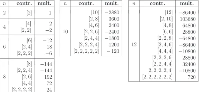
Indeed, using these expressions, we can assemble the full amplitude (3.11) by summing over all contractions with the appropriate normalization factors, which can directly be taken over from [8]. For convenience we compile the first few examples in table 1 and obtain for the fermion correlator g

_n

(τ) the final result:

g

2

(τ) = E

2

g

4

(τ) = E

4

+ E

₂²

, g

6

(τ) = − 1

12 8E

6

− 15E

4

E

2

− 5E

₂³

, g

8

(τ) = 1

72

210E

4

E

₂²

− 224E

6

E

2

+ 51E

₄²

+ 35E

₂⁴

, g

10

(τ) = 1

48

255E

₄²

E

2

+ 350E

4

E

₂³

− 560E

6

E

₂²

− 32E

6

E

4

+ 35E

₂⁵

, g

12

(τ) = 1

288

256E

₆²

− 2112E

6

E

4

E

2

− 111E

₄³

− 12320E

6

E

₂³

+ 8415E

₄²

E

₂²

+ 5775E

4

E

₂⁴

+ 385E

₂⁶

. (3.15)

n contr. mult.

2 [2] 1

4 [4]

[2, 2]

2

− 2 6

[6]

[2, 4]

[2, 2, 2]

− 12 18

− 6

8

[8]

[2, 2, 4]

[2, 6]

[4, 4]

[2, 2, 2, 2]

− 144

− 144 192 72 24

n contr. mult.

10

[10]

[2, 8]

[4, 6]

[2, 2, 6]

[2, 4, 4]

[2, 2, 2, 4]

[2, 2, 2, 2, 2]

− 2880 3600 2400

− 2400

− 1800 1200

− 120

n contr. mult.

12

[12]

[2, 10]

[4, 8]

[6, 6]

[2, 2, 8]

[2, 4, 6]

[4, 4, 4]

[2, 2, 2, 6]

[2, 2, 4, 4]

[2, 2, 2, 2, 4]

[2, 2, 2, 2, 2, 2]

− 86400 103680 64800 28800

− 64800

− 86400

− 10800 28800 32400

− 10800 720

Table 1: Overview over the cyclic contractions in the fermion correlator (3.11) for even n = 2, 4, 6, 8, 10, 12 (the correlator is identically zero for n odd) with fixed ordering of the vertices. The column ’contr.’ indicates how the original correlation function in (3.11) is decomposed into shorter correlators. Indeed, the notation [m

1

, . . . , m

k

] means that (3.11) has been broken into k correlators involving m

i

fermion pairs respectively (for more details on this notation see [8]). The third column displays the multiplicity of each decomposition.

Notice that the multiplicities of the various types of contractions, displayed in the third column, give the relative multiplicities for a given particular ordering of the vertices. Indeed, to obtain the correct result, we still need to add an overall factor of

^22nτ_(2n)!^22n(n!)2

at each step, which takes into account the appropriate combinatorial factors. Taking all contributions together, we indeed find:

G

n^ferm

= 4τ

₂²ⁿ⁺¹

∂

²ⁿ

∂z

²ⁿ

φ

K3

(τ, z)

z=0

. (3.16)

3.1.4 Complete Coupling and Holomorphic Limit

Having worked out the bosonic and fermionic part of the amplitude we are in a position to put them together and assemble the full amplitude

G

N

= 4τ

₂^2N+1

(P

_R

)

^2N

N

X

n=0 2N

2n

∂

²ⁿ

∂z

²ⁿ

∂

^2N−2n

∂w

^2N−2n

2πiw η(τ )

³

θ

1

(w, τ )

2

φ

_K3

(τ, z)e

^{−2π(w2 +z2)τ2}

z=w=0

.

(3.17)

We can explicitly perform the sum over n yielding the result G

N

= − 16π

²

τ

₂^2N+1

(P

_R

)

^2N

∂

∂z + ∂

∂w

2N

w

²

η(τ )

⁶

θ

1

(w, τ )

²

φ

_K3

(τ, z) e

^{−2π(w2 +z2)τ2}

z=w=0

. (3.18) To further simplify this expression, we introduce the new variables

u = 1

2 (z + w) , and v = 1

2 (z − w) , (3.19) such that the amplitude becomes

G

N

= − 16π

²

τ

₂^2N+1

(P

R

)

^2N

∂

^2N

∂u

^2N

(u − v)

²

η(τ )

⁶

θ

1

(u − v, τ )

²

φ

K3

(τ, u + v) e

^{−4π(u2+v2)τ2}

u=v=0

=

= − 16π

²

τ

₂^2N+1

(P

_R

)

^2N

∂

^2N

∂u

^2N

u

²

η(τ )

⁶

θ

1

(u, τ )

²

φ

_K3

(τ, u) e

^−4πu

2 τ2

u=0

. (3.20)

Note that the expression (3.20) is strongly related to the elliptic genus of K 3. In fact, in the holomorphic limit, it just corresponds to the contribution of the short multiplets with ℓ = 0. To see this, we will for the moment ignore the factor e

^−4πu

2

τ2

and moreover recall from section 2.2 that the elliptic genus can be written in the following manner

φ

K3

(τ, u) = θ

₁

(τ, u)

²

η(τ )

³

[ 24 µ(τ, z) + Σ(τ) ] , (3.21) where the object µ(τ, u) is a mock theta function, which has attracted a lot of attention recently both in mathematics and physics (see [36] and references therein for a very nice overview). With this we obtain for (the holomorphic limit of) (3.20)

G

N^hol

=



 

 

− 16π

²

τ

₂³

(P

R

)

²

η(τ)

³

h

24

_∂u^∂22

(u

²

µ(τ, u))

u=0

+ Σ(τ ) i

, N = 1

− 384π

²

τ

₂^2N+1

(P

R

)

^2N

η(τ )

³_∂u^∂NN

(u

²

µ(τ, u))

u=0

, N > 1

(3.22) Notice that the case N = 1 is somewhat different than the remaining series. We will briefly return to this point in section 4.1 where we will reinterpret this expression by calculating a slightly different (but supersymmetrically related) amplitude.

3.2 Holomorphic Anomaly and 1 / 2 BPS Contribution

To better understand the holomorphic limit, which we have discussed in the previous subsec- tion, we shall now consider the analog of the holomorphic anomaly equation [13, 1] for the coupling (3.20). To this end, let us also explicitly include the integration over the world-sheet torus as well as the Siegel–Narain theta-function for the torus compactification:

G

N

= − 16π

²

Z d

²

τ τ

2

τ

₂^2N

∂

^2N

∂u

^2N

u

²

η(τ )

⁶

θ

1

(u, τ )

²

φ

K3

(τ, u) e

^−4πu

2 τ2

u=0

× X

(PL,PR)∈Γ^2,2

(P

R

)

^2N

q

^12|PL|2

q ¯

^12|PR|2

. (3.23)

As we shall discuss at length in the next section, the integral G

^N

does not arbitrarily depend on the VM moduli, but is rather a function of just a particular harmonic-projection of the N = 4 VMs. For example (following a similar reasoning as in [1]) one would (for our conventions of Narain momenta (2.3)) expect G

N

to be independent of the modulus T . To check this we apply a (covariant) T -derivative in the following manner

D

^T

G

^N

:= 32π

²

iT

2

∂

∂T + iN 4T

2

Z d

²

τ τ

2

τ

₂^2N

P

^2N

(τ, τ ¯ ) X

(P_L,P_R)∈Γ^2,2

(P

R

)

^2N

q

^12|PL|2

q ¯

^12|PR|2

, (3.24) where we have introduced the weight (2N, 0) modular form:

P

^2N

(τ, τ) := ¯ ∂

^2N

∂u

^2N

u

²

η(τ )

⁶

θ

₁

(u, τ )

²

φ

K3

(τ, u) e

^−4πu

2 τ2

u=0

. (3.25)

We stress that P

2N

(u, τ, τ) is non-holomorphic only because of the presence of ¯ e

^−4πu2/τ2

and satisfies the recursive relation

∂

∂ τ ¯ P

2N

(τ, ¯ τ) = 2πi

τ

₂²

P

2N−2

(τ, τ ¯ ) . (3.26) Evaluating (3.24) explicitly we find

D

T

G

N

= − 16π

²

Z

d

²

τ P

2N

(τ, τ ¯ ) X

(PL,PR)

P

L

(P

R

)

^2N−1

2N − 2πτ

2

| P

R

|

²

τ

₂^2N−1

q

^12|PL|2

q ¯

^12|PR|2

= − 16π

²

Z

d

²

τ P

^2N

(τ, τ ¯ ) ∂

∂ τ ¯ X

(P_L,P_R)

P

L

(P

R

)

^2N−1

τ

₂^2N

q

^12|PL|2

q ¯

^12|PR|2

. (3.27) Performing a partial integration in ¯ τ does not give rise to a bounday contribution for N > 1.

Hence by using (3.26) we find D

T

G

N

= − 32π

³

i

Z d

²

τ τ

2

τ

₂^2N−1

P

2N−2

(τ, τ ¯ ) X

(PL,PR)

P

_L

(P

_R

)

^2N−1

q

^12|PL|2

q ¯

^12|PR|2

= 32π

²

U

₂

∂

∂ U ¯ + i(N − 1) 4U

2

Z d

²

τ τ

2

τ

₂^2N−2

P

2N−2

(τ, τ ¯ ) X

(PL,PR)

(P

_R

)

^2N−2

q

^12|PL|2

q ¯

^12|PR|2

=: 32π

²

D

U^¯

G

^N−1

, (3.28)

where we have introduced the covariant derivative with respect to ¯ U. To summarize, we have found the following recursive relation

D

T

G

N

= 32π

²

D

U^¯

G

N−1

, (3.29)

where the right hand side depends on the same G , however, with reduced index. Following

the same spirit as [1], we therefore call this contribution ’anomalous’. In the next section

we discuss its origin from an effective action point of view. However, here we notice that from the point of view of the amplitude, the anomaly is due to the e

^−4πu2/τ2

factor in the generating functional (3.25). Thus taking the holomorphic limit (as we have considered in the previous subsection) removes the anomaly and provides the ’purely topological’ coupling, which in this case corresponds to the 1/2 BPS contribution of short multiplets to the elliptic genus of K3.

4 Superspace Analysis and Effective Action Couplings

Before continuing, we investigate the amplitudes discussed in the previous section from the point of view of the effective action to understand their BPS structure. This is best il- luminated by formulating these couplings in superspace, which is suitable for manifestly displaying invariance under supersymmetry. Four dimensional theories with N = 4 super- symmetry have 16 supercharges and can therefore be best described in terms of a (4 | 16) dimensional superspace. Instead of using the standard R

^4|16

, we use harmonic superspace, which will turn out to be better suited for the description of our couplings (for a review of the relevant conventions and notation see appendix B).

The spectrum of type II string theory in N = 4 compactifications contains two types of BPS states: 1/2 and 1/4 BPS states, which group themselves in short and intermediate multiplets, respectively. They are subject to particular analyticity properties such that, roughly speaking, short multiplets depend only on half of the superspace coordinates. It turns out, that the couplings discussed in the previous section can be entirely described using short multiplets, which we have reviewed for the reader’s convenience in appendix B.2.

Before discussing the actual couplings we should also note that for the sake of manifest SO(6, 22) covariance, we will formulate all couplings in the ’supergravity frame’. Indeed, as already discussed in section 2.1, in N = 4 supergravity, the SO(6, 22) symmetry is linearized by introducing six additional compensator VMs (see [11, 12] for a more detailed discussion).

In order to reduce to only physical fields, there are two possibilities: Either the gauge fields

of the compensating multiplets are expressed as functions of the graviphotons which sit

inside the supergravity multiplet (’superstring basis’) or the relation is inverted and the

graviphotons are identified with the gauge fields of the compensating multiplets; in this

case, the vector bosons of the supergravity multiplet are expressed as functions of all VM

gauge fields (’supergravity basis’). While for explicit amplitude computations in superstring

theory, the former basis is relevant, in this section, to display manifest SO(6, 22) invariance,

we stick to the latter frame.

4.1 Leading On-shell 1 / 4 BPS Protected Coupling

Couplings involving 1/2 BPS short multiplets (Weyl and VMs) have already been discussed earlier in [10, 11]. For concreteness, here we will start out by considering a particular harmonic projection of the VM (B.8) (see also [53]), e.g.

Y

_A¹²

= Y

_A¹²

(z, θ

3

, θ

4

, θ ¯

¹

, θ ¯

²

, u) , with z

^αβ˙

= x

µ

(σ

^µ

)

^αβ˙

+ i

θ

₃^α

θ ¯

³_β˙

+ θ

₄^α

θ ¯

⁴_β˙

− θ

₁^α

θ ¯

¹_β˙

− θ

₂^α

θ ¯

²_β˙

, (4.1) where we have also added an index of the SO(6, 22) VM gauge group. This multiplet satisfies the analyticity properties

D

¹_α

Y

_A¹²

= D

_α²

Y

_A¹²

= ¯ D

^α₃^˙

Y

_A¹²

= ¯ D

^α₄^˙

Y

_A¹²

= 0 . (4.2) Thus, this multiplet can be consistently coupled to the Weyl multiplet in the following form

S = Z

d

⁴

x Z

du Z

d

²

θ

1

Z d

²

θ

2

Z d

²

θ

3

Z d

²

θ

4

Z d

²

θ ¯

¹

Z

d

²

θ ¯

²

G (W, Y

_A¹²

, u)

= Z

d

⁴

x Z

du Z

d

²

θ

3

Z d

²

θ

4

Z d

²

θ ¯

¹

Z

d

²

θ ¯

²

(D

¹

· D

¹

)(D

²

· D

²

)

G (W, Y

_A¹²

, u)

, (4.3) for some coupling function G depending also on the Weyl multiplet. This expression is an integral over 12 Grassmann coordinates and for the purpose of calculating explicit string theory amplitudes we are interested in the component expansion. Indeed, the four spinor derivatives we have explicitly written out can only hit the Weyl multiplets in the above coupling. Performing also the Grassmann integrals, we will find among others the following term at the component level

S = Z

d

⁴

x Z

du R

^(+),µνρτ

R

⁽⁺⁾_µνρτ

F

₍₋₎^A

· F

₍₋₎^B

+ F

_(−),λσ^A

λ ¯

¹_B

σ

^λσ

λ ¯

²_C

∂

∂ϕ

¹²_C

G

AB

(Φ, ϕ

¹²_A

, u) , (4.4) where we have introduced the shorthand notation

G

^AB

(Φ, ϕ

¹²_A

, u) = ∂

⁴

G (W, Y

_A¹²

, u)

∂W

²

∂Y

_A¹²

∂Y

_B¹²

θ=0

. (4.5)

The second term in the square brackets of (4.4) has just been added to show that there are also further component couplings leading to the same G

AB

. Indeed, in order to check this, we have computed the coupling

G ˜

A1A2A3

R

⁽⁺⁾_µνρτ

R

^(+),µνρτ

F

_λσ^(−),A1

λ ¯

^A₁²

σ ¯

^λσ

λ ¯

^A₂³

, (4.6)

where λ

_1,2

denote T-modulini (i.e. superpartners of the Kaluza-Klein vector fields) and F

⁽⁻⁾

is the field strength of a Kaluza-Klein vector field. Through a straight-forward computation one can show

G ˜

A1A2A3

= D

¹²A2

G

A1A3

, with G

A1A3

= Z

M

Z

d

²

w J

K3

V ˆ

A1

(w) Z

d

²

y J

K3

V ˆ

A3

(y)

+ C ,

where C is an arbitrary function which is independent of the (massless) VM moduli ϕ

¹²_A

which we will drop in the following. Notice that this is exactly the relation we have anticipated based on the superspace coupling (4.4). Choosing now a setup in which the ˆ V

A1,A3

only contribute the bosonic zero modes on the T

²

and dropping a constant tensor which takes care of the SO(n)-structure, we can rewrite this expression as:

G ∼ Tr

RR

h

( − 1)

^{F+ ¯F}

(J

0

)

²

q

^L0−14

q ¯

^L¯0−14

i

(P

R

)

²

. (4.7)

Combining this result with its conjugate, we obtain G + ¯ G ∼ Tr

RR

n ( − 1)

^{F+ ¯F}

(J

0

P

R

)

²

+ ( ¯ J

0

P

L

)

²

q

^L0−14

q ¯

^L¯0−14

o

= − 1 4π

²

∂

∂z + ∂

∂ z ¯

2

Tr

RR

h ( − 1)

^{F+ ¯F}

e

^2πizJ0PR

e

^{−2πi¯zJ¯0PL}

q

^L0−14

q ¯

^L¯0−14

i

z=¯z=0

= − 1 4π

²

∂

∂z + ∂

∂ z ¯

2

Z (zP

R

, zP ¯

L

)

z=¯z=0

, (4.8)

where Z(z, z) is the generating functional of the helicity supertraces as defined in (2.7). ¯ Expression (4.8) resembles very closely the definition (2.6) of the helicity supertrace B

₆

, which is indeed an index of the 1/2 BPS short multiplets only.

4.2 Higher Point 1 / 4 BPS Protected Couplings

The strategy in finding superspace couplings also for higher N is to consider a particular superdescendant of the VM

Υ

^µν_A

:= (D

³

σ

^µν

D

⁴

)Y

_A¹²

, (4.9) whose lowest component is indeed F

(−),A

. With this we can then consider the extended coupling

S

N

= Z

d

⁴

x Z

du Z

d

²

θ

3,4

Z

d

²

θ ¯

^1,2

(D

¹

· D

¹

)(D

²

· D

²

)

"

_N−1

Y

i=1

(Υ

Ai

· Υ

Bi

) G

^AiBi

(W, Y

_A¹²

, u)

# . (4.10) As before, evaluating all spinor derivatives and performing explicitly all the Grassmann integrations, we find (among others) the following term at the component level

S

N

= Z

d

⁴

x Z

du R

^(+),µνρτ

R

⁽⁺⁾_µνρτ

N

Y

i=1

F

₍^A₋₎

· F

₍^B₋₎

G

A1...ANB1...BN

(Φ, ϕ

¹²_A

, u) + . . . , (4.11) where we have introduced the coupling functions

G

^A1...ANB1...BN

(Φ, ϕ

¹²_A

, u) = ∂

⁴

G

_A

2...ANB2...BN

(W, Y

_A¹²

, u)

∂W

²

∂Y

_A¹²₁

∂Y

_B¹²₁

θ=0

, (4.12)

which is indeed exactly the type of coupling considered in (3.1). We can see that this coupling just depends on the particular projection ϕ

¹²

of the moduli. This would entail that i.e. derivatives with respect to, say ϕ

³⁴

should vanish. Translated into the language of the previous section, this would suggest that that G

N

is independent of T . However, as we have seen in Section 3.2, this is only correct up to an anomaly. As discussed in e.g. [1] the latter comes about due to the presence of non-analytic terms in the effective action, which (through integrating out auxiliary fields) lead to non-analytic dependencies of the higher derivative couplings. Indeed, as we had seen in Section 3.1.4, in the holomorphic limit of the amplitude (in which the anomaly is avoided) only short multiplets of the elliptic genus contribute, which is consistent with the 1/2 BPS nature of the couplings discussed here. The full string amplitude, however, restores holomorphicity of the integrand G

^N

(at the cost of modularity) thereby introducing the anomaly as discussed above.

5 Intermediate Multiplets and the Elliptic Genus

For N ≥ 1 the amplitude from the previous section receives contributions only from the short multiplets, which contribute to the elliptic genus of K3. However, the contribution of intermediate multiplets has dropped from the final expression. We want to stress, that the amplitudes considered so far, only involve external states from short (i.e. 1/2 BPS) mul- tiplets. Qualitatively different results should be expected for amplitudes involving external states from intermediate or long multiplets. In the following we shall compute these types of amplitudes in two different ways: First we shall consider reducible diagrams, i.e. amplitudes with two of the external vertices colliding. Since in the internal channels all kinds of fields are propagating, we will indeed find the elliptic genus of K3 in a very particular limit. In order to back up our computation, we will also directly compute these diagrams with massive external legs and show that the two results are in fact identical.

5.1 Reducible Diagram

Our first method of uncovering the elliptic genus of K3 will be to consider reducible diagrams.

By this we have in mind diagrams of the type depicted in figure 1, where two of the external

legs collide and form an intermediate channel. In this channel all kinds of fields, which are

allowed by the selection rules, propagate, cf. the right hand side of figure 1. By carefully

adjusting the way in which the external legs collide, we will see that it is possible to extract

the elliptic genus of K3. In fact, we will consider two distinct cases, which differ in whether

the limit in which the insertion points of two external vertices coincide is singular (and thus

needs some proper regularization), or happens to be finite.