Interest Rate Policy and the Price Puzzle in a Quantitative Business Cycle Model

IHS Economics Series Working Paper 95

February 2001

Interest Rate Policy and the Price Puzzle in a Quantitative Business Cycle Model

Andreas Schabert

Impressum Author(s):

Andreas Schabert Title:

Interest Rate Policy and the Price Puzzle in a Quantitative Business Cycle Model ISSN: Unspecified

2001 Institut für Höhere Studien - Institute for Advanced Studies (IHS) Josefstädter Straße 39, A-1080 Wien

E-Mail: o ce@ihs.ac.atffi Web: ww w .ihs.ac. a t

All IHS Working Papers are available online: http://irihs. ihs. ac.at/view/ihs_series/

This paper is available for download without charge at:

https://irihs.ihs.ac.at/id/eprint/1323/

Interest Rate Policy and the Price Puzzle in a Quantitative Business Cycle Model

Andreas Schabert

95

Reihe Ökonomie

Economics Series

95 Reihe Ökonomie Economics Series

Interest Rate Policy and the Price Puzzle in a Quantitative Business Cycle Model

Andreas Schabert February 2001

Institut für Höhere Studien (IHS), Wien

Institute for Advanced Studies, Vienna

Contact:

Andreas Schabert Department of Economics University of Cologne D-50923 Cologne, GERMANY (: +49/221/470-4532 fax: +49/221/470-5077

email: schabert@wiso-r10.wiso.uni-koeln.de

Founded in 1963 by two prominent Austrians living in exile – the sociologist Paul F. Lazarsfeld and the economist Oskar Morgenstern – with the financial support from the Ford Foundation, the Austrian Federal Ministry of Education and the City of Vienna, the Institute for Advanced Studies (IHS) is the first institution for postgraduate education and research in economics and the social sciences in Austria. The Economics Series presents research done at the Department of Economics and Finance and aims to share “work in progress” in a timely way before formal publication. As usual, authors bear full responsibility for the content of their contributions.

Das Institut für Höhere Studien (IHS) wurde im Jahr 1963 von zwei prominenten Exilösterreichern – dem Soziologen Paul F. Lazarsfeld und dem Ökonomen Oskar Morgenstern – mit Hilfe der Ford- Stiftung, des Österreichischen Bundesministeriums für Unterricht und der Stadt Wien gegründet und ist somit die erste nachuniversitäre Lehr- und Forschungsstätte für die Sozial- und Wirtschafts- wissenschaften in Österreich. Die Reihe Ökonomie bietet Einblick in die Forschungsarbeit der Abteilung für Ökonomie und Finanzwirtschaft und verfolgt das Ziel, abteilungsinterne Diskussionsbeiträge einer breiteren fachinternen Öffentlichkeit zugänglich zu machen. Die inhaltliche Verantwortung für die veröffentlichten Beiträge liegt bei den Autoren und Autorinnen.

Abstract

In the empirical literature, monetary policy shocks are commonly measured as an innovation to a short-term nominal interest rate. In contrast, the majority of monetary business cycle models treats a broad monetary aggregate as the central bank’s policy measure. We try overcome this disparity and present a business cycle model which allows to examine the effects of innovations to a non-contingent nominal interest rate rule. To obtain unique rational expectations equilibria we assume that changes in money supply are brought about open market operations. In addition to working capital, we consider staggered prices which enables real marginal costs to vary. Consistent with the empirical findings of Barth and Ramey (2000), the model predicts that real marginal cost and inflation rise in response to positive interest rate innovations. The mechanism corresponds to their ‘Cost Channel of Monetary Transmission’ and replicates typical monetary VAR results, including the puzzling behavior of prices.

Keywords

Monetary transmission, interest rate shocks, open market operations, price puzzle

JEL Classifications

E5, E3, E63

Contents

1. Introduction 1

2. The Model 3

2.1 Households ... 4

2.2 Production... 5

2.3 Fiscal and Monetary Policy ... 7

2.4 Financial Intermediation ... 9

2.5 Rational Expectation Equilibrium ... 9

2.6 Model Parametrization ... 9

3. Quantitative Properties 10

3.2 Real Marginal Cost and Inflation ... 13

4. Conclusion 15

Appendix 17

References 20

1 Introduction

What happens when an unanticipated rise in the nominal interest rate, which is commonly labeled a contractionary monetary policy shock, hits the economy? On the one hand, there is a large empirical literature presenting estimated vector autoregressive (VAR) models trying to reveal monetary policy e®ects.¹ In most of these studies monetary policy shocks are identi¯ed with innovations to the federal funds rate by imposing restrictions derived from macroeconomic theory. On the other hand, in modern monetary business cycle theory researchers develop quantitative dynamic general equilibrium models in order to study the transmission mechanism of monetary policy.² The majority of the studies, which focus on the responses to monetary policy shocks, assume that the central bank controls the growth rate of a broad monetary aggregate.

The di®erence between these two monetary policy measures becomes apparent with the so-called liquidity puzzle and the price puzzle. Monetary policy should lead to a negative correlation between nominal interest rates and monetary aggregates, i.e., the liquidity e®ect. While the liquidity e®ect can be observed in the impulse responses to federal funds rate VAR innovations, monetary business cycle models were initially unable to replicate this negative correlation. In order to eliminate this de¯ciency, models with

¯nancial market trading frictions, i.e., limited participation, were developed.³ In contrast, the price puzzle, which was raised by Sims (1992), is entirely an empirical phenomenon, or to be more pronounced, an empirical anomaly. What is meant by the price puzzle, is the protracted rise in the price level in response to a monetary contraction which is found in numerous VARs studies. The view that this ¯nding should be an anomaly is supported by practically the entire monetary theory. As a solution to this puzzle, a sensitive price index is often introduced into VARs which adds to the information set of the monetary policy reaction function. By applying such an identi¯cation scheme for monetary policy shocks, Sims (1992) showed that the price anomaly can be reduced, though it can not completely be removed in VARs.⁴ As a strategy for an appropriate selection between competing identi¯cation schemes Christiano et al. (1999) advocated to

"eliminate a policy shock measure if it implies a set of impulse response functions that is inconsistent with every element in the set of monetary models that we wish to discriminate between. This is equivalent to announcing that if none of the models that we are interested in can account for the qualitative features of a set of impulse response functions, we reject the corresponding identi¯cation assumption, not the entire set of models." (p. 70)

The purpose of the paper is to take this approach literally. For this, we understand it as a prerequisite to consider a measure for monetary policy shocks in a business cycle model which corresponds to the shock measure in VARs, namely, innovations to a short- run nominal interest rate. This assumption is clearly not new in the monetary business

1See Bernanke and Mihov (1998), and Christiano et al. (1999) for the presentation of VAR estimates using di®erent approaches and for summarizing the current state of the literature.

2Examples are Yun (1996), Chari et al. (1996), Christiano et al. (1997), Bergin and Feenstra (1998), Jeanne (1998), or Huang and Liu (1999) to name but a few.

3See, e.g., Lucas (1990), Fuerst (1992), and Christiano and Eichenbaum (1992).

4Respective point estimates reveal that a small initial rise of the GDP de°ator often remains even in the presence of a sensitive price index (see, e.g., Uhlig, 1999, and Christiano et al., 1996, 1999). See also Hanson's (2000) results which cast severe doubt on this price puzzle 'solution'.

cycle literature. Recently, several authors apply interest rate rules and in a few cases they identify monetary policy shocks with innovations to these rules.⁵ These studies are predominantly meant to study the business cycle behavior when the central bank employs a contingent monetary policy rule, such as the Taylor-Rule.⁶ Though, contingent interest rate rules are evidently more realistic, we apply a non-contingent interest rate rule in order to allow for an analysis of the genuine transmission mechanism of pure interest rate shocks.

The questions we try to help answering could be articulated as follows: Is the price puzzle, which does not completely disappear in the impulse response functions of many VARs, really an empirical anomaly? Or, should prices actually rise when ¯rms' optimal price setting is directly a®ected by rising interest rates, e.g, via interest payments on loans? To give a preview, our ¯ndings indicate that the asymmetry between the policy measure in empirical and theoretical studies is primarily responsible for puzzling results in monetary policy analysis.

The model in this paper is mainly motivated by a recent paper of Barth and Ramey (2000), titled: "The Cost Channel of Monetary Transmission". By using industrial-level data, they ¯nd that many industries exhibit rising prices in response to a rise in the nominal interest rate as the latter increases the cost of external ¯nance. Based on their empirical ¯ndings and a partial equilibrium analysis, they presume that both a supply channel (working capital) and a demand channel (price stickiness) a®ect the transmission of monetary policy shocks. On the one hand, output should decline in response to a rise in the nominal interest rate due to both of these channels. On the other hand, these channels predict di®erent reactions of real marginal costs and, hence, opposing price responses. According to the demand channel, a monetary contraction induces a decline in aggregate demand and in the price level. As an opposite impulse, the positive innovation in the nominal interest rate tends to increase the interest payments on loans which are demanded for paying the wage bill in advance, i.e., for working capital. Therefore, the in°ation reaction is unclear and depends on the impact of both channels on the real marginal cost of price setting ¯rms. Consequently, Barth and Ramey (2000) point to the still unanswered question of how monetary policy works in general equilibrium. This is where this study proceeds.

The model is fairly standard in the sense that it combines commonly used ingredients for building a monetary business cycle model.⁷ As already noted we depart from using money growth as the exogenous policy variable and we presume that the central bank controls the nominal interest rate. We apply a non-contingent interest rate policy and identify monetary policy shocks with innovations to a pure interest rate rule. Aditionally, we assume that the central bank accomodates money demand via open market operation.

We adopt this assumption, as most central banks in industrialzed countries conduct mon- etary policy in terms of directives for a short-term nominal interest rate together with accompanying open market operations. By speci¯ng the monetary and ¯scal regime in

5Examples are Clarida, Gali, and Gertler (1997), Rotemberg and Woodford (1998), McCallum (1999), McGratten (1999), or Casares and McCallum (2000).

6In a few studies interest rate rules are considered for the analysis of agency costs e®ects on the monetary transmission mechanism (see Bernanke et al., 1999, and Carlstrom and Fuerst, 2000).

7It is closely related to the model in Christiano et al.'s (1997) comparative analysis of sticky price and limited participation models.

2

this manner we obtain unique rational expectations equilibria.⁸ Along with Barth and Ramey (2000), we further assume that two transmission channels, i.e., price stickiness and working capital, are jointly at work. Applying Calvo's (1983) speci¯cation of price staggering, in°ation evolves along with a simple forward looking 'New Keynesian Phillips Curve'.

We computed the impulse response functions of the calibrated model for di®erent degrees of price stickiness. Here, we ¯nd that the impulse responses to a contractionary monetary policy shock are consistent with typical VAR results as, e.g., documented in Christiano et al. (1999). This includes that in our model in°ation rises in response to a positive nominal interest rate innovation. In accordance with the 'Cost Channel of Monetary Transmission', it is the rise in real marginal costs induced by the increased cost of loans which causes the ¯rms to raise their prices. However, the rise in the in°ation rate should be considered in the general equilibrium framework. Coincident with a real contraction, we ¯nd that the real return on capital declines. This implies that, ¯rst, the real return on bonds must also decrease to meet the arbitrage-free condition and, second, it requires that the in°ation rate rises in order to satisfy the Fisher equation. In summary, the model generally replicates empirical e®ects of an interest rate innovation. Particularly, the rise in the in°ation rate corresponds to the 'puzzling' price response in various VAR studies. As a consequence we suggest to avoid the term 'monetary contraction' when a positive interest rate innovation is meant. Our results imply that it might be necessary to improve this widespread identi¯cation scheme for monetary policy actions in order to avoid puzzling price responses in an otherwise standard business cycle model and in empirical analyses. But this issue is clearly beyond the scope of this exercise.

In the subsequent section we describe the model and it's parametrization. In section 3 we discuss the transmission mechanism and present the model's responses to an interest rate shock. Section 4 concludes.

2 The Model

In this section we present an economic environment based on the model in Christiano et al. (1997). Our speci¯cation mainly departs with respect to two assumptions. First, the monetary authority controls the nominal interest rate instead of the money growth rate.

Second, bonds are introduced together with an explicit speci¯cation of ¯scal policy. We agree to the notion of Barth and Ramey (2000) and consider that both a supply channel (working capital) and a demand channel (price stickiness) which are jointly at work.⁹

The economy consists of a government and numerous agents of three di®erent types:

households, ¯rms, and intermediaries. Money demand is induced by a cash-in-advance constraint. Substantial real e®ects of changes in monetary variables are due to staggered prices and intraperiod loans which are necessary for production. In contrast to many re- cent business cycle analyses which employ a contingent policy rule, we specify monetary policy as an non-contigent nominal interest rate rule. Accordingly, monetary policy shocks

8Woodford (1994) shows that such a combination of monetary and ¯scal policy can avoid the occurence of real indeterminacy in a cash-in-advence economy.

9Christiano et al. (1997) additionally impose that households determine the amount of deposits prior to the shock ('limited participation') to obtain a negative correlation between money growth and nominal interest rates, i.e., the liquidity e®ect.

are identi¯ed with innovations to an univariate nominal interest rate rule and money is en- dogenously supplied by the monetary authority. The government issues one-period bonds and the monetary authority accommodates money demand by an exchange of government bonds with cash in open market operations. We were guided by the ¯ndings of Woodford (1994) and adopt this kind of monetary and ¯scal policy in order to avoid real indeter- minacy which usually arises when an interest rate rule without any nominal anchor is applied.¹⁰

2.1. Households

Throughout the paper, nominal variables are denoted by upper-case letters, while real variables are denoted by lower-case letters. The typical household is in¯nitely lived, with preferences given by the expected value of a discounted stream of instantaneous utility u(:) :

E₀

"₁ X

t=0

¯^tu(ct;1¡l_t)

#

; with ¯ 2(0;1); (1)

where E₀ is the expectation operator conditional on the time 0 information set and ¯ is the discount factor. Throughout we assume that instantaneous utilityu(:) depends on a Cobb-Douglas bundle of consumptioncand leisure 1¡l, and is characterized by constant relative risk aversion (CRRA):

u(ct;1¡l_t) = [c^°_t(1¡l_t)^1¡°]^1¡¾¡1

1¡¾ ; with° 2(0;1): (2)

At the beginning of periodt;the representative household owns the entire stock of money Mt in the economy. It must decide how much of this cash holdings to keep for contempora- neous consumption and investment expenditures and how much to deposit at the ¯nancial intermediary. LetD_tdenote the amount of these deposits which will earn a nominal return of it. The rest Mt¡Dt is allocated to purchases of consumption and investment goods.

We assume that both goods must be completely ¯nanced with non-deposited cash as well as current labor income:

P_t(ct+e_t)·M_t¡D_t+P_tw_tl_t; (3) where P and w denote the aggregate price level and the real wage, respectively. The cash-in-advance constraint in (3) implies that there are no credit goods in the economy.

The household receives dividends -^f_i and the rental rate r on physical capital k as addi- tional °ows from monopolistically competitive ¯rms indexed byi2(0;1). In addition they receive dividends -^b as well as interest payments on deposits i_tD_t from ¯nancial interme- diaries. In periodtthe household chooses consumptionP_tc_t and investment expenditures Ptet, nominal money holdings Mt+1 and nominal riskless one-period pure discount bond holdings (1 +it+1)^¡1B_t+1.¹¹ Hence, cash and labor income left over from the goods market

10See Kerr and King (1996) for a discussion of the conditions for real determinacy in Keynesian models with rational expectations and interest rate rules.

11Note that there is no non-negativity restriction on the level of the household's bond holdings.

4

are carried over into the next period for money and bond holdings:

M_t+1+ (1 +i_t+1)^¡1B_t+1 (4)

=Ptrtkt+ (1 +it)Dt+Bt+ (Mt¡Dt¡Pt(ct+et¡wtlt)) + Z 1

0 -^f_itdi+ -^b_t: The household maximizes (1) sub ject to its cash-in-advance constraint (3), its budget constraint (4), and the following condition for the accumulation of physical capital:

kt+1= © µe_t

k_t

¶

kt+ (1¡±)kt; (5)

where ± denotes the depreciation rate of capital and ©(:) an increasing and concave ad- justment cost function.¹² Accordingly, investment expenditures e yield a gross output of new capital goods © (e=k)k:The inclusion of adjustment costs permits to analyze the cyclical behavior of the priceqof physical capital.¹³ The household's ¯rst order conditions for consumption, labor supply, deposit holdings, investment expenditures and for physical capital are given by

¸_t=°[c^°_t(1¡l_t)^1¡°]^1¡¾

ct(1 +it) ; (6)

w_t¸_t= (1¡°)[c^°_t(1¡l_t)^1¡°]^1¡¾

(1¡lt)(1 +it) ; (7)

¸_t

¯ =E_t

·

¸_t+11 +i_t+1

¼_t+1

¸

; (8)

q_t= (1 +i_t)©⁰ µe_t

k_t

¶_¡1

; (9)

q_t

¯ =E_t

·¸_t+1

¸_t µ

r_t+1+q_t+1 µ

© µe_t+1

k_t+1

¶

¡©⁰e_t+1

k_t+1 + (1¡±)

¶¶¸

; (10)

where ¸ and ¼ denote the Lagrange multiplier for the budget constraint and the gross in°ation rate, respectively. Furthermore, in an optimum the cash-in-advance constraint (3) holds with equality for i >0. Regarding the household's assets, the optimal choices must also satisfy the following transversality conditions:

tlim!1¯^tu_ctx_t = 0; for x=k; m; b. (11) 2.2. Production

The ¯nal good, which is consumed and invested in the stock of physical capital, is an aggregate of a continuum of di®erentiated goods produced by monopolistically competitive

¯rms indexed withi2 (0;1) . The aggregator of di®erentiated goods is de¯ned as follows:

yt =

·Z 1 0 y

(²¡1)

²

it di

¸_²¡1^²

; with² >1; (12)

12Casares and McCallum (2000) recommend the introduction of similar adjustment cost functions in order to generate reasonable investment responses in a sticky price model.

13The function © is chosen to obtain a steady state value of the capital priceq equal to one.

where y is the number of units of the ¯nal good, y_i the amount produced by ¯rm i, and

²the constant elasticity of substitution between these di®erentiated goods. Let P_i andP denote the price of goodiset by ¯rmiand the price index for the ¯nal good. The demand for each di®erentiated good is derived by minimizing the total costs of obtainingy subject to (12):

y_it = µP_it

P_t

¶_¡²

y_t: (13)

Hence, the demand for goodiincreases with aggregate output and decreases in its relative price. Regarding the price indexP of the ¯nal good, cost minimization implies:

P_t =

·Z ₁

0

P_it^(1¡²)di

¸_1¡¹_²

: (14)

A monopolistically competitive ¯rm i produces good i using labor and physical capital according to the following technology with ¯xed cost of production ·:

y_it =

(k_it^®l_it^1¡®¡·; if k_it^®l_it^1¡®> ·

0 otherwise with 0< ® <1; (15)

Entry and exit into the production sector is ruled out. The ¯rms rent labor and capital in perfectly competitive factor markets. As the ¯rst main friction generating real e®ects of monetary policy, we assume that wages must be paid in advance. For this, ¯rms borrow the amountZ from ¯nancial intermediaries at the beginning of the period.

Z_it =P_tw_tl_it: (16)

Repayment of loans occurs at the end of the period at the gross nominal interest rate (1 +i). Accordingly, total costs of ¯rm i in period t consist of wages P_tw_tl_it, interest payments on loansi_tZ_it and rent on physical capital P_tr_tk_it. Cost minimization for given aggregate prices leads to real marginal costs which only depend on the real factor prices and the nominal interest rate ion loans:

mct(wt; rt; it) = ®^¡®

(1¡®)^1¡®(1 +it)^1¡®w_t^1¡®r^®_t: (17) As a second main friction, we introduce a nominal stickiness in form of staggered price setting as developed by Calvo (1983). Each period ¯rms may reset their prices with the probability 1¡Áindependent of the time elapsed since the last price setting. The fraction Áof ¯rms are assumed to adjust their previous period's prices according to the following simple rule:

Pit =¼Pit¡1; (18)

where ¼ denotes the average of the in°ation rate¼_t =P_t=P_t¡1. In each period a measure 1¡Áof randomly selected ¯rms set new pricesP^e_it in order to maximize the value of their shares

maxPeit

E_t

"₁ X

s=0

(¯ Á)^s#_t;t+s^³¼^sP^e_ity_it+s¡P_t+smc_t+s(yit+s+·)^´

#

; (19)

6

subject toy_it+s=^³¼^sP^e_it^´¡²P_t+s^² y_t+s.

Since the ¯rms are owned by the households, the weights#_t;t+s of dividend payments con- sist of the marginal utilities of consumption: #_t;t+s = ^¸_¸^t+s_{t P}^Pt

t+s. The ¯rst order condition for the optimal price setting of °ex-price producers is given by

Pe_it = ²

²¡1 P₁

s=0(¯ Á)^sE_t^h#_t;t+sy_t+sP_t+s^²+1¼^¡²smc_t+sⁱ P₁

s=0(¯Á)^sE_t^h#_t;t+sy_t+sP_t+s^² ¼^(1¡²)si : (20) Using the simple price rule for the fractionÁof the ¯rms (18), the price index for the ¯nal good as de¯ned in (14) evolves recursively over time

P_t =^hÁ(¼Pt¡1)^1¡²+ (1¡Á)P^e_t^1¡²i

1¡1²

: (21)

In the case of °exible prices (Á= 0) we obtain:P_it=P_tmc_t²=(²¡1):Hence, in a symmetric equilibrium real marginal costsmc are constant over time when prices are °exible (mc_t = (²¡1)=²), while they vary in the sticky price version of the model. In the latter case the in°ation rate evolves according the following linear di®erence equation which is derived in Appendix A: ¼_bt =Âmc_ct+¯ E_t[_b¼_t+1].¹⁴ At the end of the period the nominal pro¯ts -^f_it of ¯rm iare distributed to the household which owns the ¯rm.

-^f_it=P_ity_it¡P_tmc_t(yit+·): (22) All ¯rms face the identical production technology and same prices for the factor inputs. In view of this symmetry the cost minimizing factor demand schedules can be written with aggregate quantities

w_t=mc_t(1¡®)k^®_tl^¡_t ^®

1 +i_t ; (23)

rt=mct®k_t^®¡1l_t^1¡®: (24) 2.3. Fiscal and Monetary Policy

We consider two kinds of public liabilities, i.e., monetary balances and one-period dis- count bonds. That is, the amount of borrowing in period t is E_t^h(1 +i_t+1)^¡1iB_t+1 and the amount to be repaid in period t+ 1 is B_t+1. The revenues of issuing public liabili- ties (debt and money) net of government spendingg is transferred lump-sum (¿) to the intermediaries.¹⁵ The government's period-by-period budget constraint is given by

P_t¿_t+P_tg_t+M_t+B_t = (1 +i_t+1)^¡1B_t+1+M_t+1: (25) For a discussion of the government's solvency, we de¯ne the total nominal government liabilities W_t at the beginning of periodt :W_t =M_t +B_t. The government's period-by-

14The term Âdenotes a positive constant andb^{x (x=}¼; mc) gives the percent deviation of variablex from its steady state valuex:b^{xt= log(xt=x).}

15The lump-sum injection of net reciepts to ¯nancial intermediaries is also assumed by Carlstrom and Fuerst (1995) and is commonly applied in limited-partizipation models (see, e.g., Christiano et al., 1997).

period budget constraint (25) can then be rewritten as W_t+P_t(¿t+g_t) + i_t+1

1 +it+1

B_t+1 =W_t+1: (26)

We claim that the combined ¯scal and monetary policy of the government must satis-

¯es a no-Ponzi ¯nance or solvency constraint. It states that the present value of total outstanding government liabilities converges to zero:

jlim!1

Yj l=1

1

1 +i_t+lWt+j = 0: (27)

The solvency constraint (27) implies that the present value discounted value of future re- ceipts net of interest payments and government expenditures should allow the government to pay back its outstanding liabilities. Accordingly, the solvency constraint can also be expressed as an intertemporal budget constraint:

W_t = X1 l=0

Yl j=1

1 1 +i_t+j

· ¡i_t+l+1

1 +i_t+l+1B_t+l+1¡p_t+l(¿t+g_t)

¸

: (28)

We assume that the monetary authority sets the short run nominal interest rate exoge- nously. As we focus on the monetary transmission mechanism we identify monetary pol- icy shocks with innovations to a pure or 'open-loop' nominal interest rate rule.¹⁶ This non-contingent policy speci¯cation di®ers from interest rate rules entailing endogenous variables like the in°ation rate or output (such as the prominent Taylor-rule):

logi_t =½_ilogi_t¡1+ (1¡½_i) logi+"_it; (29) where i denotes the stationary value of the nominal interest rate. The autoregressive parameter ½_i is smaller than one and the innovations "_i are i.i.d., with "_i » N(0; ¾_i²).

The monetary authority accommodates changes in money demand through open market operations. Here, money balances are traded in exchange for riskless debt instruments, namely, one-period government bonds:

M_t+1¡M_t =¡(B_t+1¡B_t): (30) Hence, the amount of beginning-of-period total nominal government liabilities W is con- stant over time. This speci¯cation of public liabilities might also be interpreted as a balanced-budget condition, where the primary surplus equals the interest payments on outstanding bonds.¹⁷ Regarding the government expenditures, we assume that the govern- ment sets the path for its spendingsfg_tg¹t=0exogenously. Since this paper is not concerned with the analysis of ¯scal shocks, we assume that the government expendituresg are ¯xed and amount a constant fraction of the steady state value of GDP. The government budget

16The pure interest rate rule is also recently applied in Carlstrom and Fuerst (2000).

17An analysis of the price level determination with a similar budget rule and di®erent monetary policy regimes is presented by Schmith-Grohe and Uribe (2000).

8

constraint (25) can then be rewritten as:

¡i_t+1B_t+1 = (1 +i_t+1)Pt(¿t+g): (31) By inspecting the intertemporal government budget constraint (28), it can be immediately seen that given our speci¯cation of ¯scal and monetary policy the government's solvency constraint (27) is ful¯lled in every period.¹⁸

2.4. Financial Intermediation

The ¯nancial intermediaries are perfectly competitive. In each period t, they receive depositsD_t from households and lump-sum injectionsP_t¿_t from the monetary authority.

These funds are supplied as loansZ_t to the ¯rms at the gross nominal interest rate (1 +i_t).

At the end of the period, the deposits D_t together with the interest i_tD_t are repaid and the intermediary pro¯ts -^b_t are distributed to the owners, i.e., the households:¹⁹

-^b_t = (1¡it)Dt¡(1¡it)Zt+Pt¿t: (32) 2.5. Rational Expectation Equilibrium

In order to induce stationarity, the model is expressed in real terms: d_t = D_t=P_t; z_t = Z_t=P_t; m_t=M_t=P_t¡1; b_t =B_t=P_t¡1. The endogenous state of the economy is represented by values taken bys= (k; m; b). Though we introduced a stochastic process for the nomi- nal interest rate, we restrict our attention to equilibria with positive values of the nominal interest rate so that the household's cash-in-advance (3) constraint always binds. A ratio- nal expectation equilibrium, then, consists of an allocationfc_t; e_t; l_t; d_t; k_t+1; m_t+1; b_t+1; ¿_t; g_tg¹t=0, a sequence of prices and costates f¼_t; w_t; r_t; mc_t; q_t; ¸_t; i_tg¹t=0 such that

(i) The household's ¯rst order conditions (6)-(10) together with the cash-in-advance con- straint (3), the capital accumulation equation (5) and the transversality conditions are satis¯ed. (ii) The factor demand conditions (23) and (24) as well as the pricing equations (20) and (21) are ful¯lled. (iii) The government budget constraint (25) is satis¯ed, while the nominal interest rate is given by the autoregressive process (29) and government lia- bilities evolve according to (30). (v) The markets for intermediated funds and ¯nal output clear, i.e., the following conditions hold:

yt=ct+et+gt; (33)

w_tl_t=d_t+¿_t: (34)

2.6. Model Parametrization

The model is calibrated at the non-stochastic balanced growth path by matching the model's parameter values with their empirical counterparts. The values for the preference and technology parameters are fairly standard in the business cycle literature.²⁰ The discount factor of households ¯ is set equal to 1:03^¡0:25. The production elasticity of

18As noted by Benhabib et al. (1999), such a monetary-¯scal regime is a 'Ricardian' policy following the de¯nition of Benhabib et al. (1998).

19In equilibrium pro¯ts -^bt equalPt¿tit:

20See, e.g., Christiano and Eichenbaum (1992).

capital ® is set equal to 0.36. Quarterly depreciation of physical capital ± is assigned a value of 0.0212. Steady state labor input is equal to 0.33 implying a value of 0.25 for the consumption expenditure share in the utility function °.²¹ The parameter ¾ which governs the risk aversion of the household is set to 2.

The elasticity of the price of capital with respect to the investment ratio, ©⁰⁰¢(^e_k)=©⁰;is set to -0.25. This value is taken from Bernanke et al. (1998) where monetary policy shocks are also identi¯ed with innovations to the nominal interest rate. Following Christiano et al. (1997), the price elasticity of demand ² is assigned a value of 6, implying a mark-up equal to 1.2.²² The value for the share of government expenditures g=y = 21% is taken from Edelberg et al. (1998). The parameter of the AR1 process for the federal funds rate (½_i = 0:934) and the steady state in°ation rate (¼ = 1:0189) are estimated with time series from 1984-1998. We choose this period to ensure a stable monetary policy regime.

In the business cycle literature, the probability for a retailer to receive a price signal 1¡Áis often assigned a value of 0.25.²³ This value accords to the estimates of Gali and Gertler (1999) and is consistent with an average period of one year between two price adjustments. As the in°ation's response to a monetary policy shock is of central interest in this paper, we apply three di®erent values (0.25, 0.5, 0.75) for the fraction 1¡Áof the price adjusting ¯rms.²⁴

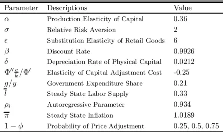
Table 1: Values of Preference and Technological Parameters

Parameter Descriptions Value

® Production Elasticity of Capital 0.36

¾ Relative Risk Aversion 2

² Substitution Elasticity of Retail Goods 6

¯ Discount Rate 0.9926

± Depreciation Rate of Physical Capital 0.0212

©^00e_k=©⁰ Elasticity of Capital Adjustment Cost -0.25

g=y Government Expenditure Share 0.21

l Steady State Labor Supply 0.33

½_i Autoregressive Parameter 0.934

¼ Steady State In°ation 1.0189

1¡Á Probability of Price Adjustment 0.25, 0.5, 0.75

3 Quantitative Properties

The equilibrium conditions are transformed in stationary variables and are log-linearized at the steady state.²⁵ After calibrating the model, we solved it recursively applying the method of King et al. (1987). Regarding the dynamic properties of the model, we ¯nd that the rational expectations equilibrium of the linear model is unique. Real determinacy is

21The value 0.25 for°is also choosen by Cooley aand Nam (1998) for their nominal business cycle model.

22Given the value of the elasticity², the ¯x costs of production can be calculated with:·= (²¡1)^¡1y:

23See, e.g., Jeanne (1998), and Gali and Monacelli (2000).

24These values for the fraction 1¡Áare also applied in Yun (1996).

25The log-linear model is presented in Appendix B.

10

Figure 1: Impulse Responses to a Positive Interest Rate Innovation (i; M=P; l; y) a robust feature of our model for several parameters variations over a range of reasonable values. This property is consistent with the results of Woodford (1994). He shows in a cash-in-advance economy that a combination of an interest rate peg and open market operations, which is comparable to our speci¯cation of monetary and ¯scal policy, leads to unique rational expectations equilibria. It should be noted that this kind of monetary and ¯scal policy is not proposed in order to avoid nominal indeterminacy, in the sense of Patinkin (1949) or Sargent and Wallace (1975), which commonly arises when the nominal interest rate is pegged.

3.1. Aggregate E®ects of Interest Rate Shocks

For an investigation of the particular transmission mechanism of the calibrated model, we computed the impulse responses of the model to policy shocks, i.e., innovations to the nominal interest rate rule (29). The impulse responses presented in this paper refer to percent deviations of the variables from their steady state values. The Figures 1-3 present impulse responses of the model for three di®erent degrees of price stickiness. Particularly, we vary the value of the probabilityÁfor the ¯rms of not receiving a price signal (Á= 0:25;

0:5;0:75), where a larger value ofÁindicates a higher degree of price stickiness.

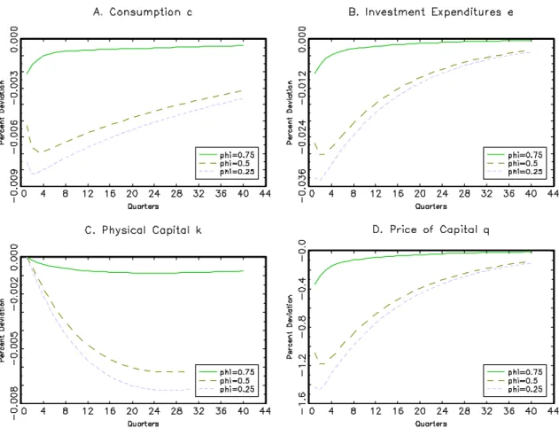
Figure 2: Impulse Responses to a Positive Interest Rate Innovation (c; e; k; q) Figure 1 and 2 present macroeconomic reactions to a nominal interest rate shock which are consistent with conventional expectations about monetary policy e®ects. Figure 1B displays that the monetary policy shock leads to a decline in liquidity, as the persistent rise in the nominal interest rate is associated with reduced holdings of real balances.

Induced by the increased cost of loans, the ¯rms' loan demand falls and employment declines (Figure 1C). Consequently, output falls immediately as can be seen from Figure 1D. Surprisingly, the decline in output is even stronger when prices are less sticky. This counterintuitive result is a direct consequence of the two main sources of non-neutrality which are jointly at work in this model. Lump-sum transfers, which are determined by the government budget constraint (31), rise as the negative amount of bonds is reduced while the nominal interest rate increases.²⁶ This expansionary impact is enhanced by higher degrees of price stickiness and leads to a smaller contraction in output which is caused by the working capital channel.

In equilibrium, the real contraction is accompanied by a reduced aggregate demand of the households. According to their cash constraint (3), the demand for both types of goods,

26The respective impulse response functions are presented in Appendix C.

12

i.e., the consumption and investment expenditures, fall symmetrically in response to the monetary contraction (Figure 2A and B). As a direct consequence of reduced investment expenditures, the price as well as the stock of physical capital decreases as shown in Figure 2C and D. Concerning the assets of the households, the portfolio adjustments can immediately be deduced from the aforementioned responses.²⁷ Consistent with the reduced real balance holdings and the associated open market exchanges, real bond holdings rise in response to the interest rate shock. At the same time the amount of deposits, which earn the same interest as bonds, is lowered as employment and wages fall in equilibrium as can be seen from the market clearing condition for intermediated funds (34).

Up to this point, it can be summarized that our model's responses to interest rate shocks are consistent with conventional wisdom and with VAR evidence. Regarding the aggregate production, the model predicts that output responds persistently and even in a hump-shaped manner in the case of moderate price stickiness. This pattern as well as the magnitude of the output response functions are comparable to the impulse response functions of typical VAR estimates.²⁸

3.2. Real Marginal Cost and In°ation

In the following subsection, we take a closer look at the responses of factor prices, real marginal cost and the in°ation rate to an interest rate shock. This strategy follows Barth and Ramey (2000) who study the impact of monetary policy shocks on ¯rms' optimal price setting in a partial equilibrium model. Their ¯rst order condition for the price setters corresponds to the forward looking pricing equation in our model which is derived from the conditions (20) and (21). This so-called 'New Keynesian Phillips Curve' states that the current in°ation depends on current real marginal cost and expected future in°ation:²⁹

b

¼_t =Âmc_ct+¯ E_t[b¼_t+1]; with >0; (35) wherebx(x=¼; mc) denotes the percent deviations from steady state valuex. For a given value of expected future in°ation, equation (35) predicts that in°ation should fall when real marginal cost decreases. According to the ¯rm's cost minimizing condition (17), real marginal cost depends positively on real factor prices and the nominal interest rate. The linearly transformed version of this condition is given by:

c

mc_t= (1¡®) i

1 +i^bi_t+ (1¡®)wb_t+®r_bt, with 0< ® <1: (36) Obviously, the behavior of in°ation depends on cost components (i; w; r) which may reveal di®erent responses after a monetary contraction. Given our monetary policy speci¯cation, a monetary tightening always tends to raise real marginal costs due to the rise in the nominal interest rate. Thus, for real marginal cost and, therefore, for the in°ation rate response it is decisive whether the factor prices, i.e., real wages w and the rental rate on capitalr, decline in response to a monetary contraction and to what extent.

27They are also displayed in Appendix C.

28See Bernanke and Mihov (1998), and Christiano et al. (1996, 1999).

29The parameter  depends on the probabilityÁ of receiving a price signal and the discount factor

¯:Â= (1¡Á) (1¡¯Á)Á^¡1(see Appendix A).

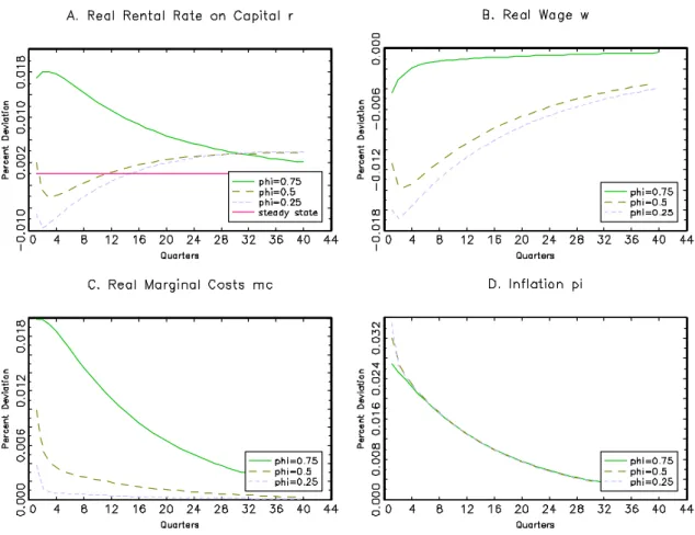
Given the standard properties of the production function (15), the decreased stock of physical capital tends to raise the rental rate on capital, while the latter is lowered by the decline in employment. Figure 3A reveals that these opposing e®ects result in a rising rental rate in the case of higher price stickiness (Á= 0:75), whereas the rental rate initially falls when prices are more °exible.³⁰ No matter which degree of price stickiness prevails, real wages always decline in response to a monetary contraction (Figure 3B).

When prices are not too sticky (Á < 0:75), both factor price reactions would predict a decrease of real marginal cost in the absence of interest payments on loans. In our model, the nominal interest rate does a®ect real marginal cost according to (36) and, as displayed in Figure 3C, causes a rise of the real marginal cost for all three degrees of price stickiness.

The increase in real marginal cost leads to declining real pro¯ts, as can be seen from the impulse response function of the ¯rms' pro¯ts in Appendix C. This feature of our model is consistent with empirical ¯ndings, which can not be replicated by a standard sticky price model with money growth shocks.³¹

The most remarkable property of the model's transmission mechanism is presented in Figure 3D. Here, it can be observed that the in°ation rate rises in response to a positive innovation to the nominal interest rate. It turns out that this behavior is persistent and robust. Moreover, after one year the responses of the in°ation rate are almost identical for all three degrees of price stickiness. Only in the ¯rst periods we ¯nd di®erences in the in°ation reactions which are small and opposed to the di®erences in the real marginal cost responses (Figure 3C). However, the response of in°ation in our model is consistent with the persistent rise in the price level commonly found in VARs when a sensitive price index is omitted.³²

So far, it can be proposed that it is the rise in the nominal interest rate as a cost component which is responsible for the unusual response of the in°ation rate to a monetary contraction. Barth and Ramey (2000) call this e®ect of monetary policy on the in°ation rate the 'Cost Channel of Monetary Transmission'. In general equilibrium, the rise in the in°ation rate is consistent with the household's arbitrage-free condition (10) which can be interpreted as a Fisher equation containing the variable priceq of physical capital. This

¯rst order condition for the household's asset holdings can be rewritten as:

E_t

·1 +i_t+1

¼_t+1

¸

=E_t

·(r_t+1+q_t+1³_t+1) q_t

¸

; (37)

with³_t= © µet

k_t

¶

¡©⁰et

k_t + (1¡±);

where ³ is positive and weighs the price of capital depending on the elasticity of the adjustment cost function ©.³³ The condition (37) claims that the expected value of the total real return on capital equals the expected real interest rate on bonds. Thus, when the total real return on capital is expected to fall in response to an increase in the nominal

30The divergence in the responses of the rental rate are due to the di®erent weights of the expansionary e®ect of rising lump-sum transfers. Since investments are assumed to be cash-goods, lump-sum transfers directly a®ect the price of capital as well as the rental rate on capital.

31See Christiano et al. (1997) for a critical discussion of sticky price models.

32See, e.g., Christiano et al. (1996).

33Obviously,³is equal to 1¡± in the steady state.

14

Figure 3: Impulse Responses to a Positive Interest Rate Innovation (r; w; mc; ¼) interest rate, the expected value of the in°ation rate must rise in order to ensure the equality.³⁴ This implies that, holding the other variables constant, higher expected values of the rental rate r should be accompanied by lower expected values of in°ation. This pattern can be observed in Figure 3A and D.

4 Conclusion

The majority of monetary business cycle models treats a broad monetary aggregate as an exogenous policy measure of the central bank, whereas in the empirical literature the federal funds rate is mostly applied as the policy measure. This paper tries to overcome this disparity and presents a monetary business cycle model which allows to examine the e®ects of innovations to a non-contingent nominal interest rate rule while ensuring real determinacy. In addition to a working capital assumption we consider staggered price setting which enables real marginal costs to vary. It is shown that the model is able to replicate typical responses to interest rate shocks of monetary VARs. Consistent with Barth and Ramey's (2000) 'Costs Channel of Monetary Transmission', we particularly ¯nd

34This argument is con¯rmed by the impulse response of the real return on bonds given in Appendix C.

that real marginal costs and in°ation rise in response to positive interest rate innovation.

As the model's transmission mechanism provides a rationale for the so-called price puzzle in monetary VARs, we suggest that the latter should not be treated as an empirical anomaly. Obviously, this result is incompatible with conventional monetary theory and should not be taken as an advice to rethink monetary theory. Though, it casts doubt on the appropriateness of the measures for an unanticipated change in monetary policy, which are applied in this model and in many VARs.

16

Appendix

Appendix A: Derivation of the New Keynesian Phillips Curve

We start by linearizing equation (21), which determines the evolution of the price index P. For this, it is transformed in stationary variables:

1 =

·

Á^³¼¼^¡_t^1´1¡²+ (1¡Á)P^e_qt^1¡²

¸ ¹

1¡²

;withP^e_qt =P^e_it

P_t and ¼_t = P_t

P_t¡1; (A1) where bxdenotes the percent deviation ofxfrom its steady state value x. Linearization of (A1) at the steady state leads to:

Á

1¡Á^b¼_t =P^be_qt. (A2)

Further, we need the ¯rst order condition for the ¯rm's optimal price P^e_it (20). For the linearization at the steady state, it is also transformed in stationary variables:

Pe_qt²¡1

² X1 s=0

(¯Á)^sE_t^h#_t;t+sy_t+s¼^²_t;t+s¼^(1¡²)si= X1 s=0

(¯Á)^sE_t^h#_t;t+sy_t+s¼^²+1_t;t+smc_t+s¼^¡²si; (A3) where ¼_t;t+s denotes a cumulative in°ation rate: ¼_t;t+s = ^P_P^t+s_t =^Qs

k=1

¼_t+k: Linearizing equation (A3) at the perfect foresight steady state we obtain:

X1 s=0

(¯ Á)^sP^e_q²¡1

² y¼^(1¡²)s¼^s(²¡1)E_t

·#b_t;t+s+y_bt+s+²¼_bt;t+s+P^be_qt

¸

(A4)

= X1 s=0

(¯ Á)^smcy¼^¡²s¼^s²E_t^h#b_t;t+s+y_bt+s+ (²+ 1)¼_bt;t+s+mc_ct+sⁱ:

Using that P^e_q^²¡_²¹ = mc holds in the steady state and substituting P^e_q out with (A2), equation (A4) can be simpli¯ed to:

Á

(1¡Á)¼^b_t = (1¡¯Á) X1 s=0

(¯Á)^sE_t[_b¼_t;t+s+mc_ct+s]: (A5)

Taking the period t+ 1 expression for equation (A5) times ¯Á and substracting it from (A5), gives:

Á

(1¡Á)(b¼_t¡¯ÁE_t[b¼_t+1]) = (1¡¯Á) Ã

c mc_t¡¯Á

X1 s=0

(¯Á)^sE_t[¡¼b_t+1]

!

: (A6)

Equation (A6) can then be rewritten, leading to the 'New Keynesian Phillips Curve' in (35):

b

¼_t =Âmc_ct+¯E_t[¼b_t+1]; withÂ= (1¡Á) (1¡¯Á)Á^¡1: (A7)

Appendix B: The Log-linear Model State variables: k_t,m_t´ _P^M_t¡1^t ; b_t= _p^B_t¡1^t Costates: ¸_t,q_t; pi

Control variables: c; l; e; w; r; z; ¿; mc Exogenous states: i

Dynamic Equations:

k^_t+1¡(1¡Á⁰e

k)^k_t=Á⁰(:)e

k^e_t (A8)

¯Á⁰⁰ µe

k

¶2

^kt+1+ ^¸t+1+¯ µ

1¡Á⁰e k

¶

^

qt+1¡¸^t¡q^t=¯Á⁰⁰ µe

k

¶2

^

et+1¡¯ qr^rt+1

¡¸^t+1+ ^¸t+ ^¼t+1= i 1 +i^it+1

^b_t+1= ¿

¿+g¿^b_t¡ 1 1 +i^i_t+1

¡ Á

(1¡Á) (1¡¯Á)¯¼_bt+1+ Á

(1¡Á) (1¡¯Á)¼^b_t=mcc_t mm_bt+1+b^b_t+1¡m

¼m^b_t¡ b

¼^b_t+

µm+b

¼

¶

^

¼_t= 0 Contemporaneous Equations:

[(1¡¾)°¡1] ^c_t¡(1¡¾)(1¡°) l

1¡l^bl_t=¸^b_t+ i

1 +i^i_t (A9)

(1¡¾)°^c_t¡[(1¡¾)(1¡°)¡1] l

1¡l^bl_t¡wb_t=¸^b_t+ i 1 +i^i_t ee_bt+c_bc_t¡wl^bl_t¡wlw_bt+zz_bt=m

¼m^b_t¡m

¼^b¼_t

®^l_t+ ^w_t¡mcc_t=®k^_t¡ i 1 +i^i_t

¡(1¡®)^l_t+ ^r_t¡mcc_t=¡(1¡®)^k_t Á⁰⁰

Á⁰ e

ke^_t=Á⁰⁰ Á⁰

e

k^k_t¡q^_t+ i 1 +i^i_t c

y^c_t¡(1¡®)^l_t+ e

ye^b_t=®^bk_t wl^l_t+wlw^_t¡z^z_t+¿¿_bt= 0

18

Appendix C: Additional Impulse Response Functions

Impulse Responses to a Positive Interest Rate Innovation (B=P; ¿; d; z;(1 +i)¼^¡1;-^f=P).

Note that, the impulse responses of government transfers and real bonds indicate increases as the steady state values are negative. The responses of the pro¯ts are given in absolute values.

References

Barth, Mike, and Valerie, Ramey, 2000, The Cost Channel of Monetary Transmis- sion, NBER Working Paper, no. 7675.

Benhabib, J., Schmidt-Grohe, S. and M. Uribe, 1998, Monetary Policy and Mul- tiple Equilibria, Manuscript, New York University.

, , and , 1999, The Perils of Taylor Rules, Manuscript, New York University.

Bernanke, B.S., M. Gertler, and S. Gilchrist, 1998, The Financial Accelerator in a Quantitative Business Cycle Framework, NBER Working Paper, no. 6455.

Bernanke, B.S., and I. Mihov, 1998, Measuring Monetary Policy, Quarterly Journal of Economics, 869-901.

Bergin, P., and R.C. Feenstra, 1998, Staggered Price Setting and Endogenous Per- sistence, NBER Working Paper, no. 6429.

Calvo, G., 1983, Staggered Prices in a Utility-Maximizing Framework, Journal of Mon- etary Economics, vol. 12, 383-398.

Carlstrom, C.T., and T.S. Fuerst, 1995, Interest Rate Rules vs. Money Growth Rules:

A Welfare Comparison in a Cash-in-advance Economy, Journal of Monetary Eco- nomics, vol. 36, 247-267.

, and , 2000, Money Growth Rules and Price Level Determinancy, Working Pa- per, Federal Reserve Bank of Cleveland.

Casares, M., and B. McCallum, 2000, An Optimizing IS-LM Framework with En- dogenous Investment, NBER Working Paper, no. 7908.

Chari, V.V., P.J. Kehoe and E.R. McGrattan, 1996, Sticky Price Models of the Business Cycle: Can the Contract Multiplier Solve the Persistence Problem?, Re- search Department Sta® Report 217, Federal Reserve Bank of Minneapolis.

Christiano, J.L., and M. Eichenbaum, 1992, Liquidity E®ects and the Monetary Trans- mission Mechanism, American Economic Review, vol. 82, 346-53.

Christiano, J.L., M. Eichenbaum, and C.L. Evans, 1996, The E®ects of Monetary Policy Shocks: Evidence from the Flow of Funds, Review of Economics and Statistics, vol. 78, 16-35.

, , and , 1997a, Sticky price and Limited Participation Models of Money: A Comparison, European Economic Review, vol. 41, 1201-49.

, , and , 1999, Monetary Policy Shocks: What Have We Learned and to What End?, in: M. Woodford and J.B. Taylor (eds.), Handbook of Macroeconomics, Am- sterdam: North-Holland.

20