Animal Spirits, Technology Shocks and the Business Cycle

(1)

SHOCKS AND THE BUSINESS CYCLE

Mark WEDER

July 1, 1997

Abstract

In this paper a two-sector growth model allowing indeterminacy to occur at relatively mild degrees of increasing returns is developed. It is shown that these economies of scale need only be present in one sector of the economy (investment). This feature of the model, therefore, builds on evidence that was recently reported by Basu and Fernald (1996). The model is also able to solve some puzzles of business cycle research which standard Real Business Cycle models have not been able to. The introduction of animal spirits generates a low negative contemporaneous correlation of hours and productivity as well as a procyclical investment share. The model can account for the observed variability of hours worked.

Keywords: Sunspots, technology shocks, economic uctuations, Dunlop-Tarshis- puzzle.

Journal of Economic Literature Classication: E00, E32.

Humboldt University Berlin, Department of Economics, Spandauer Str. 1, 10178 Berlin, Germany, weder@wiwi.hu-berlin.de.

I am indebted to Michael Burda for his guidance. I would like to thank Jess Benhabib, Dalia Marin, Ellen McGrattan, Harald Uhlig, Thomas Sargent, Rolf Tschernig and par- ticipants of the 1996 Summer School of the European Economic Association for valuable comments. All remaining errors are mine.

1

(2)

Animal Spirits, Technology Shocks and the Business Cycle 2

1 Introduction

The last few years have witnessed a revival of business cycle models in which beliefs of agents (or animal spirits) have played a leading role in explaining economic uctuations.¹ Most of these models involve strong economy-wide increasing returns to scale in order for sunspot equilibria to exist. In a recent paper, however, Basu and Fernald (1996) present evidence that returns to scale are far from evenly distributed across the U.S. economy. In particular,they report that scale economies are present mainly in the domain of durable goods production. In the nondurable goods sector of the U.S.

economy evidence of increasing returns to scale cannot be found.

The innovation of this paper is to demonstrate that Basu and Fernalds's (1996) ndings can be used within a two-sectoral optimal growth model to generate non-uniqueness of rational expectations equilibria. It is assumed that each of the two sectors produces a list of intermediate consumption goods or investment goods respectively. The number of these goods is xed and each intermediate good is produced by one industry each. I consider Cournot competition in each industry. Endogenous entry and exit of rms in each product's industry results in a variable mark up. Indeterminacy arises at returns to scale of around 1.15 in the investment sector alone. This indeterminacy can then be exploited so that animal spirits can be introduced as a driving variable in order to generate cyclical behavior of the model as in Farmer (1993).

Although the debate on business cycles was revived as a result of the new literature on self-fullling expectations, it is indisputable that recent developments have failed to produce a widely accepted paradigm as of today.

The principal problem of the mentioned work is the dependency on degrees of scale economies and market power that are not suggested by (most) empirical studies. The exception is Benhabib and Farmer (1996) who seem to have found an escape out of this dilemma. They are able to show that by working with a two-sector optimal growth model the extent of increasing returns that is needed to obtain indeterminacy can be reduced signicantly.² The principal dierence between their work and mine is that these authors do not

1See for example Farmer (1993), Farmer and Guo (1994), and Schmitt-Grohe (1995).

2The abnormal behavior of two-sector growth models was already examined in the sixties (for example Shell, 1967).

(3)

Animal Spirits, Technology Shocks and the Business Cycle 3 consider any asymmetry of scale economies of the sort reported by Basu and Fernald (1996). A further distinction is that they do not use oligopoly as I do.Technology shocks will not be dismissed as a source of economic uctuations in this work altogether. I will entertain the idea of a coexistence (and coimportance) of both shocks in the economy as in Farmer and Guo (1995) and others.³ They have found that demand and supply shocks account for about the same magnitude in explaining business cycles in the U.S. post-war period. Another reason for considering two simultaneous shocks was given by McGrattan (1994), Baxter and King (1991) and others. According to McGrattan, the major problems of the standard Real Business Cycle model are the predictions of variability of hours and the impossibility to account for the Dunlop-Tarshis puzzle.⁴ These decits can be overcome once additio- nal disturbances (to technology shocks) are introduced. McGrattan (1994) assumes stochastic taxation as well as shocks to government expenditures.

Baxter and King (1991) obtain a similar result when preference shocks are introduced into the Real Business Cycle model. Both of these works are able to generate a low correlation of hours and productivity.⁵ The intention of this work is to demonstrate that these and other complications of Real Business Cycle models can also be solved within a general equilibrium model in which both animal spirits and technology shocks are the forcing variables.

The paper proceeds as follows: Section 2 presents the model. The economy's steady state and its dynamics around it will be derived in section 3. In section 4 the model is calibrated. This is followed by two exercises the rst will establish parameter constellations at which indeterminacy is possible and the second will compute model statistics to assess the model's business cycle properties (sections 5 and 6). Section 7 concludes the paper.

3See for example Gerlach and Smets (1995).

4The Dunlop-Tarshis puzzle implies that real wages and labor input move acyclical to each other.

5Christiano and Eichenbaum (1992) consider stochastic government expenditures plus technology shocks.

(4)

2 The model

The economic model developed is a two-sector extension of a baseline Real Business Cycle model as in, for example, King, Plosser and Rebelo (1988).⁶ It is assumed that the markets for investment goods and consumption goods are characterized by oligopoly.⁷

2.1 The household

I will assume that the economy consists of a representative household. The household supplies labor and capital services to the rms on competitive markets. I assume that the representative agent has expected lifetime utility

E^X¹

t=0 t

U(^C^t^l^t)^jÎ^t] (1) whereÛ(^:) is instantaneous utility,^C^tis a consumption index,^l^tleisure time, the discount factor and Î^t the set of information available at ^t. Consump- tion of the households is dened by a CES-aggregator over all dierentiated goods available (normalized to unity):

C

t= (

Z

1

0 C

ct

dc)¹⁼ ^: (2)

The number of consumption goods is constant. Consumption is a function of the consumption level of an assembled variety of the dierentiated goods indexed by ^c. Each of these goods enters the aggregator symmetrically. For

< 1, the goods are imperfect substitutes. Analogously to the denition of the consumption bundle, an aggregator for the investment good, ^I^t, is dened. Again it is a CES-function of the purchases of the dierentiated products:

I

t= (

Z

1

0 I

it

di)¹⁼^: (3)

6See also Christiano and Fisher (1995).

7Another work which includes oligopoly in the Real Business Cycle framework is Gali (1995).

(5)

Animal Spirits, Technology Shocks and the Business Cycle 5 The number of investment goods is constant. The period-by-period budget constraint of the household is given by

Z

1

0 p

cct C

ct dc+

Z

1

0 p

iit I

it

di=^w^t^L^t+^q^t^K^t+ ^t^: (4) Here ^p^cct (^p^iit) is the price of the consumption (investment) good ^c (ⁱ).

Both prices are taken as given for the households. ^w^t is the nominal wage.

Furthermore, the household receives prot income from all existing rms ^t. Households own the stock of capital ^K^t and rent it out to the rms at the rental price ^q^t. All factor prices and prot income are taken as given for the households. Households are endowed with one unit of time per period which they can either use for leisure or work ^L^t:

1 =^L^t+^l^t^: (5)

The following specic functional form for periodic utility is assumed:

U(^C^t^L^t) = log^C^t+1 +^B^l¹⁺^t with 0^: (6)

B is a constant. The consumer's capital holdings evolve as

K

t+1 = (1^;)^K^t+^I^t (7) where is the rate of depreciation. The household maximizes (1) subject to (4), (5) and (7). As is well known for this class of models, maximization can be conducted as a two step procedure. The current-periodic household expenditure functional of consumption goods subject to ^C^t is given by

E(^p^cct^C^t) =^C^t(^Z ¹

0 p

1;

cct

dc)^1; (8)

where ^p^cct is a function of the consumption goods' prices. By applying Shephard's Lemma in the rst step, the conditional demand can be derived as

C

ct= (^p^cct

p

ct

) ^;1¹ ^C^t (9)

(6)

Animal Spirits, Technology Shocks and the Business Cycle 6 which has a constant price elasticity. Here

p

ct (

Z

1

0 p

;1

cct

dc) ^;1 (10)

is the exact price index for the consumption goods. The conditional demand becomes

I

it= (^p^iit

p

it

)^;1¹ ^I^t (11)

and

p

it

(^Z ¹

0 p

;1

iit

di)^;1 ^: (12)

Given the conditional demands, I am able to derive the intertemporal optimality condition for the household. In symmetric equilibrium, the only case to be considered in this paper, the household buys the same amount of every product: ^C^ct = ^C^t (and Îît = Î^t). The prices of all goods equal. Finally, I use the price of the consumption goods in equilibrium as the numeraire and, without loss of generality, normalize it to unity. The budget constraint transforms into

C

t+^p^t^I^t =^w^t^L^t+^q^t^K^t+ ^t^: (13)

p

t can be interpreted as the relative price of investment goods in symmetric equilibrium.

The second step of the household's optimization program consists of com- puting the optimal path of spending and working. Each household chooses a sequence ^fC^t^L^t^K^t+1^g¹^t=0 subject to ^K⁰ and to the distribution of technology innovations (see below). The rst order conditions can be written as

8

C

;1

t

;

t = 0 (14)

B(1^;^L^t)^;^t^w^t= 0 (15)

8Here ^t is the current value Lagrange multiplier associated with the household's re- source constraint.

(7)

E^t+1(^q^t+1+ (1^;)^p^t+1)^j^I^t]^;^t^p^t = 0 (16) plus the household's period-by-period budget constraint

w

t L

t+^q^t^K^t+ ^t^;^C^t^;^p^t^I^t= 0 (17) and the transversality condition

lim

s!1

E ^t+s;1^t+s;1^K^t+s ^j^I^t] = 0^: (18) (14) and (15) describe the household's consumption-leisure trade o and (16) is the standard intertemporal optimality condition.

2.2 The rms

One signicant modication of conventional Real Business Cycle modelling is considered: I assume that consumption and investment goods are produced in two distinct sectors. Households can move their labor and capital services freely and without costs between the two sectors.⁹ It is also assumed that product markets are oligopolistic. Factor prices are given for the individual rm and household.

2.3 The consumption goods sector

The part of the economy that produces consumption goods consists of subsectors, each producing a dierentiated product. The measure of subsectors is normalized to one.¹⁰ There are ^N^ct rms supplying their single good ^j every period ^t. Each rm ^j supplies its product in sector (market) ^c under the assumption of Cournot competition. ^N^ct must not necessarily be constant. Costless endogenous entry and exit of rms will be allowed.

Firm's^joutput^Y^cjtis related to capital input^K^cjt and labor input^L^cjt according to the production function

Y

cjt =^C^cjt =^Z^t(^K^cjt ^L^1;^cjt) ^; (19)

9A possible and realistic extension of the model would be the introduction of limited mobility of labor and capital.

10Basically both sectors of the economy are the same in structure. Therefore, only the sector that is discussed rst is described in detail.

(8)

Animal Spirits, Technology Shocks and the Business Cycle 8 where is overhead costs. ^Z^t is the state of technology which evolves as

log^Z^t+1 = log^Z^t+^z^t+1 0^< ^<1^:

Units have been chosen to make the conditional mean ^E^Z^t] = 1. The sequence^fz^t^gis a normally distributed white noise process with zero mean and constant variance^z². Given the assumption on the form of competition, the rm's program can be written in the specic Cournot form

max ^cjt = (^C^c;jt+^C^cjt

C

t

) ^;1^p^ct^C^cjt^;^w^t^L^cjt^;^q^t^K^cjt (20) subject to its production function (19). ^p^cjt is the price of the rm's^j good (in market ^c) and ^C^c;jt is the supply of all other rms in sector ^c which is taken as given for every rm^j. The cost function of rm^j is given by

C(^w^t^q^t^C^cjt) =^Aq^t^w^1;^t (^C^cjt+

Z

t

)¹ (21)

where the constant ^A is dened as ^A (^1; )^1; + (^1; )^;. Each rm ^j maximizes its prots (20) given the quantity supplied by others. Optimality requires that

(^;1)^p^cjt(^C^c;jt+^C^cjt)^;1^C^cjt+^p^cjt (22)

= ^A^Zt^q^t^w^1;^t (^C^cjt^Zt⁺)¹^;1

holds. (22) equalizes marginal revenues and marginal costs. Marginal costs are decreasing (increasing) for ^> 1 ( ^< 1). At every period in time the number of active rms is implicitly determined by the zero prot condition

p

cjt C

cjt =^Aq^t^w^1;^t (^C^cjt+

Z

t

)¹^: (23)

Inserting the optimal pricing rule into the zero prot condition yields

p

cjt C

cjt =((^;1)(^C^c;jt +^C^cjt)^;1^p^cjt^C^cjt+^p^cjt)(^C^cjt+)^: (24) In symmetric equilibrium^N^ct^C^cjt =^C^ct =^C^t,^N^ct=^N^tand^p^cjt =^p^ct = 1 hold, where the last equality follows from the normalization that was already

(9)

Animal Spirits, Technology Shocks and the Business Cycle 9 made in section 2. Equation (24) has the aggregate correspondence in symmetric equilibrium of¹¹

C

t =(^;1

N

t

+ 1)^Z^t^K^ct^L^(1;)^ct ^N^t^1;^: (25) The term 1 + ^Nt^;1 is the inverse of the markup in the consumption goods sector. Note that the markup is decreasing inwhich implies that a low spe- cialization of the input goods translates into a low degree of market power.

The markup is also decreasing in the number of rms. That is, the model predicts a countercyclical pattern of the markup. This is supported by empirical evidence summarized by Rotemberg and Woodford (1991).¹²

Combining the optimal markup rule (22) with the conditional demand for labor, it is possible to derive the (equilibrium) wage rate as

w

t = (1^;)(1 + ^;1

N

ct

)^Z^t(^K^cjt ^L^1;^cjt)^L^;1^cjt^: (26) Accordingly, the rental rate of capital is given by the term

q

t=(1 + ^;1

N

ct

)^Z^t(^K^cjt ^L^1;^cjt)^K^cjt^;1 ^: (27) Note that this simple aggregation of the conditional demands does not yet yield the actual rental prices. These demands must be combined with the equilibrium value for ^N^ct, as given by the zero prot condition.

2.4 The investment goods sector

There are ^M^it rms supplying their respective investment good ^j in sector (market) ⁱ every period ^t.¹³ The market structure and the production

11Equation (25) can be rewritten as

C

t= (^;1 +^N^t) 1^;( ^N^;1t + 1)

which states, for example, that for a given number of rms^N^t, a rise of overhead costs must be met by a rise in sales of consumption goods ^C^t (otherwise the number of rms must decrease). Also, a fall in and a fall in^N^tincreases the production of consumption goods.

12See also Burda (1985).

13Again the letter^j denotes the individual rm.

(10)

Animal Spirits, Technology Shocks and the Business Cycle 10 technology in the investment goods sector are essentially the same as in the consumption goods sector. Each rm^j supplies its product in sector ^j under the assumption of Cournot competition. It operates under the technology

Y

ijt =Îîjt=^Z^t(^Kîjt ^L^1;îjt)^;;^: (28) HereÎîjtis the amount of output to be sold by the^jthrm in sectorⁱ. ^Kîjt and ^Lîjt are capital and labor input of rm^j at^t. ; is overhead costs when operating the rm. Each rm^j solves

max îjt = (Îî;jt+Îîjt

I

t

)^;1^pîtÎîjt^;^C(^w^t^q^tÎîjt) (29) where Îî;jt is the supply of all other rms in sector ⁱ. The sequence of deriving a rm's optimal program in the investment sector is the same as in the consumption sector. Again the number of equilibriumrms is determined by free entry and exit. In symmetric equilibrium, the zero prot condition is given by

I

t=(^;1

M

t

+ 1)^Z^t^K^it^L^(1;)^it ^M^t^1;^: (30) The optimal inverse factor demands are implicitly determined (in symmetric equilibrium) by

w

t= (1^;)^p^t(1 + ^;1

M

t

)^Z^t(^K^it^L^1;^jt )^M^t^1;^L^;1^it (31) and

q

t=^p^t(1 + ^;1

M

t

)^Z^t(^Kît^L^1;ît )^M^t^1;^Kît^;1^: (32)

2.5 Factor markets in symmetric equilibrium

By combining (14), (15), (25) and (26), labor input in the consumption goods sector is given as

(1^;)^L^;1^ct =^B(1^;^L^t)^: (33)

(11)

Animal Spirits, Technology Shocks and the Business Cycle 11 As long as ⁶= 0, ^L^ctand ^L^t move in opposite directions, labor input in the consumption sector is countercyclical. This is an unrealistic feature of any two-sector optimal growth model with endogenous labor supply.

The continua of rms in the two sectors rent factor services from the same market. Combining the factor market clearing conditions (26), (27), (31) and (32) yields an equalization of factor intensities in the form

K

ct

L

ct

= ^K^it

L

it

= ^K^t

L

t

: (34)

Finally I dene overall sales ^Y^t as the measure of output in the economy.¹⁴ Sales are given by

Y

t =^C^t+^p^t^I^t^: (35)

3 The equilibrium dynamics

This section describes the steady state and the dynamics of the model economy.

3.1 The steady state of the economy

The steady state is given by the following list of equations (36 to 40). Omit- ting the time index refers to steady state variables.

;1

p=^q+ (1^;)^p (36)

=^I^=K (37)

N

C

= ^N ^;(^;1 +^N)

(^;1 +^N) (38)

;^M

I

= ^M ^;(^;1 +^M)

(^;1 +^M) (39)

14In this model I measure aggregate economic activity by sales and not by overall production which would include the overhead. However, it can be shown that the general results are not aected by the particular choice of an output measure.

(12)

Animal Spirits, Technology Shocks and the Business Cycle 12 Equations (36) and (37) are generally found in Real Business Cycle models.

(38) and (39) can be interpreted as follows: both equations are the steady state versions of the zero-prot condition for each of the two sectors in the economy. The left hand side is the ratio of overhead to output in each sector.

(38) can be interpreted as follows: assume a rise in, that is, a lower market power for each rm in the consumption sector market, implying that the left hand side of (38) must decrease. For a given overhead and ^C, the steady state number of rms falls. The same result occurs for an increase in and

(). For a given overhead and ^C, the steady state number of rms falls.

Similar results occur for an increase in or ().

3.2 The solution mechanism

The following section describes the dynamics of the economy near its steady state. Since the Second Welfare Theorem does not apply because of the existing market power, the dynamics cannot be derived by means of the social planner problem. I therefore use the solution method described by King, Plosser and Rebelo (1988), which involves approximating the necessary and sucient rst order conditions into a rst order linear system.¹⁵

Dene the vector ^^t according to¹⁶

^^t= ^^C^t^Y^^tÎ^^t^w^^t^q^^t^L^^t^L^^ct^L^ît^K^^ct^K^ît^N^^t^M^^t]⁰^: (40) The vector of controls is related to the relative price, to the capital stock and to the technology (the vector of states) as

J

1^^t =^J²

2

4

^

p

^t K

^t Z

t 3

5 (41)

where^J¹and^J² are 1212 and 123 matrices respectively. The loglinearized versions of the Euler equation, the budget constraint as well as the technology process relate variations in ^^p, ^^K and ^^Z to changes in ^^t:

J

3(^L)

2

4

E^^p^t+1^j^I^t]

^

K

t+1

E ^^Z^t+1 ^j^I^t]

3

5=^J⁴(^L)^^t+1 (42)

15See also Woodford (1986) and Uhlig (1995) for justications of this method.

16Û^^t denotes the percentage deviation of the variableÛ^tfrom its steady state valueÛ at^t.

(13)

Animal Spirits, Technology Shocks and the Business Cycle 13 where the^J^j(^L)s are matrix polynomials in the lag operator^Lat most power of one. The last two equations can be combined to yield

2

4

E^^p^t+1^j^I^t]

^

K

^t+1 Z

t+1 3

5=^J

2

4

^

p

^t K

^t Z

t 3

5+

2

4

00

z

t+1 3

5 (43)

where ^J is 33. A three-dynamical system describes the economy's dynamics. The eigenvalues of ^J must be evaluated at the steady state. The system contains: one predetermined variable, the stock of capital, ^^K^t, one endogenous (nonpredetermined) variable, ^^p^t, and one exogenous (nonpredetermined) variable, ^^Z^t. Thus, if all eigenvalues of ^J are inside the unit circle, the rational expectations equilibrium is non-unique. This will be analyzed in the following section. The calibration method will be applied to check if indeterminacy has realistic relevance.

4 Calibration

Parameter value determination will follow in the Real Business Cycle tra- dition. Steady state values of the model will be matched with estimates of average growth rates and ^{gr eat} ^{r atios}. First a baseline model structure will be dened. Without setting xed values for all variables, the regions of realistic calibrations will be shown.

To calibrate the model as close as possible to established Real Business Cycle theory, I will set parameters as proposed in existing studies. Quarterly

is equal to 0.025 and (the capital share) is set at 0.36, which is standard in Real Business Cycle models (see for example Hansen, 1985).

Basu and Fernald (1995) report estimates for increasing returns from 1.00 to 1.26. However, their preferred point estimate is 1.03. In their work, the regression was restricted by assuming that returns to scale are the same over the economy. Basu and Fernald (1996) show that economies of scale are largely heterogenous across the economy, however. For durable goods manu- facturing, they report signicant increasing returns with a point estimate of 1.36 (their Table 3).¹⁷ For the production of nondurables, on the other hand,

17Depending on various estimation methods, the point estimate ranges from 1.07 (still signicantly dierent from one) to 1.46.

(14)

Animal Spirits, Technology Shocks and the Business Cycle 14 (insignicant) diminishing returns are reported. Based on these results, it will be assumed that the consumption sector in the present model displays close to constant returns. This is a key assumption in this paper. These values restrict the region of the parameter space in which a realistic calibration can be undertaken.

The markups over marginal cost are given by 1

MC

= ^N

;1 +^N for the consumption goods sector and by

P

MC

= ^M

;1 +^M

for the investment goods sector. The last two equations each possess one degree of freedom. For example, if I x both the markup and in the consumption goods sector, the number of steady state rms ^N is uniquely determined. The same holds for the investment goods sector.

Information does not exist in the empirical literature concerning the magnitude of the elasticity of substitution of investment and consumption goods in the aggregate. In models of monopolistic competition, the elasticity of substitution and the markup are interdependent since they are exactly inverse to each other. Consistent with the assumption of Cournot competition, the markup also depends on the number of incumbent rms. Basu and Fer- nald report markup margins from 1.00 to 1.26. Morrison (1990) reports the markup to be around 1.14. However, all of theses authors assume that the markup is homogenous over the economy. In light of the mentioned evidence in Basu and Fernald (1996), I will assume that the markup in the investment goods sector signicantly exceeds the one in the consumption goods sector.

Choosing a value for the steady state markup then determines the number of rms in the respective sector. I further assume that the inverse of () always equals the markup as a normalization.

I assign a value of^L= 1⁼3, implying that the representative agent spends on average one third of her time endowment working (see also Hansen, 1985).

Note that in the case of = 0, the model's labor market corresponds to the Hansen (1985) and Rogerson (1987) indivisible labor market formulation.

Labor supply becomes innitely elastic. At =^;1⁼2, the model possesses

(15)

Animal Spirits, Technology Shocks and the Business Cycle 15 a labor supply elasticity of 4, which is the same as in the King, Plosser and Rebelo (1988) baseline Real Business Cycle model.

Next I will calibrate the ratio of consumption to output in the model economy. Kydland and Prescott (1990) report that total consumption expenditures amount to 80 percent of output net of government expenditures.

If only expenditures on nondurables and services are considered, the ratio falls to 68 percent. I will x the ratio of consumption to overall expenditures at 75 percent. This is done by adjusting the preference parameter^B.

The rate of return in the model is given by

r

t+1= ^q^t+1+ (1^;)^p^t+1

p

t

;1 which implies in steady state

r= ^q

p

;= 1 ^;1

where the last equality follows from (36). I set discount rate = 0^:99.

This assumption is standard in Real Business Cycle models. Using the last equation, the choice implies a rate of interest of four percent. ^Kⁱ can be computed from

r= ^q

p

; =(^;1

M

+ 1)^Kⁱ^;1^L^(1;)ⁱ ^M^1;^;^:

K

c is given by ^Kⁱ^L^c^=Lⁱ.

5 Results

In the rst part of this section, I will evaluate the regions of parameter constellations in which indeterminacy can arise. Second moments are derived in the latter part of the section.

5.1 Eigenvalues

The occurrence of indeterminacy will be analyzed rst. Indeterminacy is present in the model as long as both roots of the matrix^J are inside the unit

(16)

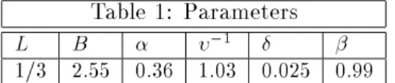
Animal Spirits, Technology Shocks and the Business Cycle 16 circle. However, since the analytical solution of the matrix ^J is muddled, a numerical procedure is considered here. Table 1 considers the parameters which are not changed in the analysis unless otherwise noted.

Table 1: Parameters

L B

;1

1/3 2.55 0.36 1^:03 0.025 0^:99

Considering the assumptions made, Table 1 implies that the markup in the consumption sector is equal to 1.03. This value is also the measure of increasing returns in this sector (see also the Appendix).¹⁸ A certain degree of scale economies is assumed to justify market power in the consumption goods sector. The choice for ^B implies a consumption share of around 75 percent (the exact value depending on the remaining calibration).

The parameter space in which indeterminacy arises will be reported. Ta- ble 2 displays regions for indeterminacy for alternative values of scale econo- miesin the investmentgoods sector. The labor marketfollows Hansen (1985), that is = 0. Marginal cost are constant in both sectors: == 1^:00.

Table 2: Roots of Model

;1 Root 1 Root 2 stability

1.10 1.108 0.926 saddlepath stable

1.225 0.810+0.225 i 0.810-0.225 i stable 1.25 0.945+0.148 i 0.945-0.148 i stable 1.30 0.977+0.098 i 0.977-0.098 i stable 1.35 0.985+0.078 i 0.985-0.078 i stable 1.40 0.989+0.067 i 0.989-0.067 i stable 1.45 0.992+0.059 i 0.992-0.059 i stable

Table 2 shows that the present model does not require unrealistic scale

18It can be shown that the results reported in this paper are not dependent on the numerical choice of. The basic features of the model carry over for dierent calibrations of. In particular,^!1 does not pose any problems for the results that are reported in this paper.

(17)

Animal Spirits, Technology Shocks and the Business Cycle 17 economies in order to produce indeterminacy.¹⁹ The model is indeterminate at increasing returns to scale in the investment goods sector of ^;1 = 1^:22.

Existing one sector animal spirits models which were summarized in Schmitt- Grohe (1995) require increasing returns in excess of 1.75 for variable markups and 2.31 for constant markups if the models were calibrated in the same way as in the present model.²⁰ This result therefore indicates an improvement to previous work.

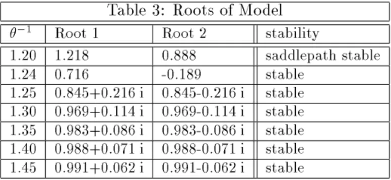
Table 3 repeats the analysis for nonconstant marginal costs. In particular, it is assumed that marginal costs are increasing: == 0^:95.

1.24 0.716 -0.189 stable

1.25 0.845+0.216 i 0.845-0.216 i stable 1.30 0.969+0.114 i 0.969-0.114 i stable 1.35 0.983+0.086 i 0.983-0.086 i stable 1.40 0.988+0.071 i 0.988-0.071 i stable 1.45 0.991+0.062 i 0.991-0.062 i stable

This Table shows that indeterminacy is possible with upward sloping marginal costs schedules. The minimum required returns to scale is still not outside of what is considered realistic.

Table 4 considers diminishing marginal costs in the investment sector,

= 1^:10 (and = 1^:00).

19The matrix^J contains a third root which equals the parameter . Since technology is assumed to be stationary, the third root is always inside the unit circle and is not reported in the Tables.

20In particular concerning the labor supply elasticity and the assumption on the value of.

(18)

1.14 0.700 0.028 stable

1.15 0.811+0.225 i 0.811-0.225 i stable 1.20 0.963+0.125 i 0.963-0.125 i stable 1.25 0.980+0.091 i 0.980-0.091 i stable 1.30 0.986+0.075 i 0.986-0.075 i stable 1.35 0.989+0.065 i 0.989-0.065 i stable 1.40 0.992+0.058 i 0.992-0.058 i stable

Assuming decreasing marginal costs decreases the returns to scale that are needed to produce indeterminacy. They can be close to absent in the consumption sector and around 1.14 in the investment sector. These values are well within the reported scale economies in Basu and Fernald (1996).

Until now I have demonstrated the results in an indivisible labor envi- ronment only. In the following Table 5 it is assumed that =^;1⁼2, which is the same labor supply elasticity as in King, Plosser and Rebelo (1988). I assume constant marginal costs (and ^B = 2^:1).

1.325 0.898+0.174 i 0.898-0.174 i stable 1.35 0.953+0.129 i 0.953-0.129 i stable 1.40 0.977+0.092 i 0.977-0.092 i stable 1.45 0.985+0.075 i 0.985-0.075 i stable

For lower labor supply elasticities, the scale economies needed are higher but still within the range that was reported in Basu and Fernald (1996).

Moreover, the value of 1^:32 is still lower than the point estimate of 1.36 in Basu and Fernald (1996).²¹ Therefore, my model does not rely on unrealistic labor supply elasticities in order to produce indeterminacy. It is also of

21Basu and Fernald (1996) report a wide array of estimates ranging from 1.10 to 1.50 depending on the particular method that is employed.

(19)

Animal Spirits, Technology Shocks and the Business Cycle 19 interest that Basu (1995) notes that his results point to the case that observed scale economies do not come from decreasing marginal costs (as in Farmer and Guo, 1994, or Benhabib and Farmer, 1996), but rather from overhead. It is shown that decreasing marginal costs are not needed in the present model.

Overall the most signicant aspect of mymodel is that it is able to yieldan indeterminate solution for largely realistic parameter constellations. In light of recent critique on the animal spirits approach to business cycles, a criticism which centered on the implausible assumptions that were made on the degree of market imperfections, my model is able set out a structure that allows for the existence of indeterminacyat realistic measures. These increasing returns need only be present in the investment goods sector. Moreover, in the present economy increasing returns to scale are due to overhead costs, a feature which is also supported empirically. The model must still be evaluated to see how well it is able to replicate stylized business cycle facts, however. This will be carried out in the next section. Before doing so, I will give an economic reasoning for the result.

5.2 The economic intuition behind the results

The economic intuition for indeterminacy in my model can be formulated as follows: suppose agents expect (unrelated to any changes in economic fundamentals) that the (future) return to capital is going to be high. This will induce a shift of current resources towards investment goods. However, the expectations must be supported in the new equilibrium, namely at a higher return to capital. There are several ways to generate an increase in the rental rate at a higher level of economic activity. All of these features are present in my model. First of all, it is assumed that increasing returns are present in the economy. Second, labor moves freely across sectors. If the production of investment goods rises, labor is shifted into the investment goods sector and the return of a given stock of capital increases. Third, an increase in investment demand generates an inow of rms. Since entry is costless, new rms enter each industry until prots are dissipated. A higher number of active rms ^M^t implies that the mark up falls (see for example equation 40). The mark up is countercyclical in the I-sector. That is, for any given stock of capital, the labor input and the return to capital will be higher.

If all of these features are combined, the return to capital can increase with economic activity if returns to scale are suciently but not unrealistically

(20)

Animal Spirits, Technology Shocks and the Business Cycle 20 high.

6 Business cycle properties

6.1 Population moments

The model must still be judged on how good it can replicate the variability of the dierent aggregate macroeconomic time series behavior. In accordance with the Real Business Cycle approach, the generated model data will be compared with real data.

The following Table reports population moments for the U.S. economy.

Log levels were detrended by using the Hodrick-Prescott lter. Table 6 reports the amplitudes of the uctuations in aggregate variables in order to access their relative magnitudes. Comovements are reported as well.

Selected U.S. Business Cycle Statistics, Quarterly, 1954:I-1989:IV

Variable Relative

volatility Dynamic correlation of^A(^t) and^B(^t^;^j) with^j =

A B

B

=

A 0 -1

Y - 1^:71 1.00 0.85

Y C1 0.73 0.82 0.66

Y C2 0.49 0.76 0.63

Y I 3.15 0.90 0.81

Y L1 0.96 0.88 0.92

Y L2 0.86 0.86 0.86

Y P1 0.83 0.31 -0.07

Y P2 0.88 0.51 0.21

Y IS 0.56 0.81 0.77

Y - 1^:79 1.00 0.86

Y L3 0.82 0.82 0.81

Y P3 0.58 0.55 0.32

L3 P3 0.70 -0.03 -0.07

L4 P4 0.87 -0.20 n.a.

Deviations from Hodrick-Prescott ltered trend of input variables. Quarterly, 1954:I- 1989:IV. Variable denitions: Y=Real gross national output, C1=Consumption expenditures, C2=Consumption expenditure on nondurables and services, I=Fixed investment,

(21)

L1=Hours (establishment survey), L2=Hours (household survey), P1=Y/L1, P2=Y/L2, IS=investment expenditures share (xed invesment). Results are taken from Kydland and Prescott (1990). The next four lines are taken from Christiano and Todd (1996) whose data set covers the 1947:I-1995:I period. L3=Hours worked by employed labor force, P3=Y/L3. L4 and P4 are from McGrattan (1994). indicates that the number is the simple, not relative, standard deviation times 100.

The well known business cycle fact is observed: consumption uctuates less than output and investment displays a greater volatility than output.

Labor input has cyclical variation which is almost as large as that of output.

The right part of the table gives selected cross correlations of the variables.

The column indexed by 0 denotes contemporaneous correlations. All variables peak with output. Furthermore, the correlation of productivity and hours is negative and close to zero. McGrattan (1994), who uses a dierent series for labor input, reports a contemporaneous correlation of productivity and hours of -0.20 (see also Baxter and King, 1991). This is the Dunlop- Tarshis puzzle²² which states that real wages and labor input move acyclical to each other.²³ The following Table reports selected German business cycles characteristics and it is shown that the Dunlop-Tarshis puzzle is present here too.

Selected German Business Cycle Statistics, Quarterly, 1970:I-1994:IV Variable Relative

volatility Dynamic correlation of^A(^t) and^B(^t^;^j) with^j =

A B

B

=

A 0 -1

Y - 1^:50 1.00 0.86

Y C 0.87 0.75 0.69

Y I 2.57 0.86 0.85

Y L 0.69 0.75 0.90

L P 1.02 0.12 -0.03

Basic source of data: OECD. Quarterly data are for 1970:I-1994:IV, employment se-

22See Tarshis (1939) and Dunlop (1938).

23This observation is at odds with Keynesian theory which views labor market uctuations to take place along the labor demand curve. However, it is also at odds with the classical view that these uctuations can be explained as movements along the labor supply curve (as the result of shifts of the labor demand schedule).

(22)

ries for 1970:I-1993:IV. The variables are dened as follows. ^Y-Gross Domestic Output,

C-Consumption expenditures, ^I-Investment expenditures, ^L-Total Employment. All variables have been logged and detrended with the Hodrick-Prescott lter. indicates that the number is the simple, not relative, standard deviation times 100.

Table 7 demonstrates that the German business cycle exhibits similar characteristics to those of the U.S. business cycle. The only major dierence is the behavior of productivity which is marginally more volatile than employment in the German economy. Also, the correlation of productivity and employment is positive, however, still very close to zero.

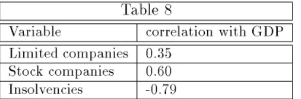
The process of rms' entry and exit takes on an important role in the present model. I shall present some evidence on the behavior of rms' entry and exit decisions over the business cycle. The procyclical behavior of net business formation is well documented for the U.S. economy (see for example Audretsch and Acs, 1991). The following Table reports the contemporaneous correlation of German GDP and three measures of rms' participation rate.

Deviations from the trend of Hodrick-Prescott ltered time series are reported.

Table 8

Variable correlation with GDP Limited companies 0.35

Stock companies 0.60 Insolvencies -0.79

Annual data was logged and Hodrick-Prescott ltered. The variables are the following.

Number of rms: limited companies (GmbHs), stock companies (AGs) and insolvencies.

Basic source of data: Statistisches Bundesamt.

Table 8 reports procyclical behavior of the number of rms in the German economy. In addition, market exit (as measured by insolvency) appears to be present mainly at business cycle downturns.

6.2 Model moments

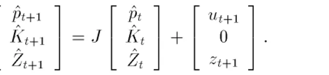
Sunspot equilibria are dened as rational expectations equilibria in which cyclical behavior arises in response to arbitrary random events that do not

(23)

Animal Spirits, Technology Shocks and the Business Cycle 23 have an eect on the fundamental equilibrium conditions of the economy.

Once the sequence of sunspots is generated, the law of motion of the economy, which includes technology shocks, is given by

2

4

^

p

^t+1 K

^t+1 Z

t+1 3

5=^J

2

4

^

p

^t K

^t Z

t 3

5+

2

4 u

t+10

z

t+1 3

5

: (44)

In the remainder of this section I will report the sample moments of my model for various calibrations. The model statistics are computed by applying the formulae developed by Uhlig (1995) on the matrix-valued law of motion (44).²⁴ I will rst specify a baseline calibration which will not be altered unless otherwise noted:

Table 9: Parameters

1⁼ 1⁼

1.00 1.33 1.36 1.03 0.99 0.00

The value of implies that the intraperiod utility is equivalent to that in the Hansen-Rogerson model. The and calibrations follow the notion that signicant increasing returns are only present in the investment goods sector.²⁵ The specic value of is taken from Basu and Fernald (1996).²⁶ I will begin with a version of the model which is driven by a white noise animal spirits shock sequence only.

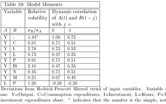
Table 10 considers the case of an economy which is driven by both animal spirits and technology shocks. The volatilities of both of the shocks is set at

z = ^a = 0^:0096.²⁷ Both shocks are uncorrelated. Furthermore I will

24See also the Appendix.

25See the Appendix for a formal derivation of a measure of scale economies in the present model.

26The value is at the upper end of their point estimates.

27McGrattan (1994) drives her version of a standard Real Business Cycle model with a technology shock of^z= 0^:0096. She traces her number from the familiar Solow decom- position by assuming constant returns to scale. No such theoretical counterpart exists to evaluate the variance of the animal spirits shock, however. Farmer and Guo (1994) choose the standard deviation of the animal spirits shock so that the model economy generates times series that match the volatility of U.S. output. As for the animal spirits model, this procedure is perfectly acceptable since no restrictions from the theory apply to the size of