SFB 649 Discussion Paper 2008-031
Beyond the business cycle – factors driving
aggregate mortality rates
Katja Hanewald*
* Humboldt-Universität zu Berlin, Germany
This research was supported by the Deutsche
Forschungsgemeinschaft through the SFB 649 "Economic Risk".
http://sfb649.wiwi.hu-berlin.de ISSN 1860-5664
SFB 649, Humboldt-Universität zu Berlin Spandauer Straße 1, D-10178 Berlin
S FB
6 4 9
E C O N O M I C
R I S K
B E R L I N
Beyond the business cycle - factors driving aggregate mortality rates
Katja Hanewald† 4 April 2008
Abstract
This article provides a comprehensive econometric analysis of factors driving aggregate mortality rates over time. It differs from previous studies in this field by simultaneously considering an extensive set of macroeconomic, socio-economic and ecological factors as explanatory variables. Germany is chosen as an indicative example for other industrialized countries due to its advanced demographic transition process. Our regression analysis, which covers the time interval 1956-2004, indicates that sex- and age-specific mortality rates vary substantially in their response to external factors. Strongest associations are found with changes in real GDP, flu epidemics and the two life style variables alcohol and cigarette consumption in both univariate and multivariate setups. Further analysis shows that these effects are primarily contemporary, while other indicators such as weather conditions exert lagged effects. By combining variables in a multivariate model the share of explained data volatility can be substantially increased. Keywords: Aggregate mortality, business cycle, socio-economic factors, multivariate model. JEL classification: I12, J11, C32.
Introduction
Understanding the development of aggregate mortality rates is not only of crucial importance to social scientists and policymakers concerned with public health, but also to insurance economists. Today, life insurance companies face an increasing demand for funded pension schemes since public pay-as-you-go schemes in most industrialized countries are in the long
† The author is grateful for the support of the German Science Foundation (DFG) and of the Collaborative Research Centre SFB 649. The paper benefited from very helpful comments and suggestions by Tian Zhou- Richter, Helmut Gründl and Thomas Post. Gökce Kirca and Yiran Zhang provided valuable research assistance.
Address: Dr. Wolfgang Schieren Chair for Insurance and Risk Management, Humboldt-Universität zu Berlin, School of Business and Economics, Spandauer Straße 1, 10178 Berlin. Email: katja.hanewald@wiwi.hu- berlin.de.
run unable to cover their obligations due to the demographic transition (see, e.g., Börsch- Supan & Winter, 2001). To allocate sufficient funds and implement adequate risk management strategies, insurance companies need to make assumptions concerning the development of future mortality rates. Unexpected changes in aggregate mortality rates have the potential to cause insolvency of single annuity providers. As systematic risk faced by all life insurance companies, they furthermore pose a very critical threat to future old-age provision and the stability of capital markets in general.
The objective of this research paper is to identify factors driving aggregate mortality rates over time which enable us to predict mortality rates better. In contrast to previous contributions, we provide a comprehensive approach by studying an extensive set of macroeconomic, socio-economic or ecological variables in a multivariate setup. The analysis is based on German data since Germany is by far the most populous country in the European Union. It is, furthermore, among the countries with the most advanced population aging process and can therefore serve as an indicator for future developments in other countries.
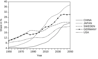
This fact is illustrated in Fig. 1, which depicts UN estimates of the share of the population aged 65 and older. This share is expected to increase in all selected countries, with highest rates occurring in Japan. For the year 2010, the estimates amount to 20.5 percent for Germany and 12.8 percent for the United States. It is expected to reach 20.5 percent in the United States and 30.3 percent in Germany by 2040.
4 8 12 16 20 24 28 32 36 40
CHINA JAPAN SWEDEN GERMANY USA
1950 1970 1990 2010 2030 2050
Share in %
Year
Fig. 1 Share of the population aged 65+, Data from the UN Population Database (medium variant), 2007.
The paper is organized as follows. First, relevant studies on determinants of the mortality process are reviewed systematically. As a fundamental prerequisite for the regression analysis, important characteristics of mortality rates and optimal ways to account for them are discussed next. Then, sources and necessary transformations of the independent variables are summarized and results of the univariate setup are presented. Results are afterwards checked for lagged effects. Finally, we derive three multivariate specifications and compare them.
Challenging points of the analysis are addressed in the discussion part, whereas the conclusion provides a summary and addresses remaining questions.
Literature review
A number of previous studies analyze the effect of single external factors on aggregate mortality rates, i.e. on the rate of deaths occurring in a defined population during a selected time interval. The following section summarizes the related literature for each factor.
A large branch of the epidemiological literature relates fluctuations in mortality rates to macroeconomic factors. In several studies, Brenner (e.g., Brenner, 1973, and Brenner, 1995) found that health decreases and mortality increases during recessions, but his results are often criticized for methodological problems and could not be replicated for other countries or time
periods. On the contrary, Ruhm (2000) discovered a pro-cyclical behavior of mortality rates in the United States using panel data analysis. This rather counterintuitive result implies that more people die when the economy grows faster. The same pattern was found by Tapia Granados (2002, 2003 and 2005a) for mortality rates in Spain, Sweden and the United States, and by Gerdtham & Ruhm (2006) for 23 OECD countries. Furthermore, Neumayer (2004) corroborates Ruhm’s results using data for Germany over the period 1980-2000. He also provides a concise summary of the theories explaining possible positive and negative effects of economic fluctuations on health conditions.
Neumayer stresses the importance of using a fixed effects panel estimator as introduced by Ruhm (2000) to avoid an estimation bias resulting from omitted time-invariant variables1. He argues that this can explain the deviation from Brenner’s results. To apply this estimation method all variables need to be available as time series for different geographical entities, for example for all federal states of Germany as in Neumayer (2004). Yet, Tapia Granados (2005a) finds, by analyzing aggregate mortality rates for the whole USA over the period of 1900-1996, that economic expansions are associated with increasing mortality, which is in line with the results of Ruhm (2000). He uses the following variables to describe the business cycle: unemployment rates, real GDP, an index of manufacturing production, and average weekly hours worked in the manufacturing sector. Of those four, Tapia Granados (2005a) concludes - based on his correlation and univariate regression analysis - that unemployment is the best predictor of fluctuations in mortality rates.
Concerning the relationship between income and mortality rates, two dimensions are generally distinguished in the literature (e.g., see Gravelle, Wildman & Sutton, 2002).
1 Ruhm (2005) points out that location-specific fixed effect regressions should “be viewed complementary rather than as substitutes for time series approach of Tapia Granados and others” since national business cycles are absorbed by the general time effect.
According to the absolute income hypothesis, mortality rates are related to average income, whereas the relative income hypothesis assumes a dependency on the distribution of income.
Using data for 75 countries in 1981 and 1989, Gravelle et al. (2002) find a non-linear positive relation between life expectancy and per capita income, while a significant relation with the Gini coefficient measuring income inequality, could not be detected. This result contradicts a large number of studies that support the relative income hypothesis. However, Gravelle et al.
(2002) vindicate their results by pointing at the problem of aggregating the nonlinear relationship between individual health and income. As a consequence, a positive relationship between population mortality and income inequality can be observed when aggregate data is used, although a causal effect does exist on the individual level. A recent cross-country study by Leigh & Jencks (2007) confirms the result that the effect of income inequality on mortality is statistically insignificant.
Instead of analyzing general macroeconomic indicators, other studies focus on the more direct effect of improvements in the health care system on mortality rates. Felder (2006) finds a positive correlation between public health expenditures as a share of national income and life expectancy in 22 OECD countries for the time period 1970-2003. Nolte & McKee (2003) rank developed countries according to a measure called “mortality amenable to health care”.
Applying a similar concept, Nolte, Scholtz, Shkolnikov, & McKee (2002) discover that the transformation of the East German health system paid a significant contribution to the improvement of life expectancy in East Germany after the German reunification.
A further potential factor driving aggregate mortality rates is weather. Using monthly data for Hong Kong for the period 1980-1994, Yan (2000) detects a significant negative association between cold weather and mortality rates of elderly. Deschenes & Moretti (2007) find that both extreme heat and extreme cold increase U.S. mortality rates immediately. In the case of
cold weather, the increase in mortality exhibits certain persistence and therefore the aggregated effect is larger.
Additionally, several studies account for the fact that some variables exert long delayed effects on health and mortality. For example, Van den Berg, Lindeboom, & Portrait (2006) study the effect of macroeconomic conditions at birth and during childhood on individual mortality rates for cohorts born in the Netherlands during the period 1812 -1912. They find that “the state of the business cycle at birth affects mortality later in life”. Stallard (2006) furthermore points at obesity during childhood development and early adult life. However, lags of 50-75 years would have to be taken into account, which is difficult to realize in the face of actual data availability.
Research design Dependent variables
Since our main objective is to explain what drives aggregate mortality rates over time, age- and sex-specific all-cause mortality rates are the dependent variables in our analysis.
Corresponding data for Germany was retrieved from the Human Mortality Database (HMD), which provides standardized data for a large number of countries. According to Wilmoth, Andreev, Jdanov, & Glei (2007), these mortality rates were calculated by dividing death counts by estimates of the population exposed to the risk of death in the same intervals of age and time.
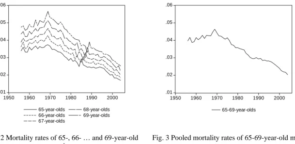
Our analysis is based on 5-year age groups for the following reasons. Studying one-year-age- group mortality rates, an astonishing volatility pattern was found, which is shown exemplarily for 65- to 69-year-old males in Fig. 2. Mortality rates of 65- year-old males increase in volatility at the beginning of the 1980s when two smaller peaks in the series are followed by a
sharp increase in 1985. For 66-year-olds this pattern is shifted forward by one year, for 67- year-olds by two years. Mortality rates of 75-year-olds are shocked in a similar way in 1995.
The pattern exists for females as well and can be observed for all 40- to 80-year-old individuals. This observation made us question the quality of data provided by the Human Mortality Database. Using death counts and population data from the German Federal Statistical Office, we constructed a crude rate for comparison. The resulting graphs exhibit volatility patterns similar to those found in corresponding data from the Human Mortality Database.
.01 .02 .03 .04 .05 .06
1950 1960 1970 1980 1990 2000
65-year-olds 66-year-olds 67-year-olds
68-year-olds 69-year-olds
.01 .02 .03 .04 .05 .06
1950 1960 1970 1980 1990 2000
65-69-year-olds
Fig. 2 Mortality rates of 65-, 66- … and 69-year-old males
Fig. 3 Pooled mortality rates of 65-69-year-old males
The obvious question concerns the origin of the observed pattern. The fact that it is always shifted by one year for consecutive age groups suggests that it is caused by a cohort effect rather than by a time effect related to the year of death. One common characteristic of the affected age groups is that they were born at the end or shortly after the First World War. As a consequence of the Allied blockade of Germany which began in 1915 and officially continued until July 1919, this period was characterized by a shortage of food supply that persisted till 1920 (see e.g. Horiuchi, 1983). According to data cited by Birrer (2004), the average daily consumption of calories in Germany dropped from 3,280 in 1912-13 to 1,456 in August 1919.
The observed mortality increase is likely to be a late effect of this hunger period, as Van den Berg, Lindeboom & Portrait (2006) point out that the detrimental effect of malnutrition of the
mother at the end of pregnancy on the morbidity of her child after the age of 50 is well established through empirical findings. Furthermore, German males born in 1919 or 1920 were among the first to be drafted for military services in World War II since most of them were still doing their two years of military service at the outbreak of war in September 1939.
They experienced the war’s hardships in full length with potentially adverse consequences for their later health.
As a solution, we decided to pool the population to 5-year age groups which deletes the observed cohort effect2, as one can see from Fig. 3. For the further analysis, the age groups of 25-29-, 35-39- … 95-99-year-olds have been selected.
In Fig. 4 mortality rates of 65-69-year-olds are plotted for both sexes. Over the whole sample period mortality rates of males are higher than those of females, indicating that females die on average at higher ages. Furthermore, a downward trend can be detected in both series which translates into an increased life expectancy. Applying the augmented Dickey-Fuller test confirms that both series are non-stationary. This is the case for mortality rates of all 5-year- age groups and for a large number of independent variables included in the analysis. To avoid spurious regressions, non-stationary variables are transformed into relative changes by taking the first difference of the logarithmized series3.
2 On the other hand, pooling data also deletes information. Alternatively, one could include an independent variable measuring average calories per person per day in the year of birth to control for malnutrition.
3Applying the first difference directly, i.e. analyzing absolute changes would have the same effect. However, relative changes are more convenient to interpret since they indicate yearly percentage changes.
.00 .01 .02 .03 .04 .05
1950 1960 1970 1980 1990 2000
Males Females
Fig. 4 Mortality rates of 65-69-year-olds.
-.12 -.08 -.04 .00 .04 .08
1950 1960 1970 1980 1990 2000
Males Females
Fig. 5 Mortality rates of 65-69-year-olds, relative changes.
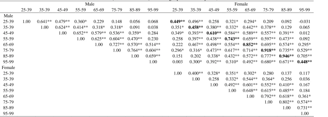
In a next step, we compare yearly changes in age-specific mortality rates of males and females. Table 1 displays the corresponding correlation coefficients; those between males and females at the same age interval are plotted in bold font. For 25-29-year-olds this correlation amounts to 44.9 percent, it increases with age up to 94.6 percent for 85-89-years-olds, but drops for 95-99-years-olds to 44.8 percent. Studying neighboring age groups, e.g. 45-49- and 55-59-year-olds, we find that the average correlation amounts to 67 percent for males and to 59 percent for females. These observations corroborate that mortality rates should be analyzed separately for the two sexes and different age groups.
The sample
The whole period 1956-2004, for which German data is available in the HMD, is included in the analysis. This time span covers the German reunification in 1990. We set the convention that data until 1990 describes West Germany, while from 1991 onwards all series correspond to whole Germany. This approach is necessary since data for East Germany before 1991 is scarcely available and the majority of time series provided by the German Federal Statistical Office does not distinguish between East and West Germany anymore for recent data.
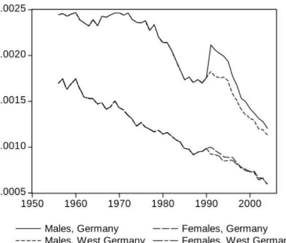
Since the beginning of the 1970s mortality rates in West Germany decreased substantially faster than in East Germany. Luy (2006) documents that the resulting differential in life expectancies at birth between West and East Germany topped in 1988 for women at 2.95 years and in 1990 for men at 3.54 years. In accordance to this, we see an increase in aggregate mortality rates when East Germany is added to the sample4. The effect is larger for males and for younger age groups. It is largest for mortality rates of 35-year-olds which are exemplarily shown in Fig. 6. Apparently, the increase in German mortality rates at the beginning of the 1990s is not only due to the inclusion of East Germany, since mortality has also increased in the Western part5. Other age groups exhibit a similar pattern. In the long run, a permanent shift in the level of mortality rates cannot be detected. This is in line with Luy (2006) who states that instead of inducing a “mortality crisis”, the reunification caused a rapid decline in excess mortality in East Germany. Fig. 7 displays the series of relative changes in the mortality rates of 35-39-year-old males. The change in the sample due to the reunification translates into a peak in 1991. Therefore, a dummy variable is appropriate to account for this effect in the regression analysis.
4 In 1990, the population of West and East Germany amounted to 64 and 16 million, respectively.
5 This effect is possibly due to inner-German migration. In 1989-90, for example, 785,000 individuals left East Germany, most of them heading for West Germany.
.0005 .0010 .0015 .0020 .0025
1950 1960 1970 1980 1990 2000
Males, Germany Males, West Germany
Females, Germany Females, West Germany
Fig. 6 Mortality rates of 35-39-year-olds.
-.10 -.05 .00 .05 .10 .15 .20
1950 1960 1970 1980 1990 2000
Males, Germany Males, West Germany
Fig. 7 Mortality rates of 35-39-year-old males, relative changes.
Independent variables
The literature review showed that a number of studies exist focusing on selected factors influencing aggregate mortality rates. To provide a comprehensive analysis, we include all variables mentioned earlier, as well as important additional potential factors such as long run unemployment rates or the average actual retirement age. The following section gives an overview of the independent variables, their sources and transformations.
Real GDP time series provided by the German Federal Statistical Office suffer from a methodological break in 1970. Alternatively, Angus Maddison’s widely cited Historical Tables could be used. However, his series are backward projections for today’s national borders which implies that East Germany’s GDP is included in the German GDP even before 1990. A series for West Germany only until 1990 and for whole Germany from 1991 on was obtained from the Total Economy Database by the Conference Board and Groningen Growth and Development Centre.
Unemployment rates were obtained from the Institute for Employment Research (IAB), while long-term unemployment rates for 1977-1999 were received from the statistics
department of Germany’s federal employment services. From 2000 on, long-term unemployment rates had to be constructed with data from the German Federal Statistical Office. The latter also provided employment rates which measure the share of gainfully employed persons in the total population aged 15-65. Data on average hours worked were obtained from the German Federal Statistical Office, too. It contains the actual average numbers of hours worked in the predominant occupation per gainfully employed person during the reference week. In this average, working hours of civil servants as well as those of self-employed are included. A series on average actual retirement age was obtained from the German Pension Fund. All labor market variables except long-term unemployment rates enter the regression as sex-specific indicators.
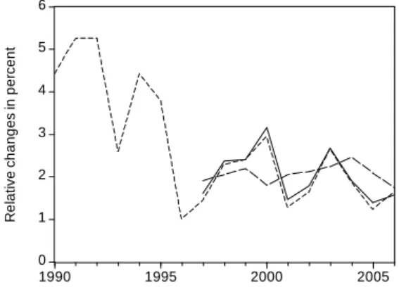
Data on average gross monthly earnings in the manufacturing sector provided by the German Federal Statistical Office is only available for whole Germany from 1996 on. We tried to solve this problem by using growth rates of earnings in West Germany to construct the missing values for whole Germany for 1991-1995. Fig. 8 confirms that yearly changes in gross monthly earnings of the whole country are mainly induced by those of West Germany.
0 1 2 3 4 5 6
1990 1995 2000 2005
Germany West Germany East Germany
Relative changes in percent
Fig. 8 Relative changes in gross monthly earnings in the manufacturing sector.
Another source of private households’ income are capital market investments. Therefore, we include the DAX index into the set of possible regressors. This blue chip index lists the top 30 largest German companies in terms of order book volume and market capitalization and was introduced in 1988; Stehle (2008) provides a backward projection of yearly real returns until 1948. Furthermore, we include the Ifo Index which is an early indicator for the cyclical development of the German economy provided by the Institute for Economic Research (Ifo).
It is based on a monthly survey conducted in 7,000 companies. Series are available for 1969- 2005 for West Germany and from 1991 on for unified Germany. We chose the series „Ifo Business climate, R3, Trade and industry business expectations“, which summarizes expectations of the business climate in the next six months.
Apart from wages and capital income, households also receive social benefits such as child allowance, unemployment benefits or pension payments. A series on “Social benefits per capita in Euro” can be found in the report “Social Budget 2006” published by the German Federal Ministry of Labor and Social Affairs (BMAS). The data is available from 1960 on.
Public health expenditures at the 2000 GDP prices were obtained from the OECD Health Database 20066 where they are available for 1970-2003 with a missing value in 1991, which we imputed by an average of the values for 1990 and 1992.
As an indicator of the cost of living, inflation given by the growth rate of the consumer price index is included into the analysis. The series was constructed using data published in the Statistical Yearbook 2004 and 2007 by the German Federal Statistical Office.
Besides, daily average temperatures of up to 13 weather stations that are well distributed over Germany were retrieved from the database of the Deutscher Wetterdienst (DWD)7 to create an
6 It is the best available data set since the German Federal Statistical Office offers real per capita health expenditures only from 1992 on and nominal values for 1970-1998.
7 We are indebted to the Financial and Economic Data Center (FEDC) of the Collaborative Research Center (SFB) 649 at the Humboldt University of Berlin for an access to DWD data.
average daily temperature for the whole country. Four different variables were constructed from this data set. They contain the number of days per year below 0°C, -5°C and -10°C, as well as the number of days with an average temperature above 25°C8.
Furthermore, it will be analyzed to what extent aggregate mortality rates are affected by flu epidemics. Therefore, a variable containing the number of influenza and pneumonia deaths as a standardized rate per 100,000 of the population is added to the set of regressors. The data was taken from the OECD Health Database 2006 where it is available for 1960-2004.
Time series on cigarette and spirits consumption in Germany from 1952 on were obtained from the German Federal Statistical Office. Cigarette consumption is counted in cigarettes per potential consumer, which refers to the population age 15 and older. Spirits consumption is given in liters per potential consumer using the same age interval. Both series have a missing value in 1990 which was imputed by an average of the values for 1989 and 1991. Time series related to nutrition were found in the OECD Health Database 2006. “Calories per capita per day” and “Total fat intake” measured in grams per capita per day were chosen. Both time series are available for 1961-2003.
Univariate Regressions Estimation technique
We follow the approach of Tapia Granados (2005a) by regressing relative changes in mortality rates on an intercept β0 and on one economic or ecological factor Xt. Additionally, we include a dummy variable DUM indicating the years 1991 and 1992 to account for the German reunification. The econometric specification is summarized by the following equation:
0 1 2
ln(MRt) β βDUM β ln(Xt) et
Δ = + + Δ + ,
8 Over the whole sample period, the highest daily average temperature was measured on August 9, 1992 with 28.02°C; the minimum occurred on February 1, 1956 with -17.66°C.
where MRt are age- and sex-specific mortality rates. All of the independent variables Xt are transformed to relative changes, except real Dax returns, inflation and the number of cold or hot days. In case of the variable “average actual retirement age” the regression setup is also altered by allowing for lagged effects. Over the sample period, the mean value of this variable is 60 years for males and 61 years for females. It is therefore only included into the regression equations for elderly with the following lags: no lag for 65-69-year-olds, 10 years lag for 75- 79-years olds,…, and 30 years lag for 95-99-years-olds.
Results
Regression results are summarized in Table 2 and Table 3 and the threshold for significant p- Values is set to 0.05 percent in the following analysis. First, real GDP growth rate is a significant regressor for changes in mortality rates of males aged 25-29 to 65-69, as well as for females aged 25-29 to 55-59. In all cases the effect is positive, which is in line with Ruhm (2000) and Granados (2005a), who found that mortality increases when GDP grows faster.
However, in contrast to Granados (2005a) our results do not indicate a stronger relationship of mortality with unemployment rates than with GDP; only for 55-59-year-old males and females a significant negative relationship between unemployment rates and mortality can be detected. Furthermore, a significant positive association between employment rates is observed for males aged 35-39 and 55-59, as well as for 35-39-year-old females.
In case of the other variables capturing labor market conditions - long-term unemployment rates, hours worked, and average actual retirement age - no significant regressors were found.
The same holds true for the two business indicators DAX returns and Ifo Index, as well as for social benefits and health expenditures. Similarly, changes in the consumer price index measured by the variable inflation have no impact on aggregate mortality rates. Estimated effects on relative changes in aggregate mortality rates caused by the number of days with
extreme temperatures are also very small. Only for 55-59-year-old males and 25-29-year-old females both coefficients on the number of days below -5°C and below -10°C are significant.
In contrast to that, we find that flue epidemics affect aggregate mortality rates considerably.
The observed effects strongly increase with age. For males, all estimated coefficients on changes in the number of influenza and pneumonia deaths from the age 65-69 onwards are significant, for females this is the case from 55-59 years on. Up to the age of 55-59 years flu epidemics have a stronger impact on mortality rates of females; beyond that both males and females react similarly. Only for 95-99-year-olds is the estimated coefficient substantially lower for females than for males.
Finally, a number of significant coefficients can be found in the group of “life style” variables.
Significant positive coefficients exist for cigarette consumption in the case of males aged 35- 39 to 65-69 and for females aged 85-89. Spirits consumption, on the other hand, seems to affect higher age groups and females more. It is significantly positively related to mortality rates of males aged 55-59 to 85-89 and of females aged 45-49 to 85-89. For total calories and total fat intake there are no significant effects for any age group.
Lagged effects
Up to now we assumed that mortality rates respond instantaneously to external factors. To account for delayed effects, the analysis was repeated with one-year lagged regressors:
0 1 2 1
ln(MRt) β βDUM β ln(Xt−) et
Δ = + + Δ + .
The corresponding results, which are displayed in Table 4 and Table 5, indicate that changes in GDP do not affect next year’s mortality rates. In case of flu epidemics, alcohol or cigarettes, the number of significant effects also decreased considerably. Apart from that, some other variables gain in importance. For example, mortality rates of 35-39- and 55-59-year-old males
respond to changes in average monthly earnings in the previous year, while this is the case for 45-49-, 65-69- and 75-79-year-old males and social expenditures. Besides, lagged significant relations can be found between the number of days below -5°C and mortality rates of males and females aged 85-89 and 95-99.
Multivariate Regressions
In the following, relative changes in mortality rates will be regressed on multiple economic or ecological factors, an intercept term and a dummy variable indicating the years 1991-92.
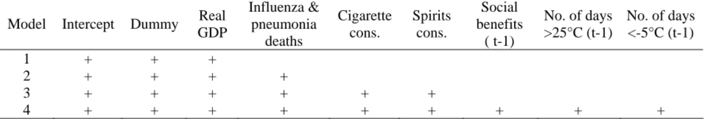
Based on the univariate regression results, three different multivariate specifications are derived; they are summarized in Table 6. As a benchmark, results of the simple regressions on changes in real GDP (Model 1) are included into the comparison. Model 2 contains relative changes in the number of influenza and pneumonia deaths in addition to real GDP. Model 3 furthermore incorporates cigarette and spirits consumption. This set of explanatory variables is again extended in Model 4 by relative changes in the social benefits per capita, as well as by the number of cold and hot days.
Table 6 Variables in multivariate regression models.
Model Intercept Dummy Real GDP
Influenza &
pneumonia deaths
Cigarette cons.
Spirits cons.
Social benefits
( t-1)
No. of days
>25°C (t-1)
No. of days
<-5°C (t-1) 1 + + +
2 + + + +
3 + + + + + +
4 + + + + + + + + +
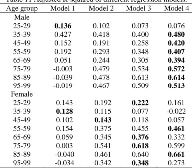
The corresponding results can be found in Table 7-10, where each line represents the estimated coefficients of one regression equation. The models are compared on the basis of the adjusted coefficient of determination R2 , which weighs the goodness of fit of the regression model with the number of regressors. For convenience, the measure is collected in Table 11 and maximal values are indicated with bold font.
Table 11 Adjusted R-squared of different regression models.
Age group Model 1 Model 2 Model 3 Model 4
Male
25-29 0.136 0.102 0.073 0.076
35-39 0.427 0.418 0.400 0.480 45-49 0.152 0.191 0.258 0.420 55-59 0.192 0.293 0.348 0.407 65-69 0.051 0.244 0.305 0.394 75-79 -0.003 0.479 0.534 0.572 85-89 -0.039 0.478 0.613 0.614 95-99 -0.019 0.467 0.509 0.513 Female
25-29 0.143 0.192 0.222 0.161 35-39 0.128 0.115 0.077 -0.022 45-49 0.102 0.143 0.118 0.057 55-59 0.154 0.375 0.455 0.461 65-69 0.059 0.345 0.376 0.332 75-79 0.003 0.541 0.618 0.599 85-89 -0.040 0.461 0.640 0.661 95-99 -0.034 0.342 0.348 0.273
We find that including an indicator for flu epidemics (Model 2) substantially improves Model 1’s ability to explain changes in the mortality rates of males and females aged 45-49 and older.
For the same age groups (except for 45-49-year old females) the model’s explanatory power can further be increased considerably by adding the two life style variables cigarettes and spirits consumption. Even better results can be found by including the three lagged variables.
Model 4 turns out to be optimal according to R2 for changes in the mortality rates of males aged 35-39 and older and for females aged 55-59 and 85-89. For females aged 25-29, 65-69, 75-79 and 95-99, Model 3 is optimal. The benchmark case Model 1 dominates only for 25-29- years-old-males and 35-39-year-old females. If one was to choose one model for all age groups, Model 4 should be selected for males while Model 3 seems favourable for females.
The fit of these multivariate models is substantially better compared to the univariate Model 1 for 14 out of 16 analyzed age groups.
Discussion
At first glance, contemporary effects of cigarette and spirits consumption on aggregate mortality rates are difficult to interpret. According to Rübenach (2007), the most common
alcohol related cause of death in Germany in 2005 was alcoholic cirrhosis of liver followed by the alcohol dependency syndrome which subsumes mental disorders and behavioral disturbances caused by alcohol. Rübenach (2007) points out that both diseases develop as a consequence of continued alcohol abuse. Detrimental effects of smoking on the respiratory and cardiovascular system are of a likewise long-term character.
An alternative explanation could be that the observed effects are confounded by the general economic situation. Neumayer (2004) mentions that increases in income during economic expansions may result in higher consumption of cigarettes and alcohol. Indeed, positive correlations between changes in real GDP growth rates and changes in the consumption of the two luxury goods can be detected. Over the time interval 1956-2004 9the correlation coefficient between GDP and cigarette consumption amounts to 0.572, while it is 0.423 for spirits consumption10. These relations are reflected in the estimated regression coefficients as well. Significant effects on mortality rates of males aged 35-39 to 65-69 were found in the univariate analysis both for real GDP and cigarette consumption. However, for females the effects do not overlap. In the case of spirits consumption, significant effects are estimated especially for higher age groups up to the age 85-89 for males and females, whereas fluctuations in the domestic product only affect the working age population. These considerations suggest accepting changes in spirits consumption as an independent factor driving aggregate mortality rates but treating effects of cigarette consumption with caution.
Furthermore, the small number of significant effects in the group of the macroeconomic variables is to some extent surprising. Yet, many time series possibly influencing the level of mortality rates such as average hours worked per week or public health expenditures are too
9 In accordance with the dummy included in the regression analysis, the years 1991 and 1992 are excluded.
10 The correlation between changes in alcohol and cigarette consumption amounts to 0.343.
smooth to explain yearly changes. However, analyzing variables in levels carries the risk of spuriously regressing time trends on each other.
Conclusion
The objective of this research paper is to identify factors driving aggregate mortality rates in Germany. Based on the descriptive analysis at the beginning of the study, relative changes in aggregate mortality rates are analyzed separately for males and females and for different age groups. The extensive set of explanatory variables includes major factors known from the epidemiological literature as well as additional factors. Result of the univariate regression analysis suggest that growth rates of real GDP are positively related with mortality rates of working-age males and females which is in line with number of recent studies. Beyond that, we find that flu epidemics significantly affect mortality rates of higher age groups. Moreover, our results indicate that changes in alcohol consumption are positively associated with aggregate mortality rates of males and females aged 55-59 to 85-89 and aged 45-49 to 85-89 respectively. For cigarette consumption this is the case for mortality rates of 35-39- to 55-59- year-old males. A replication of the analysis with lagged effects shows that the above- mentioned effects are primarily contemporary, while other variables such as changes in social benefits or the number of cold and hot days exert lagged effects. In a next step, we combined the identified variables and compared three plausible multivariate specifications. The resulting models are able to explain up to 66 percent of the volatility in the observed mortality rates and thereby confirm the relevance of the identified factors.
While our study focuses on yearly changes in mortality rates, the question of long-run causes of mortality improvements in industrialized countries remains open. Brenner (2005) claims that economic growth was the main driver of mortality decline in the 20th century. Tapia Granados (2005b), on the other hand, states that there is no causal connection between these
two variables and that only two time trends coincide. Obviously, in industrialized countries such as Germany further improvements in the standard of life or in primary health care only play a minor part. Significant upward shifts in the life expectancy can therefore only be expected as a result of major medical or technical innovations which a large share of the population can access. With the advance of luxury diseases such as obesity or alcohol addiction, however, aggregate mortality rates might potentially rise again in the near future.
References
Börsch-Supan, A., & Winter, J. (2001). Population Ageing, Savings Behavior and Capital Markets. NBER Working Paper Series, 8561.
Birrer, C. (2004). A Critical Analysis of the Allied Blockade of Germany, 1914-1918. Journal of the Centre for First World War Studies, 1, 35-67.
Brenner, M. H. (1973). Mental illness and the economy. Cambridge: Harvard University Press.
Brenner, M. H. (1995). Political economy and health. In Benjamin, C.A., Levine, S., Tarlov, A.R. and Walsh, D.C. (Ed.), Society and Health (pp. 211–246). Oxford: Oxford University Press.
Brenner, M. H. (2005). Commentary: Economic growth is the basis of mortality rate decline in the 20th century—experience of the United States 1901–2000. International Journal of Epidemiology, 34, 1214–1221.
Deschenes, O., & Moretti, E. (2007). Extreme weather events, mortality and migration. NBER Working Paper Series, 13227.
Felder, S. (2006). Lebenserwartung, medizinischer Fortschritt und Gesundheitsausgaben:
Theorie und Empirie. Perspektiven der Wirtschaftspolitik. 7 (Special issue), 49–73.
Gerdtham, U.G., & Ruhm, C. J. (2006). Deaths rise in good economic times: Evidence from the OECD. Economics & Human Biology, 4, 298-316.
Gravelle, H., Wildman, J., & Sutton, M. (2002). Income inequality, and health: what can we learn from aggregate data. Social Science & Medicine, 54, 577–589.
Horiuchi, S. (1983), The long-term impact of war on mortality: old-age mortality of the First World War survivors in the Federal Republic of Germany, Population Bulletin of U.N., 15, 80-92.
Leigh, A. & Jencks, C. (2007). Inequality and mortality: Long-run evidence from a panel of countries. Journal of Health Economics, 26, 1–24.
Luy, M. (2006). Differentielle Sterblichkeit: die ungleiche Verteilung der Lebenserwartung in Deutschland. Rostocker Zentrum–Diskussionspapier, No. 6.
Maddison, A. (2007). World Population, GDP and per capita GDP, 1-2003 AD.
Neumayer, E. (2004). Recessions lower (some) mortality rates: Evidence from Germany.
Social Science & Medicine. 58, 1037–1047.
Nolte, E., & McKee, M. (2003). Measuring the health of nations: analysis of mortality amenable to health care. British Medical Journal. 327, 1129-32.
Nolte, E., Scholtz, R., Shkolnikov, V., & McKee, M. (2002). The contribution of medical care to changing life expectancy in Germany and Poland. Social Science & Medicine. 55, 1905–21.
Van den Berg, G. J., Lindeboom, M., & Portrait, F. R. M. (2006). Economic Conditions Early in Life and Individual Mortality. American Economic Review. 96, 290-302.
nach, S. P. (2007). Die Erfassung alkoholbedingter Sterbefälle in der Todesursachenstatistik 1980 bis 2005. Wirtschaft und Statistik. 3, 270-290.
Zu viele Leerzeichen, irgendwie könnte ich sie nicht löschen.
Ruhm, C. J. (2005). Commentary: Mortality increases during economic upturns. International Journal of Epidemiology, 34, 1206–1211.
Ruhm, C. J. (2000). Are Recessions Good for Your Health?. The Quarterly Journal of Economic, 115, 617-650.
Stallard, E. (2006). Demographic Issues in Longevity Risk Analysis. Journal of Risk &
Insurance, 73, 575–609.
Statistisches Bundesamt (2004). Statistisches Jahrbuch 2004 für die Bundesrepublik Deutschland und das Ausland. Stuttgart: Metzler-Poeschel.
Statistisches Bundesamt (2007). Statistisches Jahrbuch 2007 für die Bundesrepublik Deutschland und das Ausland. Stuttgart: Metzler-Poeschel.
Stehle, R. (2008). Jährliche reale Renditen deutscher Blue-Chip-Aktien 1948 bis 2007 (in %).
Institut für Bank-, Börsen- und Versicherungswesen, Humboldt-Universität zu Berlin.
Tapia Granados, J. A. (2002). Mortality and economic fluctuations–Theories and empirical results from Spain and Sweden. PhD Dissertation. Chapter 2. Department of Economics, Graduate Faculty of Political and Social Science, New School University, New York.
Tapia Granados, J. A. (2003). Mortality and economic fluctuations in Sweden, 1800-1998.
Paper presented at the 2004 Meeting of the Population Association of America. Boston, MA .
Tapia Granados, J. A. (2005a). Increasing mortality during the expansion of the U.S. economy 1900-1996. International Journal of Epidemiology, 34, 1194-1202.
Tapia Granados, J. A. (2005b). Response—on economic growth, business fluctuations, and health progress. International Journal of Epidemiology, 34, 1226–1233.
The Conference Board and Groningen Growth and Development Centre (2007). Total Economy Database. http://www.ggdc.net, data downloaded on November 11, 2007.
United Nations Population Division (2007). World population prospects: population database, 2006 revision. http://esa.un.org/unpp, data downloaded on Feb 26, 2008.
University of California, Berkeley, USA & Max Planck Institute for Demographic Research, Germany (2007). Human Mortality Database. http://www.mortality.org/, data downloaded on November 1, 2007.
Van den Berg, G. J., & Lindeboom, M. & Portrait, F. R. M. (2006). Economic Conditions Early in Life and Individual Mortality. American Economic Review. 96, 290-302.
Wilmoth, J. R., Andreev, K., Jdanov, D., & Glei, D.A. (2007). Methods Protocol for the Human Mortality Database. Version 5.
Yan, Y. Y. (2000). The influence of weather on human mortality in Hong Kong. Social Science & Medicine. 50, 419–427.
Table 1 Correlations (Pearson coefficient) between age-specific mortality rates, 1956-2004.
Male Female
25-39 35-39 45-49 55-59 65-69 75-79 85-89 95-99 25-39 35-39 45-49 55-59 65-69 75-79 85-89 95-99 Male
25-39 1.00 0.641** 0.479** 0.360* 0.229 0.148 0.056 0.068 0.449** 0.496** 0.258 0.321* 0.294* 0.209 0.092 -0.031 35-39 1.00 0.624** 0.414** 0.318* 0.318* 0.091 0.038 0.351* 0.458** 0.380** 0.332* 0.442** 0.378** 0.129 0.065 45-49 1.00 0.652** 0.579** 0.536** 0.359* 0.284 0.349* 0.393** 0.610** 0.584** 0.589** 0.557** 0.391** 0.012 55-59 1.00 0.625** 0.604** 0.470** 0.230 0.258 0.397** 0.438** 0.743** 0.659** 0.597** 0.473** 0.092 65-69 1.00 0.727** 0.570** 0.514** 0.222 0.467** 0.498** 0.554** 0.852** 0.695** 0.574** 0.295*
75-79 1.00 0.764** 0.604** 0.296* 0.316* 0.473** 0.617** 0.714** 0.918** 0.735** 0.529**
85-89 1.00 0.659** 0.151 0.202 0.338* 0.432** 0.572** 0.777** 0.946** 0.705**
95-99 1.00 0.003 0.300* 0.392** 0.310* 0.492** 0.680** 0.671** 0.448**
Female
25-39 1.00 0.400** 0.328* 0.351* 0.302* 0.280 0.137 0.117 35-39 1.00 0.258 0.332* 0.544** 0.364* 0.256 0.036 45-49 1.00 0.492** 0.601** 0.552** 0.410** 0.167
55-59 1.00 0.648** 0.615** 0.485** 0.184
65-69 1.00 0.792** 0.618** 0.361*
75-79 1.00 0.802** 0.574**
85-89 1.00 0.731**
95-99 1.00
Mortality rates are transformed to relative changes. * P<0.05, ** P<0.01 (2-tailed).
Table 2 Univariate regressions, mortality rates as dependent variables, estimated coefficients.
Age group Real GDP Unemployment rate1)
Long –term unemployment rate
Employment rate1)
Hours worked1)
Retirement age1)
Monthly earnings
DAX
returns Ifo Index Social benefits
Male
25-29 0.705* -0.019 -0.041 1.228 -0.744 0.191 0.008 0.335 -0.013 35-39 0.818** -0.011 -0.048 1.213* -0.500 0.279 -0.006 0.020 0.101 45-49 0.417* -0.009 -0.035 0.488 -0.629 0.157 0.002 0.028 0.129 55-59 0.390** -0.020* 0.004 0.641* -0.395 0.166 -0.009 -0.016 0.060 65-69 0.385* -0.013 0.003 0.103 -0.694 0.306 0.208 0.013 0.068 0.116 75-79 0.230 -0.002 -0.017 0.312 -0.828 0.310 0.166 0.014 -0.175 0.155 85-89 0.034 0.006 -0.039 0.377 -0.518 0.385 -0.028 0.002 -0.023 0.052 95-99 -0.183 0.003 -0.125 0.270 -0.579 2.579+ -0.293 0.036 -0.082 -0.106
Female
25-29 0.494* -0.006 -0.054 0.358 -0.314 0.239 -0.006 -0.418* 0.112 35-39 0.590** -0.031 -0.068 0.655* -0.263 0.137 0.018 -0.258 0.039 45-49 0.393* -0.026+ -0.062 0.352 0.321 0.027 -0.003 -0.060 -0.066 55-59 0.316** -0.023* -0.004 0.204 0.052 0.054 -0.008 0.014 -0.049 65-69 0.328+ -0.020 0.015 0.173 0.098 -0.052 0.047 0.003 0.000 -0.038 75-79 0.158 -0.012 -0.038 0.293 -0.441 -0.827 -0.012 0.011 -0.115 0.015 85-89 0.087 -0.020 -0.056 0.363 -0.381 -0.996 -0.064 -0.003 -0.008 -0.014 95-99 0.047 -0.015 0.026 0.314 -1.228* 2.899 -0.118 0.016 -0.002 -0.079 Sample Period 1957-2004 1957-2004 1978-2003 1958-2004 1958-2004 1961-2004 1957-2004 1967-2004 1992-2004 1961-2004
All variables are transformed to relative changes except DAX returns. 1) sex-specific independent variable. + P<0.1, * P<0.05, ** P<0.01.
Table 3 Univariate regressions, mortality rates as dependent variables, estimated coefficients.
Age group Health
expenditures Inflation No. of days
>25°C
No. of days
< -5°C
No. of days
< -10°C
Influenza &
pneumonia deaths
Cigarette consumption
Spirits consumption
Total calories
Total fat intake Male
25-29 0.119 -0.247 0.004 0.001 0.000 -0.001 0.138 0.031 -0.898+ -0.447
35-39 0.322+ 0.152 -0.001 0.000 -0.002 0.001 0.245* 0.084 0.189 0.309 45-49 0.231+ 0.075 -0.001 0.000 0.000 0.017 0.203** 0.089+ -0.188 0.274 55-59 0.074 -0.020 -0.001 0.001* 0.003* 0.022 0.153** 0.100** -0.044 0.100 65-69 0.017 0.037 0.000 0.001 0.002 0.061** 0.200* 0.120* -0.368 -0.098 75-79 0.139 0.260 -0.005* 0.001 0.002 0.095** 0.121 0.149** -0.252 -0.027 85-89 0.073 0.257 -0.004 0.001 0.003 0.143** 0.187 0.166* -0.395 0.511 95-99 -0.004 0.025 -0.003 0.001 0.002 0.191** 0.079 0.138 -0.650 -0.244 Female
25-29 0.187 0.134 -0.001 -0.001* -0.006* 0.035 -0.038 0.065 -0.310 -0.367 35-39 0.103 -0.025 0.002 0.000 -0.001 0.034 0.146 0.064 -0.489 -0.681+
45-49 0.100 -0.396 -0.003 0.001 0.003 0.034+ 0.107 0.107* -0.038 0.438 55-59 0.004 -0.148 0.000 0.000 0.002 0.032* 0.101+ 0.123** -0.057 0.069 65-69 0.005 -0.020 -0.001 0.001 0.002 0.061** 0.136+ 0.114* -0.209 0.019 75-79 0.051 0.090 -0.004+ 0.001 0.002 0.105** 0.124 0.139* -0.226 0.070 85-89 0.056 0.040 -0.001 0.001 0.003 0.130** 0.233* 0.145* -0.449 0.416 95-99 -0.070 0.019 -0.003 0.000 -0.001 0.116** 0.099 0.131+ -0.179 0.403 Sample
Period 1971-2003 1957-2004 1957-2004 1957-2004 1957-2004 1961-2004 1957-2004 1957-2004 1968-2004 1968-2004 All variables are transformed to relative changes except the number of hot or cold days and inflation. + P<0.1, * P<0.05, ** P<0.01.
Table 4 Univariate regressions, mortality rates as dependent variables, lagged values of independent variables, estimated coefficients.
Age group Real GDP Unemployment rate1)
Long –term unemployment rate
Employment rate1)
Hours worked1)
Retirement age1)
Monthly earnings
Dax
returns Ifo Index Social benefits
Male
25-29 -0.010 -0.028 -0.105 1.806* 0.609 0.426+ -0.033 -0.052 0.230 35-39 0.017 -0.004 -0.079 1.007+ -0.924 0.460* -0.010 -0.000 0.101 45-49 0.014 0.003 -0.042 0.617 -0.909+ 0.261+ -0.009 -0.165+ 0.354**
55-59 0.178 -0.012 -0.004 0.722* 0.087 0.216* 0.000 -0.024 0.141+
65-69 0.200 0.005 -0.041 0.205 -0.407 0.226 0.189 -0.007 -0.047 0.264*
75-79 0.092 0.013 -0.011 0.058 -0.885 -0.203 0.199 -0.006 0.010 0.288*
85-89 -0.077 0.019 -0.076 0.250 -0.163 -0.772 0.017 -0.011 -0.231 0.255 95-99 -0.019 0.030 -0.071 -0.099 -0.882 -0.354 -0.140 0.010 -0.020 0.103
Female
25-29 0.142 -0.003 -0.014 0.152 -0.656 0.263 -0.028 0.217 0.158 35-39 0.104 0.006 -0.048 -0.104 -0.699 0.084 0.008 0.192 0.039 45-49 0.151 -0.015 -0.071 0.276 -0.890* 0.011 0.004 -0.209+ 0.060 55-59 -0.040 0.004 -0.015 -0.111 -0.237 0.002 0.002 -0.018 0.046 65-69 -0.063 0.012 -0.051 -0.204 -0.475 -0.498 0.058 0.001 -0.036 0.140 75-79 -0.003 0.020 -0.069+ -0.208 -0.355 0.211 0.065 -0.005 -0.129 0.177 85-89 -0.050 0.025 -0.088 -0.168 -0.081 -2.137 -0.094 -0.008 -0.188 0.122 95-99 -0.017 0.028 -0.066 -0.221 0.430 -2.812 -0.129 -0.002 -0.157 0.036 Sample
Period 1957-2004 1957-2004 1979-2003 1959-2004 1959-2004 1962-2004 1957-2004 1968-2004 1993-2004 1962-2004 All variables are transformed to relative changes except DAX returns. + P<0.1, * P<0.05, ** P<0.01.
Table 5 Univariate regressions, mortality rates as dependent variables, lagged values of independent variables, estimated coefficients.
Age group Health
expenditures Inflation No. of days
>25°C
No. of days
< -5°C
No. of days
< -10°C
Influenza &
pneumonia deaths
Cigarette consumption
Spirits consumption
Total calories
Total fat intake Male
25-29 -0.376* -0.280 -0.007+ 0.001 0.002 0.057 0.263+ 0.119 0.644 0.390 35-39 -0.107 0.164 -0.005+ 0.000 0.002 0.021 0.091 0.089 0.272 0.053 45-49 0.025 0.084 -0.006** -0.001 0.000 -0.004 0.037 0.010 0.247 0.011 55-59 -0.053 -0.091 -0.005** 0.000 0.002 -0.018 0.088 0.011 0.291+ 0.030 65-69 0.085 0.002 -0.004 0.000 0.002 -0.033 0.082 0.004 0.310 0.189 75-79 0.062 0.201 -0.003 -0.001+ -0.001 -0.047* 0.009 -0.090 0.547* 0.271 85-89 0.043 0.097 -0.006+ -0.002* -0.004+ -0.092** -0.029 -0.154* 0.606* -0.245 95-99 -0.008 -0.050 -0.002 -0.003** -0.005+ -0.050 -0.176 -0.191+ 0.319 -0.482
Female
25-29 -0.032 0.063 0.001 0.000 0.002 -0.025 0.158 -0.045 0.225 -0.046 35-39 -0.045 -0.047 -0.004 0.000 0.002 0.033 0.144 0.023 0.194 0.012 45-49 -0.087 -0.444+ -0.001 -0.001 -0.000 0.014 -0.044 -0.014 0.005 -0.226 55-59 -0.076 -0.272 -0.002 -0.000 0.000 0.008 0.036 -0.028 0.047 -0.154 65-69 -0.054 -0.035 -0.004+ -0.000 0.001 -0.008 -0.024 -0.054 0.238 -0.003 75-79 -0.013 0.012 -0.004+ -0.001+ -0.001 -0.040+ -0.036 -0.099+ 0.443* 0.084 85-89 -0.025 -0.077 -0.006* -0.002** -0.003 -0.055+ -0.010 -0.099 0.572+ -0.134 95-99 0.008 -0.130 0.002 -0.001* -0.003+ -0.072* -0.134 -0.163* 0.332 -0.169 Sample
Period 1972-2003 1957-2004 1957-2004 1957-2004 1957-2004 1962-2004 1957-2004 1957-2004 1969-2004 1969-2004 All variables are transformed to relative changes except the number of hot or cold days and inflation. + P<0.1, * P<0.05, ** P<0.01.