Univariate Characterization of the German Business Cycle 1955-1994
Claus Weihs and Ursula Garczarek
Fachbereich Statistik, Universität Dortmund
Workshop: Klassifikations-/Clustermethoden und Konjunkturzyklenanalyse RWI, Essen, 31.1. – 1.2.2002
Abstract
We present a descriptive analysis of stylized facts for the German business cycle. We demonstrate that simple ad-hoc instructions for identifying univariate rules characterizing the German business cycle 1955-1994 lead to an error rate comparable to standard multivariate methods.
Keywords: descriptive analysis, parallel box plots, multivariate classification, univariate rules, business cycle
1. Introduction
In order to find simple univariate characterizations of business cycle phases, in this paper we apply simple statis- tical methods to quarterly after-war data of the German economy classified into four business classes called upswing (Up), upper turning points (UTP), downswing (Down), and lower turning points (LTP). The aim was to find simple univariate rules based on so-called 'stylized facts' (Lucas, 1987) with acceptable predictive power, i.e. with acceptable ability predicting the correct business cycle phase from the state of the economy.
In order to adapt the notion of predictive power to our problem, the cross-validation methods standard in statisti- cal analysis like leave-one(-observation)-out- or 10-fold-cross-validation were replaced by the so-called double- leave-one-cycle-out analysis (Weihs and Garczarek, 2002). By considering rules which contain one stylized fact only, we looked for those 'stylized facts' being best able to characterize the business cycle over the whole time period available.
Our data set consists of 13 stylized facts for the (West-) German business cycle and 157 quarterly observations from 1955/4 to 1994/4 (price index base is 1991). The stylized facts (and their abbreviations) are real-gross- national-product-gr (Y), real-private-consumption-gr (C), government-deficit (GD), wage-and-salary-earners-gr (L), net-exports (X), money-supply-M1-gr (M1), real-investment-in-equipment-gr (IE), real-investment-in- construction-gr (IC), unit-labor-cost-gr (LC), GNP-price-deflator-gr (PY), consumer-price-index-gr (PC), nomi- nal short-term-interest-rate (RS), and real long-term-interest-rate (RL). The abbreviation 'gr' stands for growth rates relative to last year's corresponding quarter.
We base our analyses on the data preparation in (Heilemann und Münch, 1986) where the selection of the above 'stylized facts' out of more than 100 available variables of the German economy is described, as well as the as- signment of one of the above mentioned four business cycle phases to each quarter from 1963/1 to 1994/4. This classification (and its extension to 1955/4) was supposed to be the 'correct' classification for the purpose of our study.
In this paper the following questions will be examined.
• Is the development of the stylized facts proceeding ‘in parallel’ to the business cycle?
• Are the chosen stylized facts ‘independent’ factors of the economic development?
• Are there ranges of the values of the stylized facts indicating a certain business cycle phase?
The solution of the first two questions should be seen as a preparation of the solution of the third question.
2. Analysis of the course of the economic variables in the business cycle
As a first step we will compare the course of the considered economic variables over time with the development of the business cycle. We will illustrate this comparison by plotting the time series of the variable versus the business cycle indicated by means of an increasing line for upswing, a horizontal high level line for upper turn- ing points, a decreasing line for downswing, and a horizontal low level line for lower turning points. We give some examples first.
Figure 1: Growth rate of Gross-National-Product
The growth rate of gross- national-product Y is, as ex- pected, a leading indicator of the cycle and is more or less stable in its level in the cycle phases over time.
Figure 2: Growth rate of Unit-Labor-Cost
The growth rate of unit-labor- cost (LC) is a lagging indicator, and more or less level stable (Fig. 2).
58/3 63/1 67/1 71/2 74/2 82/2
Quarters 55/4-94/4
Rate of LC
58/3 63/1 67/1 71/2 74/2 82/2
Quarters 55/4-94/4
Rate of L
Figure 3: Nominal Short-Term-Inerest Rate
The nominal short-term- interest-rate RS is lagging,.
The first cycles, however, cannot be identified (Fig. 3).
Figure 4: Growth rate of wage-and-salary-earners
The growth rate of wage- and-salary-earners L is leading, and not all cycles can be identified (Fig. 4).
Figure 5: Government-deficit
In the time series of the gov- ernment-deficit GD the business cycle cannot be identified at all (Fig. 5).
We can summarize the results of this analysis as follows:
58/3 63/1 67/1 71/2 74/2 82/2
Quarters 55/4-94/4
GD
58/3 63/1 67/1 71/2 74/2 82/2
Quarters 55/4-94/4
Rate of L
58/3 63/1 67/1 71/2 74/2 82/2
Quarters 55/4-94/4
RS
3. Independence of economic variables
The above stylized facts were chosen in order to represent the different spheres of economics. In order to find more or less independent stylized facts for a low dimensional characterization of the business cycle we will study the correlation structure of the chosen variables by means of the correlation matrix (Figure 6) and the corre- sponding graphical analogue, the scatterplot matrix (Figure 7).
Figure 6: Correlation matrix
IE C Y PC PY IC LC L M1 RL RS GD X
IE 1.00 0.64 0.74 -0.37 -0.09 0.39 -0.08 0.67 0.31 -0.19 -0.27 0.30 -0.16 C 0.64 1.00 0.78 -0.34 0.02 0.51 0.12 0.66 0.41 -0.37 -0.30 0.53 -0.17 Y 0.74 0.78 1.00 -0.35 -0.17 0.68 -0.16 0.74 0.31 -0.10 -0.24 0.54 -0.13 PC -0.37 -0.34 -0.35 1.00 0.72 -0.27 0.57 -0.20 -0.15 -0.12 0.62 -0.27 -0.30 PY -0.09 0.02 -0.17 0.72 1.00 -0.18 0.87 0.06 -0.01 -0.66 0.49 -0.06 -0.27 IC 0.39 0.51 0.68 -0.27 -0.18 1.00 -0.18 0.50 0.18 -0.09 -0.19 0.35 -0.04 LC -0.08 0.12 -0.16 0.57 0.87 -0.18 1.00 0.16 -0.15 -0.66 0.43 0.11 -0.34 L 0.67 0.66 0.74 -0.20 0.06 0.50 0.16 1.00 0.18 -0.23 0.05 0.48 -0.09 M1 0.31 0.41 0.31 -0.15 -0.01 0.18 -0.15 0.18 1.00 -0.18 -0.36 -0.02 0.19 RL -0.19 -0.37 -0.10 -0.12 -0.66 -0.09 -0.66 -0.23 -0.18 1.00 0.15 -0.27 0.21 RS -0.27 -0.30 -0.24 0.62 0.49 -0.19 0.43 0.05 -0.36 0.15 1.00 -0.21 0.07 GD 0.30 0.53 0.54 -0.27 -0.06 0.35 0.11 0.48 -0.02 -0.27 -0.21 1.00 -0.17 X -0.16 -0.17 -0.13 -0.30 -0.27 -0.04 -0.34 -0.09 0.19 0.21 0.07 -0.17 1.00
Figure 7: Scatterplot matrix
From these representations we at least learn:
• The correlation matrix is nearly singular (spectral condition number = 121), thus we have to face multi- collinearity.
• According to the scatterplot matrix there is a high linear relationship between PY and LC, and also be- tween IE, C, Y, and L. According to the correlation matrix, PC is highly correlated to PY and RS, too.
Overall, this correlation analysis might lead to the suspicion that the relevant factor dimension is even lower than eight as found in chapter 2.
4. Univariate rule finding
In the following, ad-hoc rules for the classification of observations of economic variables into the 4 business cycle phases are derived by means of parallel box plots.
The instructions chosen for rule construction look as follows:
Draw a parallel box plot for the observed values of some stylized fact in each of the four business cycle phases. The four boxes have horizontal lines at the corresponding lower quartile, median, and upper quartile values.
If the highest box is above two other boxes, that is if the greatest lower quartile is greater than the 2nd smallest upper quartile, then choose the greatest lower quartile as a separation limit;
else if the inner line in the highest box is above two other boxes that is, if the greatest median is greater than the 2nd smallest upper quartile, then choose the median.
If the lowest box is below two other boxes, that is if the smallest upper quartile is smaller than the 3rd smallest lower quartile, then choose the upper quartile;
else if the inner line in the lowest box is below two other boxes that is, if the smallest median is smaller than the 3rd smallest lower quartile, then choose the median.
For each of the separation limits found in the above way, a rule is constructed by classifying into the phase with maximum frequency above (first pair of rules), and below (second pair of rules) the limit, re- spectively.
These instructions are illustrated by means of examples.
Figure 8: Parallel boxplots of the growth rates of Wage-and-Salary-Earners
The rule ‘L ≥ 2.19 ⇒ UTP’ separates directly below the highest box (F.
In the different phases the condition of the rule is fulfilled with the following frequencies (N = absolute frequency, P = relative frequency):
Up UTP Down LTP N: 6 18 10 0 P: .18 .53 .29 0
The rule ‘L ≤ -1.32 ⇒ LTP’ separates in the median of the lowest box
-4 -3 -2 -1 0 1 2 3 4 5 6
Rate of L
-4 -3 -2 -1 0 1 2 3 4 5 6
Rate of L
Figure 9: Parallel boxplots of the growth rates of Gross-national-product
The rule ‘Y ≥ 6.34 ⇒ UTP’ separates in the greatest median (corre- sponding to UTP)
The rule ‘Y ≤ 2.43 ⇒ LTP’ separates directly above the lowest box
Figure 10: Parallel boxplots of the growth rates of Unit-labor-costs
The rule ‘LC ≥ 5.71 ⇒ Down’ separates in the greatest median with the following frequencies:
Up UTP Down LTP N: 2 5 24 10 P: .05 .12 .58 .24
The rule ‘LC ≤ 2.03 ⇒ Up’ separates in the smallest median.
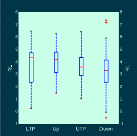
Figure 11: Parallel box plots of real long-term-interest-rate
For the long-term-interest-rate RL no rule can be constructed.
Since it may well be that more than one rule is applicable to one observation, a higher order rule is necessary for the decision which rule should be used. We use the following decision process:
-4 -2 0 2 4 6 8 10 12
Rate of Y
LTP Up UTP
-4 -2 0 2 4 6 8 10 12
Rate of Y
Down
-2 0 2 4 6 8 10 12 14
Rate of LC
LTP Up UTP
-2 0 2 4 6 8 10 12 14
Rate of LC
Down
-1 0 1 2 3 4 5 6 7 8
RL
LTP Up UTP
-1 0 1 2 3 4 5 6 7 8
RL
Down
For each observation of stylized facts, determine the valid rules.
• If there is no valid rule, then randomly decide on the phase corresponding to the frequency of the phases in the learning sample.
• If there is exactly one valid rule, then use this rule.
• If there is more than one valid rule, then use the rule with minimum error, i.e. with the maximum of the maxima of frequencies P of validity of phases.
Example: Consider the following observation:
IE = 0.34, C = 6.13, Y = 5.73, PC = 3.29, PY = 3.98, IC = 2.08, LC = 6.20, L = 2.70 , M1 =11.00, RL = 3.09, RS = 4.83, GD = 3.06, X = 4.57.
Thus, C ≥ 5.56, LC ≥ 5.71, and L ≥ 2.19.
Therefore, the following three rules are applicable with relative frequencies P:
Up UTP Down LTP If C ≥ 5.56 then Down : P = 0.10256 0.30769 0.43590 0.15385 If LC ≥ 5.71 then Down : P = 0.04878 0.12195 0.58537 0.24390 If L ≥ 2.19 then UTP : P = 0.17647 0.52941 0.29412 0
This leads to the application of the 2nd rule, i.e. to the choice of the phase Down.
5. Ranges corresponding to phases
Altogether the above instructions lead to 18 rules, whereof only the following 11 are chosen using the above higher order rule:
phase rule chosen correct
LTP L ≤ -1.32 20 14
IE ≤ -2.73 1 1
Up PY ≤ 2.67 36 28
RS ≤ 4.5 26 13
LC ≤ 2.03 12 8
UTP L ≥ 2.19 8 4
C ≥ 5.56 4 2
IC ≥ 4.98 1 1
Down LC ≥ 5.71 29 18
RS ≥ 7.37 14 7
M1 ≤ 7 4 1
Note that three rules lead to a correct decision in only one case, including the rules based on the growth rate of real-investment-in-construction IC, and the growth rate of money-supply-M1, the variables identified to be ques- tionable stylized facts in chapter 2.
The stylized facts involved in these rules are C, IC, IE, L, LC, M1, PY, and RS. Note that the real-gross- national-product growth rate Y is not used in the rules. The coverage of the rules, when learnt and applied on the whole data set, is 100%, the correctness 63%. Note, however, that the mean prediction error rate found by our standard method leave-one-cycle-out-cross-validation is as high as 54%, which is actually better than the corre- sponding rate for the standard Quadratic Discriminant Analysis (58%), but clearly worse than the corresponding rate for the standard Linear Discrimination Analysis (47%) (Weihs and Garczarek, 2002).
6. Conclusion
Using ad-hoc instructions for identifying univariate rules characterizing the German business cycle 1955-1994, leads to an error rate comparable to standard multivariate methods. Nevertheless, all these error rates are that high that further analysis is urgently necessary (cp. Weihs and Garczarek, 2002).
Literature
Heilemann, U., and Münch, H.-J. (1996): West German Business Cycles 1963-1994: A Multivariate Discriminant Analysis. In: CIRET-Conference in Singapore, CIRET-Studien 50
Lucas, R.E. (1987): Models of Business Cycles. Basil Blackwell
Weihs, C., and Garczarek, U. (2002): Stability of multivariate representation of business cycles over time;
Technical Report 20/2002, SFB 475
Acknowledgement
This work has been supported by the Deutsche Forschungsgemeinschaft (DFG), SFB 475.
We also thank Prof. Dr. U. Heilemann and H.-J. Münch from the RWI (Rheinisch-Westfälisches Institut für Konjunkturforschung) for valuable discussions in our joint project in the SFB 475.