S F B
XXX
E C O N O M I C
R I S K
B E R L I N
SFB 649 Discussion Paper 2015-021
Characterizing the Financial Cycle: Evidence from a Frequency Domain Analysis
Till Strohsal*
Christian R. Proaño**
Jürgen Wolters*
*Freie Universität Berlin, Germany
**The New School of Social Research, United States of America
This research was supported by the Deutsche
Forschungsgemeinschaft through the SFB 649 "Economic Risk".
http://sfb649.wiwi.hu-berlin.de ISSN 1860-5664
SFB 649, Humboldt-Universität zu Berlin
SFB
6 4 9
E C O N O M I C
R I S K
B E R L I N
Characterizing the Financial Cycle:
Evidence from a Frequency Domain Analysis
Till Strohsal
∗a, Christian R. Proaño
b, and Jürgen Wolters
aa
Freie Universität Berlin, Germany
b
The New School of Social Research, New York
April 8, 2015
Abstract
A growing body of literature argues that the financial cycle is considerably longer in duration and larger in amplitude than the business cycle and that its distinguishing features became more pronounced over time. This paper proposes an empirical approach suitable to test these hypothe- ses. We parametrically estimate the whole spectrum of financial and real variables to obtain a complete picture of their cyclical properties. We provide strong statistical evidence for the US and slightly weaker evidence for the UK validating the hypothesized features of the financial cycle. In Germany, however, the financial cycle is, if at all, much less visible.
Keywords: Financial Cycle, Business Cycle, Indirect Spectrum Estimation, Bootstrapping In- ference.
JEL classification: C22, E32, E44.
∗We are grateful for comments and suggestions received from Helmut Lütkepohl, Dieter Nautz, Christian Offermanns, Sven Schreiber, Lars Winkelmann as well as participants of the FU Berlin Macroeconomic Workshop. Financial support from the Deutsche Forschungsgemeinschaft (DFG) through CRC 649 "Economic Risk" is gratefully acknowledged.
E-mail: till.strohsal@fu-berlin.de, proanoac@newschool.edu, juergen.wolters@fu-berlin.de; Phone: +49 (0)30 838-53399.
1 Introduction
Fluctuations in financial markets play a key role in the macroeconomic dynamics of modern economies, often leading to either significant economic booms or severe economic crises, see e.g. Kindleberger and Aliber(2005) andSchularick and Taylor(2012). The last twenty years provide several examples, from Japan’s lost decade following the asset market crash in the early 1990s to the 2007-08 global financial crisis which led the world economy to the brink of a new Great Depression. Against this background, a renewed interest in financial market dynamics is emerging. A growing body of literature argues that the cyclical behavior of financial aggregates may be understood not only as a pure reflection of the real side of the economy, but also as the result of underlying changes in the general perception and attitudes towards financial and macroeconomic risk, seeCaballero (2010) for a survey.
The distinguishing feature of the financial cycle, as put forward in recent studies, is that its duration and amplitude are considerably longer and larger than those of the classical business cycle, see e.g.
Claessens et al.(2011). Borio(2014), for instance, suggests that the financial cycle operates at lower, medium-term frequencies, with a cycle length between eight and thirty years. This extended length of the financial cycle is often considered to reflect the build-up of macro-financial instability, most recently contributing to the 2007-08 financial crisis. Despite its crucial importance for macroeconomic developments, however, it is not clear how the financial cycle should be empirically analyzed.
Most of the existing insights into the characteristics of the financial cycle are based on either the analysis of turning points (Claessens et al.,2011,2012) or frequency-based filter methods (Drehmann et al.,2012). The turning point approach requires a pre-specified rule which is applied to an observed time series in order to find local maxima and minima. Frequency-based filter methods require a pre-specified frequency range at which the financial cycle is assumed to operate. Therefore, both approaches are quite descriptive and do not allow to test the hypothesized characteristics of the financial cycle. Indeed, while there is a broad consensus in the literature concerning the fundamental characteristics of the business cycle (see e.g. Diebold and Rudebusch,1996 for a survey), this is not yet true for the financial cycle.
This paper proposes a straightforward econometric methodology to obtain a complete picture of the cyclical properties of key financial aggregates. Making use of the fact that any covariance-stationary stochastic process can be equivalently represented in the time and in the frequency domain, we apply a parametric method to estimate spectral densities. That is, we fit time series models from the autoregressive moving average (ARMA) class to standard financial activity indicators and use the estimated processes to compute their corresponding frequency domain representations. This enables us to get an overview of the length and relevance, in terms of variance contributions, of cycles at all possible frequencies. Hence, our approach eliminates the need toa priori assume a range where the financial cycle operates. Moreover, it is an inferential method in the sense that it allows us to test existing hypotheses by statistical means.
Specifically, we use the estimated spectral densities and their bootstrap standard errors to address the following questions. First, has the financial cycle a longer duration, as well as a larger amplitude than the classical business cycle? Second, have the characteristics of the financial cycle changed over time?
Our main results are as follows. Strong evidence is found in support of the hypothesized features of the financial cycle in the United States. Somewhat weaker evidence is provided for the United Kingdom. In the case of Germany, distinct characteristics of the financial cycle are, if at all, much less visible.
The remainder of this paper is organized as follows. Section2motivates and discusses our methodology in detail. Section 3 contains our empirical results on the financial cycle in the US, the UK, and Germany. Finally, we draw some concluding remarks in Section 4.
2 Methodology
2.1 Existing Approaches: Analysis of Turning Points and Frequency-Based Filters
The first important empirical approach to assess the financial cycle is the traditional turning point analysis. The method goes back to Bry and Boschan (1971) and is adapted to quarterly data by Harding and Pagan(2002). While originally used to analyze business cycles, recent studies ofClaessens et al.(2011,2012) andDrehmann et al.(2012) adopted it to investigate financial cycles. The turning point analysis requires a pre-specified rule which defines a complete cycle in terms of the minimum number of periods of increases (expansion phase) and decreases (recession phase). Therefore, this method is descriptive in nature and hypotheses testing is not possible.
The second prominent approach is to work with frequency-based filters (Drehmann et al.,2012) which are usually based onBaxter and King(1999) or refinements thereof, see e.g. Christiano and Fitzgerald (2003). When filters are used to analyze cycles, a crucial point is that the frequency range has to be pre-specified by the researcher. This may lead to results biased into the direction of the pre- defined range. The intuition behind this difficulty is best described by briefly discussing the general functioning of filters.
In the time domain, any linear filter can be written in the form of a two-sided moving average yt=
Xn
j=−m
ajxt−j . (1)
The filtered series yt depends simultaneously on the properties of the filter (the coefficients aj) and the data (the observed series xt). To convert equation (1) into the frequency domain, one uses the corresponding filter function
C(λ) = Xn
j=−m
aje−iλj , i2=−1, (2)
and its transfer function
T(λ) =|C(λ)|2 , (3)
where λ∈ [−π, π] denotes the frequency range, see e.g. Wolters (1980a, 1980b). The relationship between the spectra of the original and the filtered series is given by
fy(λ) =T(λ)fx(λ). (4)
When compared to the time domain, a major advantage of the representation in (4) is that now the filter effect T(λ) is separated from the data fx(λ). For the spectrum of the filtered series fy(λ) to accurately identify cycles in the spectrum of the observed seriesfx(λ), the ideal filter candidate would be the one that has the value 1 at the frequency range of interest [λlow, λhigh] and 0 otherwise. In view of equation (4), this is because T(λ) = 1 implies fy(λ) =fx(λ) for λ ∈[λlow, λhigh] and fy(λ) = 0 for λ /∈[λlow, λhigh]. Theoretically, the ideal time domain filter can be achieved by moving averages of infinite order. Yet, in practice, this is not possible since only a limited number of observations is available.
The main idea of frequency-based filters is to pre-specify a range from λlowto λhigh, to choose finite values for m and nin equation (1) and to find the weights aj which approximate the ideal filter as good as possible. Due to the approximation, the spectrum of the filtered series is in general different from the one of the observed series in [λlow, λhigh] and reflects a mixture of filter and data properties in the form ofT(λ)fx(λ). More precisely, it can be shown that any filter has the tendency to overstate the contributions of cycles in the pre-defined frequency range [λlow, λhigh] to the overall variance of the underlying time series. Because of this tendency, artificial cycles may be produced even if the true data generating process has no cycles.1
In this study, we emphasize that the appropriate λlow and λhigh are unknown. Indeed, while there seems to be general consensus in the literature about the relevant frequency range for the business cycle (2 to 8 years), the relevant frequency range for the financial cycle is less clear. For instance, Drehmann et al.(2012) construct their financial cycle measure from the underlying series witha priori chosen cycle length between 8 and 30 years.
2.2 An Alternative Approach: Parametric Estimation of Spectral Densities
This paper proposes a simple method to characterize cycles in the frequency domain. Instead of focusing on certain frequency ranges, we analyze the complete spectrum. Our approach seeks to use statistical methods to exploit all the information included in the data.
It is known that any covariance-stationary process has a time domain and a frequency domain repre- sentation which are fully equivalent.2 However, when compared with the time domain representation,
1This issue has been raised already in the 1950’s and 1960’s. For a discussion of the general problem see e.g. König and Wolters(1972),Baxter and King(1999),Christiano and Fitzgerald(2003) andMurray(2003).
2This was first discussed inWiener(1930) andKhintchine(1934).
the frequency domain representation is more suited to the analysis of cyclical features, as the impor- tance of certain cycles for the total variation of the process can be easily derived from the spectrum.3 This is possible because the spectrum represents an orthogonal decomposition of the variance of the process.
The starting point of the indirect spectrum estimation is to specify the DGP of the underlying time series as an ARMA model:
A(L)xt=δ+B(L)ut , ut∼WN(0, σ2) . (5) In equation (5),A(L) andB(L) denote polynomials in the lag operatorLof orderpandq, respectively.
For stable processes, the MA(∞) representation has the form xt−µ=B(L)
A(L)ut , µ= δ
A(1) . (6)
Equation (6) shows that an ARMA representation can be interpreted as an estimated filter that transforms the white noise processutinto the observed time seriesxt. This filter is of infinite length but depends only on a finite number of parameters. The ARMA model is in fact a filter which captures the whole dynamics of the observed process xt in form of its complete spectrum from−π to π. In direct analogy to equation (4) it holds that
fx(λ) = |B(e−iλ)|2
|A(e−iλ)|2fu(λ) , (7)
where |B(e−iλ)|2/|A(e−iλ)|2 = T(λ) and fu(λ) = σ2π2 as the spectrum of the white noise process.
Equation (7) represents theindirect spectrum estimationand allows us to derive the cyclical properties ofxt.4
Fromfx(λ) we can identify, without anya priori assumptions, which frequency range is most relevant for the dynamics of the time series under consideration in terms of its variance contribution. The spectrum will exhibit a peak at a given frequency if cyclical variations occurring around that frequency are particularly important for the overall variation of the process. Also, if spectral mass is more concentrated in a given range around the peak, the corresponding cycle will show a larger amplitude causing more regular process fluctuations in the time domain. Normalizing the spectrum by the process variance5, one obtains the spectral density which provides the relative contributions of particular frequencies to the total variance of the process.
To statistically assess the characteristics of the financial cycle across variables and different sample periods, the inference in the empirical part will be based on bootstrap methods.6 We apply the following bootstrap procedure, see e.g. Benkwitz et al.(2001).
3Technically, the spectrum is the Fourier transformation of the autocovariance function.
4This is a valid approach, as “If the model is correctly specified, the maximum likelihood estimates [of the ARMA(p,q) model] will get closer and closer to the true values as the sample size grows; hence, the resulting estimate of the population spectrum should have this same property” (Hamilton,1994, p.167).
5The process variance is calculated by numerically integrating the spectrum.
6To the best of our knowledge, analytical expressions for such standard errors are not available.
1. Estimate the parameters of the ARMA model in equation (5).
2. Generate bootstrap residualsu∗1, . . . , u∗T by randomly drawing with replacement from the set of estimated residuals.
3. Construct a bootstrap time series recursively using the estimated parameters from step 1 and the bootstrap residuals from step 2.
4. Reestimate the parameters from the data generated in step 3.
5. Repeat step 2 to step 4 5000 times.
6. From the bootstrap distributions of the statistics of interest, e.g., cycle length, amplitude etc., we compute the standard errors and the corresponding 95% confidence intervals.
An obvious alternative to the indirect parametric estimation would be the direct non-parametric estimation of the spectrum, see e.g. Fishman (1969).7 In order to get consistent estimates, however, one has to use a kernel estimator. Such estimates depend heavily on the chosen kernel and its bandwidth parameterM, implying that a large amount of observation is required to have the necessary degrees of freedom. For instance, if we estimate the spectrum fromTobservations by transforming the firstM estimated autocovariances, we haveC·MT degrees of freedom. The constantCis kernel-specific and usually takes on values of around 3. A small value of M decreases the variance but increases the bias of the estimator. Having in mind the data in our empirical analysis below, let us consider a sample size ofT = 100. In that case, a reasonable choice for M maybe 20, leading to only about 15 degrees of freedom. In contrast, the indirect estimation approach, starting from an ARMA model with e.g. 5 parameters, leaves us with 95 degrees of freedom and hence implies a strong efficiency gain.
3 Empirical Analysis
3.1 Data Description: Indicators of Financial and Real Developments
As perceptions and risk attitudes are not directly observable it is unclear which particular financial indicator or set of financial variables might reflect the financial cycle best.8 In the following analysis we use the most common proxy variables for the financial cycle; quarterly, seasonally adjusted aggregate
7For an empirical analysis of US business cycles via directly estimated spectra seeSargent(1987).
8On the one hand, in Drehmann et al.(2012) andBorio(2014) it is argued that the financial cycle can be most parsimoniously described in terms of credit and property prices. On the other hand, other studies such asEnglish et al.
(2005),Ng(2011), andHatzius et al.(2010) have used principal components and factor analysis to identify the common factors of a number of financial price and quantity variables for the characterization of the financial cycle. Recently, Breitung and Eickmeier(2014) use a multi-level dynamic factor model to extract the main driving forces behind business and financial cycles at an international level using a large set of macroeconomic and financial indicators.
data on credit volume, the credit to GDP ratio, house prices and equity prices, see Claessens et al.
(2011, 2012) andDrehmann et al.(2012). Real GDP is taken as a proxy for the business cycle. We study three representative industrialized countries: the US, the UK, and Germany.9
To allow for a meaningful comparison to existing studies, we employ data transformations similar to those found in Drehmann et al.(2012). All series are measured in logs, deflated with the consumer price index and normalized by their respective value in 1985Q1 to ensure comparability of units.
Growth rates are obtained by taking annual differences of each time series.10 The only exception is the credit to GDP ratio which is expressed in percentage points and measured in deviations from a linear trend.11 We use the longest possible sample for each individual time series which is mostly 1960Q1 until 2013Q4 for the US and the UK, see Figures7and8. Due to data availability the German time series start only in 1970Q1, see Figure9.
We split the data in two subsamples to analyze possible changes in the characteristics of the financial cycles over time. According to Claessens et al. (2011, 2012) andDrehmann et al.(2012), the break point is specified at 1985Q1 for the US and UK.12 In the case of Germany, we choose the break point close to the German reunification, 1990Q2.13
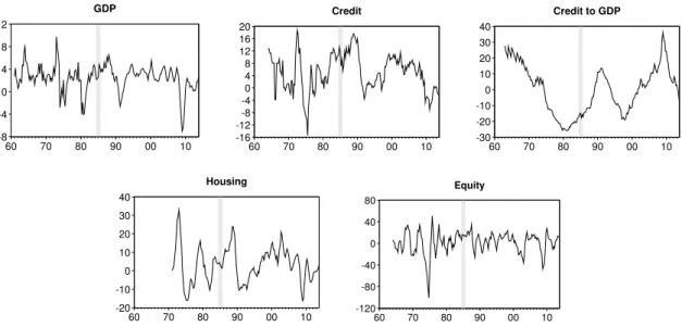
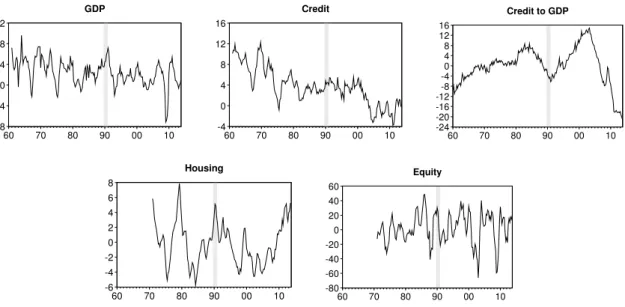
All data used in the analysis are shown in Figures1 to 3, where the vertical gray line highlights the sample split. A first visual inspection of the real GDP dynamics suggests that the amplitude of the US GDP growth rate fluctuations diminished from the 1990’s until the outbreak of the 2007-08 global financial crisis, when real GDP dropped by about 4%. This seems to be different, however, in the UK and Germany, where the variance of the GDP growth rate appears to have remained more or less constant. Compared to GDP, the credit and house price growth rates show more pronounced swings in the US and the UK. In Germany, this is only true for housing. The last graphs in Figures1 to 3 illustrate the dynamics of equity prices in the three countries. As it can be observed, these series not only feature a high volatility, but their dynamics seem to be very different from the previous proxy variables for the financial cycle.
9A more detailed description of the definition and sources of the variables can be found in AppendixA.
10This implies that we investigate cycles in growth rates.
11Unit root tests of the level series indicate that, with the exception of the credit to GDP ratios which are found to be trend-stationary, all other time series can be considered as integrated of order one. Therefore, working with annual growth rates for GDP, credit, housing and equity, i.e., annually differencing the data, is in line with the unit root test results. In the case of the credit to GDP ratio, we eliminated a deterministic linear trend. Results are available upon request.
12This is often seen as the starting point of the financial liberalization phase in mature economies. Moreover, during this period monetary policy regimes being more successful in controlling inflation are established, seeBorio(2014).
13From 1990Q2 on, official data for the unified Germany are available.
-6 -4 -2 0 2 4 6 8 10
60 70 80 90 00 10
GDP
-6 -4 -2 0 2 4 6 8 10 12
60 70 80 90 00 10
Credit
-20 -10 0 10 20 30
60 70 80 90 00 10
Credit to GDP
-16 -12 -8 -4 0 4 8
60 70 80 90 00 10
Housing
-50 -40 -30 -20 -10 0 10 20 30 40
60 70 80 90 00 10
Equity
Figure 1: Real GDP and Financial Cycle Proxy Variables in the United States. Note: All series are annual growth rates, except the credit to GDP ratio, which represents deviations from a linear trend measured in percentage points. The vertical gray line shows the sample split.
-8 -4 0 4 8 12
60 70 80 90 00 10
GDP
-16 -12 -8 -4 0 4 8 12 16 20
60 70 80 90 00 10
Credit
-30 -20 -10 0 10 20 30 40
60 70 80 90 00 10
Credit to GDP
-20 -10 0 10 20 30 40
60 70 80 90 00 10
Housing
-120 -80 -40 0 40 80
60 70 80 90 00 10
Equity
Figure 2: Real GDP and Financial Cycle Proxy Variables in the United Kingdom. Note: All series are annual growth rates, except the credit to GDP ratio, which represents deviations from a linear trend measured in percentage points. The vertical gray line shows the sample split.
-8 -4 0 4 8 12
60 70 80 90 00 10
GDP
-4 0 4 8 12 16
60 70 80 90 00 10
Credit
-24 -20 -16 -12 -8 -4 0 4 8 12 16
60 70 80 90 00 10
Credit to GDP
-6 -4 -2 0 2 4 6 8
60 70 80 90 00 10
Housing
-80 -60 -40 -20 0 20 40 60
60 70 80 90 00 10
Equity
Figure 3: Real GDP and Financial Cycle Proxy Variables in Germany. Note: All series are annual growth rates, except the credit to GDP ratio, which represents deviations from a linear trend measured in percentage points. The vertical gray line shows the sample split.
3.2 Time Domain Estimation Results and Frequency Domain Representation
The empirical estimates of the spectral densities are based on the ARMA models reported in Tables 7 to 9 in AppendixB.14 The model specification procedure follows the principle of parsimony. We initially allow for a maximum autoregressive order of 5 and subsequently remove any remaining residual autocorrelation by the inclusion of appropriate moving average terms. As reported in Tables7 to 9, all parameters in the final specifications are statistically significant at standard confidence levels and the estimated residuals are free from autocorrelation according to the Lagrange multiplier (LM) test.
In order to provide an example of how we use the estimated ARMA models to obtain the spectral densities, consider the following process of US real GDP growth during the pre-1985 period with t-values in parentheses (cf. Table7) and the notation as in equation (5):
xt= 0.002
(2.97)+ 1.144
(19.21)xt−1−0.224
(−4.37)xt−3−0.985
(−42.04)ut−4+ut .
These estimates are applied to equation (7) to calculate the corresponding spectrum as fx(λ) = |1−0.985e−i4λ|2
|1−1.144e−iλ+ 0.224e−i3λ|2 σ2 2π ,
14To statistically double-check the specified break dates, we also estimated ARMA models for the full sample. Chow breakpoint tests show overwhelming evidence for a break at 1985Q1 for the US and the UK. For Germany, the statistical support for a break at 1990Q2 is weaker, but for GDP and credit we clearly reject the null hypothesis of no break.
Nonetheless, the German reunification is a natural break date from an economic point of view.
with e−iλ = cos(λ)−i·sin(λ) by Euler’s relation and i2 = −1. According to this procedure, we calculated the spectra for all countries and sample periods under consideration. Dividing fx(λ) by the variance of xtyields the spectral densities.
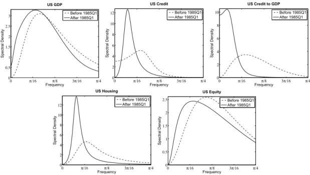
The estimated spectral densities are shown in Figures4to 6in the range [0, π/4], i.e., for periods of
∞to 2 year.15 We do not show frequencies in [π/4, π] since almost no spectral mass is located in this range. The frequency π/16 corresponds to 8 years and separates the financial cycle range from the business cycle range. An initial visual inspection of Figures 4 to 6 delivers at least two noteworthy results.
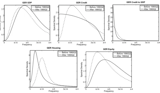
First, especially for the US and UK the spectral densities of credit, credit to GDP and house prices are substantially shifted to the left in the later period compared to the first one, indicating - at least superficially - that longer cycles became present, see Figures 4 and 5. Moreover, the peaks of the spectral densities are much more pronounced, suggesting that these longer cycles are also more important for the variation of the process. For Germany, as illustrated in Figure 6, this is only true for house prices. We obtain no clear results for German credit and credit to GDP. Therefore, German data does not provide much evidence in favor of the postulated financial cycle properties.
Second, Figures4,5 and6clearly show that in all three countries, the spectral densities of GDP and equity changed very little from the period before the sample split to the one thereafter. The interesting exception is the spectrum of UK GDP growth which may indeed have experienced a change. The general impression, however, is that in almost all cases GDP and equity show very similar spectral shapes with less pronounced peaks compared to the other variables. Thus, it seems that if financial markets actually reflect the real side of the economy, then this is only visible in equity prices.
Having obtained a frequency representation of the time series under consideration which is particularly suitable for the analysis of their cyclical properties, we continue in the next section by statistically testing various hypotheses concerning key features of the financial cycle which have been postulated in recent studies.
15When using quarterly data, all cycles of length infinity to half a year are described by the spectrum in the range from 0 toπbecausefx(λ) is an even symmetric continuous function. We approximate the continuous spectrum by 1000 equally spaced frequency bands from 0 toπ.
0 π/16 π/8 3π/16 π/4 0
0.5 1 1.5 2 2.5 3
Frequency
Spectral Density
US GDP
Before 1985Q1 After 1985Q1
0 π/16 π/8 3π/16 π/4
0 2 4 6 8 10 12
Frequency
Spectral Density
US Credit
Before 1985Q1 After 1985Q1
0 π/16 π/8 3π/16 π/4
0 2 4 6 8 10
Frequency
Spectral Density
US Credit to GDP
Before 1985Q1 After 1985Q1
0 π/16 π/8 3π/16 π/4
0 2 4 6 8 10 12
Frequency
Spectral Density
US Housing
Before 1985Q1 After 1985Q1
0 π/16 π/8 3π/16 π/4
0 0.5 1 1.5 2 2.5
Frequency
Spectral Density
US Equity
Before 1985Q1 After 1985Q1
Figure 4: Spectral Densities in the US. Note: Figures show the spectral densities from frequency zero to π/4, corresponding to a cycle length of infinity to 2 year. Frequencyπ/16 corresponds to 8 years.
0 π/16 π/8 3π/16 π/4
0 1 2 3 4
Frequency
Spectral Density
UK GDP
Before 1985Q1 After 1985Q1
0 π/16 π/8 3π/16 π/4
0 2 4 6 8
Frequency
Spectral Density
UK Credit
Before 1985Q1 After 1985Q1
0 π/16 π/8 3π/16 π/4
0 2 4 6 8
Frequency
Spectral Density
UK Credit to GDP
Before 1985Q1 After 1985Q1
0 π/16 π/8 3π/16 π/4
0 2 4 6 8 10
Frequency
Spectral Density
UK Housing
Before 1985Q1 After 1985Q1
0 π/16 π/8 3π/16 π/4
0 0.5 1 1.5 2 2.5
Frequency
Spectral Density
UK Equity
Before 1985Q1 After 1985Q1
Figure 5: Spectral Densities in the UK. Note: Figures show the spectral densities from frequency zero to π/4, corresponding to a cycle length of infinity to 2 year. Frequencyπ/16 corresponds to 8 years.
0 π/16 π/8 3π/16 π/4 0
0.5 1 1.5 2 2.5
Frequency
Spectral Density
GER GDP
Before 1990Q2 After 1990Q2
0 π/16 π/8 3π/16 π/4
0 0.5 1 1.5 2 2.5 3
Frequency
Spectral Density
GER Credit
Before 1990Q2 After 1990Q2
0 π/16 π/8 3π/16 π/4
0 5 10 15 20 25 30 35
Frequency
Spectral Density
GER Credit to GDP Before 1990Q2 After 1990Q2
0 π/16 π/8 3π/16 π/4
0 2 4 6 8
Frequency
Spectral Density
GER Housing
Before 1990Q2 After 1990Q2
0 π/16 π/8 3π/16 π/4
0 0.5 1 1.5 2 2.5 3
Frequency
Spectral Density
GER Equity
Before 1990Q2 After 1990Q2
Figure 6: Spectral Densities in Germany. Note: Figures show the spectral densities from frequency zero toπ/4, corresponding to a cycle length of infinity to 2 year. Frequencyπ/16 corresponds to 8 years.
3.3 Characterizing Business and Financial Cycles from a Frequency Domain Perspective
Statistics to Characterize Cycles
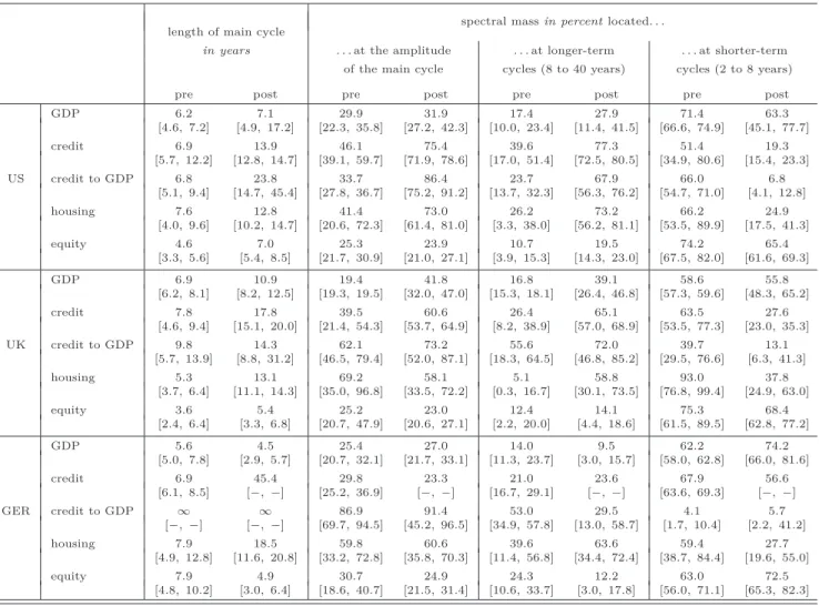
We propose 4 different statistics derived from the spectral densities to describe the main features of business and financial cycles. Table1 summarizes the statistics for all countries under consideration and the two estimation subsamples. The first two columns of Table1 include the main cycle length in years measured at the peak of the spectrum. It is given by λ2πmax withλmax as the frequency where the spectral density has its unique maximum. The remaining columns include information about the distribution of the spectral mass measured in percentage points. For instance, we report the spectral mass located around the amplitude of the main cycle. The amplitude is defined as the spectral mass in the frequency band symmetric around λmax with a length of about 20π.16 The last four columns present estimates of the spectral mass for pre-defined ranges which are often used in the literature, i.e., 8 to 40 years for the financial cycle and 2 to 8 years for the business cycle. The values in brackets below the point estimates are the 95% bootstrap confidence intervals.
16This frequency band is defined asλmax± π
1000·25.
Table 1: Frequency Domain: Length and Variance Contribution of Cycles
spectral massin percentlocated. . . length of main cycle
in years . . . at the amplitude . . . at longer-term . . . at shorter-term of the main cycle cycles (8 to 40 years) cycles (2 to 8 years)
pre post pre post pre post pre post
GDP 6.2 7.1 29.9 31.9 17.4 27.9 71.4 63.3
[4.6,7.2] [4.9,17.2] [22.3,35.8] [27.2,42.3] [10.0,23.4] [11.4,41.5] [66.6,74.9] [45.1,77.7]
credit 6.9 13.9 46.1 75.4 39.6 77.3 51.4 19.3
[5.7,12.2] [12.8,14.7] [39.1,59.7] [71.9,78.6] [17.0,51.4] [72.5,80.5] [34.9,80.6] [15.4,23.3]
US credit to GDP 6.8 23.8 33.7 86.4 23.7 67.9 66.0 6.8
[5.1,9.4] [14.7,45.4] [27.8,36.7] [75.2,91.2] [13.7,32.3] [56.3,76.2] [54.7,71.0] [4.1,12.8]
housing 7.6 12.8 41.4 73.0 26.2 73.2 66.2 24.9
[4.0,9.6] [10.2,14.7] [20.6,72.3] [61.4,81.0] [3.3,38.0] [56.2,81.1] [53.5,89.9] [17.5,41.3]
equity 4.6 7.0 25.3 23.9 10.7 19.5 74.2 65.4
[3.3,5.6] [5.4,8.5] [21.7,30.9] [21.0,27.1] [3.9,15.3] [14.3,23.0] [67.5,82.0] [61.6,69.3]
GDP 6.9 10.9 19.4 41.8 16.8 39.1 58.6 55.8
[6.2,8.1] [8.2,12.5] [19.3,19.5] [32.0,47.0] [15.3,18.1] [26.4,46.8] [57.3,59.6] [48.3,65.2]
credit 7.8 17.8 39.5 60.6 26.4 65.1 63.5 27.6
[4.6,9.4] [15.1,20.0] [21.4,54.3] [53.7,64.9] [8.2,38.9] [57.0,68.9] [53.5,77.3] [23.0,35.3]
UK credit to GDP 9.8 14.3 62.1 73.2 55.6 72.0 39.7 13.1
[5.7,13.9] [8.8,31.2] [46.5,79.4] [52.0,87.1] [18.3,64.5] [46.8,85.2] [29.5,76.6] [6.3,41.3]
housing 5.3 13.1 69.2 58.1 5.1 58.8 93.0 37.8
[3.7,6.4] [11.1,14.3] [35.0,96.8] [33.5,72.2] [0.3,16.7] [30.1,73.5] [76.8,99.4] [24.9,63.0]
equity 3.6 5.4 25.2 23.0 12.4 14.1 75.3 68.4
[2.4,6.4] [3.3,6.8] [20.7,47.9] [20.6,27.1] [2.2,20.0] [4.4,18.6] [61.5,89.5] [62.8,77.2]
GDP 5.6 4.5 25.4 27.0 14.0 9.5 62.2 74.2
[5.0,7.8] [2.9,5.7] [20.7,32.1] [21.7,33.1] [11.3,23.7] [3.0,15.7] [58.0,62.8] [66.0,81.6]
credit 6.9 45.4 29.8 23.3 21.0 23.6 67.9 56.6
[6.1,8.5] [−,−] [25.2,36.9] [−,−] [16.7,29.1] [−,−] [63.6,69.3] [−,−]
GER credit to GDP ∞ ∞ 86.9 91.4 53.0 29.5 4.1 5.7
[−,−] [−,−] [69.7,94.5] [45.2,96.5] [34.9,57.8] [13.0,58.7] [1.7,10.4] [2.2,41.2]
housing 7.9 18.5 59.8 60.6 39.6 63.6 59.4 27.7
[4.9,12.8] [11.6,20.8] [33.2,72.8] [35.8,70.3] [11.4,56.8] [34.4,72.4] [38.7,84.4] [19.6,55.0]
equity 7.9 4.9 30.7 24.9 24.3 12.2 63.0 72.5
[4.8,10.2] [3.0,6.4] [18.6,40.7] [21.5,31.4] [10.6,33.7] [3.0,17.8] [56.0,71.1] [65.3,82.3]
Notes: The cycle length is defined as λmax2π , whereλmaxis the frequency where the spectral density has its unique maximum. The amplitude of the main cycle is defined as the spectral mass in the frequency band symmetric aroundλmaxwith a length of about20π. The termspre andpostrefer to the sample periods 1960Q1 until 1984Q4 and 1985Q1 until 2013Q4, respectively, for the US and the UK. In the case of
12
As reported in Table1, our indirect estimation approach delivers estimates in line with the literature.
For instance, the average length of the business cycle (as described by GDP growth) is 6.2, 6.9 and 5.6 years in the US, UK, and Germany, respectively, in the first subsample, and 7.1, 10.9 and 4.5 in the second subsample. This confirms – with a single exception – the standard notion that business cycle fluctuations have a duration between 2 and 8 years, see Hodrick and Prescott(1997).
Hypotheses Tests
For our tests of the hypotheses on the properties of the financial cycle, we confine our attention to two series, credit and housing, and refrain from including results for credit to GDP and equity. There are several reasons for this decision. Equity shows no dynamic property related to stated characteristics of financial cycles in any of the countries studied. The results for credit to GDP are very similar to those obtained from credit alone, making use of credit to GDP redundant. Further, following Borio (2014), credit and house prices should capture the most important features of financial cycles. Credit represents a direct financing constraint and house prices are seen as a proxy variable for the average perception of value and risk in the economy.
As a starting point, we test whether the financial cycle tends to be a medium-term phenomenon with a longer cycle length than that of the business cycle as suggested byClaessens et al.(2011),Drehmann et al. (2012) and Borio (2014). This addresses the key question, are financial market fluctuations mere reflections of the business cycle, in which case they should operate at similar frequencies, or are financial market fluctuations driven by intrinsic and self-reinforcing forces which would make such fluctuations last longer, and feature a larger amplitude.
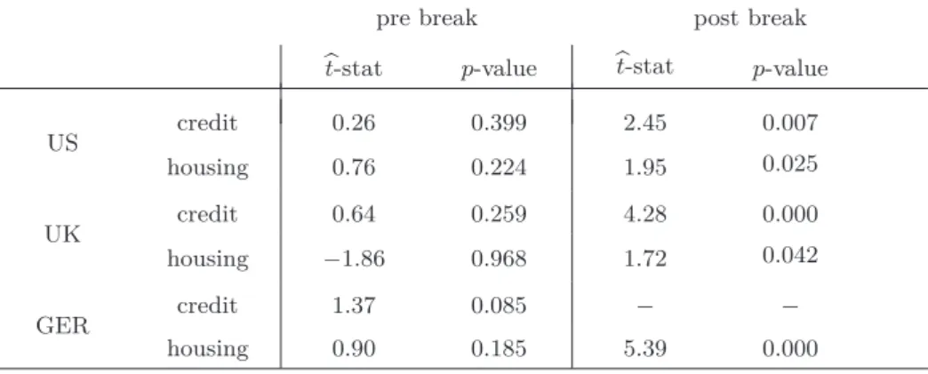
Table2reports the test results of the null hypothesis that the financial cycle and the business cycle are of equal length against the alternative hypothesis that the financial cycle is longer than the business cycle. According to one-sided two-sample t-tests, the null hypothesis cannot be rejected in the first subsample for any of the countries. This is no longer true in the second subsample, where the null is rejected at all conventional confidence levels. With respect to the estimation results in Table 1 this is not surprising. In the second subsample the average business cycle across the three countries is 7.5 years, while the average financial cycle of 15.2 years – excluding German credit – is twice as long.
We then consider if the medium-term nature of the financial cycle is a recent phenomenon, i.e., has the length of the cycle increased over time. Statistical evidence is shown in Table3. The results clearly support the hypothesis that the financial cycle is indeed longer during the second sample period. The mean value of the financial cycle length across the three countries more than doubled, from about 7 years in the first period, to almost 16 years in the second period. These findings, together with the test results reported in Table 2, not only corroborate the insights gleaned from Figures4, 5 and 6 – where a general left-shift of the spectral densities of credit and housing growth (as well as of the credit-to-GDP ratio) can be observed – but they also deliver statistical support for the descriptive findings ofClaessens et al.(2011),Drehmann et al.(2012) andBorio(2014).
Table 2: Is the Financial Cycle Longer Than the Business Cycle?
H0: The financial cycle and the business cycle are of equal length.
H1: The financial cycle is longer than the business cycle.
pre break post break
b
t-stat p-value bt-stat p-value
US credit 0.26 0.399 2.45 0.007
housing 0.76 0.224 1.95 0.025
UK credit 0.64 0.259 4.28 0.000
housing −1.86 0.968 1.72 0.042
GER credit 1.37 0.085 − −
housing 0.90 0.185 5.39 0.000
Notes:bt-stat represents the estimated value of thet-statistic of a one-sided two-samplet-test. By
”−” it is indicated that we could not obtain finite bootstrap standard deviations which implies that it is not possible to conduct at-test.
Table 3: Has the Financial Cycle Increased in Length Over Time?
H0: The length of the financial cycle has not changed over time.
H1: The length of the financial cycle has increased over time.
b
t-stat p-value
US credit 2.32 0.010
housing 2.59 0.005
UK credit 5.69 0.000
housing 7.26 0.000
GER credit − −
housing 3.01 0.001
Notes:bt-stat represents the estimated value of thet-statistic of a one-sided two-samplet-test that compares the cycle lengths in the pre and post sample period. By ”−” it is indicated that we could not obtain finite bootstrap standard deviations which implies that it is not possible to conduct at-test.
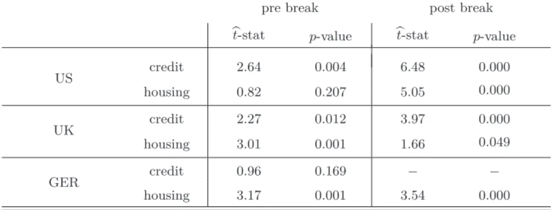
Next, we investigate the variance contributions of given frequency ranges to analyze the relevance of the financial cycle. First, we test whether the financial cycle and the business cycle featured the same amplitude in the two analyzed subperiods. Table4shows somewhat mixed evidence in the first sample period. In most cases we reject the null of equal amplitudes of business and financial cycles.
For US house prices and German credit, however, a rejection is not possible. In the second period, the results are much clearer. The null hypothesis is rejected for all variables in all countries. This indicates that, particularly in recent times, the financial cycle is characterized by a larger amplitude than the business cycle.
Table 4: Has the Financial Cycle a Larger Amplitude Than the Business Cycle?
H0: The financial cycle and the business have the same amplitude.
H1: The financial cycle has a larger amplitude than the business cycle.
pre break post break
bt-stat p-value bt-stat p-value
US credit 2.64 0.004 6.48 0.000
housing 0.82 0.207 5.05 0.000
UK credit 2.27 0.012 3.97 0.000
housing 3.01 0.001 1.66 0.049
GER credit 0.96 0.169 − −
housing 3.17 0.001 3.54 0.000
Notes: The approximate amplitude is defined as the spectral mass in the symmetric frequency band with a length of about 20π aroundλmax, whereλmaxis the frequency where the spectral density has its unique maximum.bt-stat represents the estimated value of thet-statistic of a one-sided two-sample t-test. By ”−” it is indicated that we could not obtain finite bootstrap standard deviations which implies that it is not possible to conduct at-test.
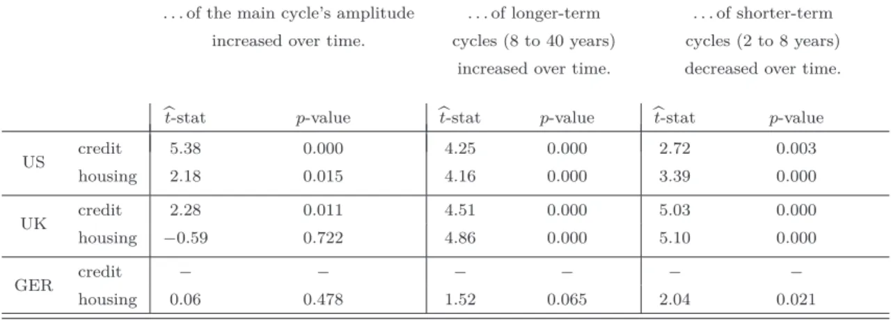
Finally, we investigate whether the financial cycle has become more important over time in terms of its variance contribution. We address this question by testing whether the main cycle’s amplitude has increased, whether the contribution of longer-term cycles to the overall variation of the process has increased, and whether the variance contribution of shorter-term (business) cycles has decreased.
As can be seen from Table 5, thet-tests strongly support the alternative hypothesis of a significant increase for the US using both the credit and housing series. In the UK, the t-test results deliver a significant result only for the credit series. Germany seems again to be characterized by different dynamics, as the main cycle’s amplitude of the house price series does not appear to have changed between the two time periods.
We also find strong statistical evidence supporting the idea that the contribution of longer-term cycles
Table 5: Has the Importance of the Financial Cycle Increased Over Time?
H0: The relevance of longer-term cycles has not changed over time.
That is, the variance contribution. . .
. . . of the main cycle’s amplitude . . . of longer-term cycles . . . of shorter-term cycles remained constant over time. (8 to 40 years) remained (2 to 8 years) remained
constant over time. constant over time.
H1: Longer-term cycles became more important in recent decades.
That is, the variance contribution. . .
. . . of the main cycle’s amplitude . . . of longer-term . . . of shorter-term increased over time. cycles (8 to 40 years) cycles (2 to 8 years)
increased over time. decreased over time.
bt-stat p-value bt-stat p-value bt-stat p-value
US credit 5.38 0.000 4.25 0.000 2.72 0.003
housing 2.18 0.015 4.16 0.000 3.39 0.000
UK credit 2.28 0.011 4.51 0.000 5.03 0.000
housing −0.59 0.722 4.86 0.000 5.10 0.000
GER credit − − − − − −
housing 0.06 0.478 1.52 0.065 2.04 0.021
Notes: The approximate amplitude is defined as the spectral mass in the symmetric frequency band with a length of about 20π aroundλmax, whereλmaxis the frequency where the spectral density has its unique maximum. bt-stat
represents the estimated value of thet-statistic of a one-sided two-samplet-test. By ”−” it is indicated that we could not obtain finite bootstrap standard deviations which implies that it is not possible to conduct at-test.
in the dynamics of credit and housing has increased over time, both for the US and the UK, but much less significantly for Germany. This is further supported by the test results in the last two columns in Table5which suggest that the variance contribution of shorter-term cycles in credit and housing has significantly decreased in the US and UK, and, to a lesser extent, in Germany. Put differently, these results indicate a significant change of the overall shape of the spectral density over time. In more recent times, the largest share of spectral mass of the credit and housing series in the US and UK is clearly located at cycles longer than the business cycle. This conclusion does not seem to bear out for the house price dynamics in Germany, however, medium-term frequencies do seem to have become somewhat more relevant in the second period.
4 Concluding Remarks
What are the main characteristics of the financial cycle?17 Is it a medium-term phenomenon, meaning it is longer than the business cycle, as suggested in the literature, or does it share similar characteristics with the business cycle? Has its importance increased over time? Or is it tied to the business cycle in a way that makes analysis of the financial cycle a redundant exercise? In this paper we intended to shed some light on these and other related questions. We did that by estimating the data generating processes of financial and business cycle variables using econometric methods, in contrast to the more descriptive approaches pursued by Claessens et al. (2011, 2012), andDrehmann et al. (2012).
Specifically, we made use of the correspondence between the time domain and the frequency domain representation of linear stochastic processes to obtain a complete characterization of the series’ DGP.
This allows us to take into account all possible cycles without a priori assuming different ranges for financial and business cycles. Applying bootstrap methods, we are able to statistically test the characteristics of the financial cycle.
Our results concerning the United States, United Kingdom and Germany can be summarized as follows. First, while the financial and the business cycles had a similar length in the first subsample of our analysis of about 7 years, the duration of the financial cycle has dramatically increased since 1985 or in the case of Germany, 1990. This has indeed turned the financial cycle into a medium- term phenomenon, operating at cycles with an average length of about 15 years. We also found strong statistical evidence supporting the notion that financial cycles have also larger amplitudes than business cycles, as suggested in particular by Drehmann et al.(2012) andBorio(2014).
While the characteristics of the financial cycle have already been discussed in the literature, the sta- tistical significance of our findings elevates the relevance of theses issues from a descriptive exercise to stylized facts. Important to policymakers, our results indicate a decoupling of the dynamics of the financial cycle (measured here in terms of credit and housing dynamics) from those of the business cycle, particularly in the recent decades. Although both cycles have shared similar lengths and ampli- tudes before the financial liberalization process of the 1980s, the financial cycle has since significantly changed, featuring long and persistent upward movements followed – as the recent financial crisis has shown – by abrupt downward corrections.
A straightforward and particularly interesting extension of our univariate approach would be a multi- variate setting, suited to capture the dynamic interaction between real and financial variables. Using vector autoregressive models and transforming them into the frequency domain provides the oppor- tunity to investigate relations at different frequency ranges. We intend to do this in further research.
17At the theoretical level the notion of the existence of such an underlying “financial cycle” is not new: Seminal works byFisher(1933),Keynes(1936),von Mises(1952),Hayek(1933) andMinsky(1982) stressed the inherently procyclical behavior of the financial system and the role of extrapolative behavior by financial market participants.
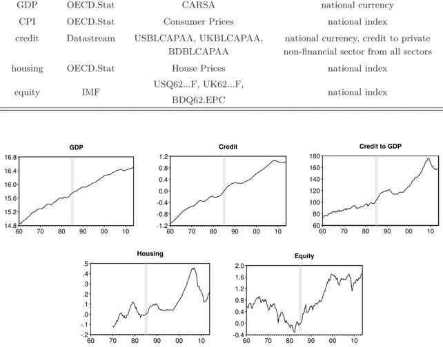
Appendix A Data Sources and Definitions
All series are measured in logs and deflated using the consumer price index. All series are normalized by their respective value in 1985Q1 to ensure comparability of the units. We obtain annual growth rates by taking annual differences of the time series. The only exception is the credit to GDP ratio which is expressed in percentage points.
Table 6: Definition and Sources of the Data
Source Identifier Notes
GDP OECD.Stat CARSA national currency
CPI OECD.Stat Consumer Prices national index
credit Datastream USBLCAPAA, UKBLCAPAA, national currency, credit to private BDBLCAPAA non-financial sector from all sectors
housing OECD.Stat House Prices national index
equity IMF USQ62...F, UK62...F,
BDQ62.EPC national index
14.8 15.2 15.6 16.0 16.4 16.8
60 70 80 90 00 10
GDP
-1.2 -0.8 -0.4 0.0 0.4 0.8 1.2
60 70 80 90 00 10
Credit
60 80 100 120 140 160 180
60 70 80 90 00 10
Credit to GDP
-.2 -.1 .0 .1 .2 .3 .4 .5
60 70 80 90 00 10
Housing
-0.4 0.0 0.4 0.8 1.2 1.6 2.0
60 70 80 90 00 10
Equity
Figure 7: Real GDP and Financial Cycle Proxy Variables in the United States. All series are log levels excepting the credit to GDP ratio, which represents in percentage points. The vertical gray line shows the sample split.
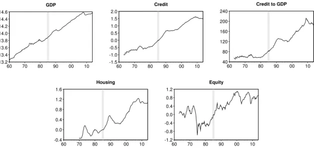
13.2 13.4 13.6 13.8 14.0 14.2 14.4 14.6
60 70 80 90 00 10
GDP
-1.5 -1.0 -0.5 0.0 0.5 1.0 1.5 2.0
60 70 80 90 00 10
Credit
40 80 120 160 200 240
60 70 80 90 00 10
Credit to GDP
-0.4 0.0 0.4 0.8 1.2 1.6
60 70 80 90 00 10
Housing
-1.2 -0.8 -0.4 0.0 0.4 0.8 1.2
60 70 80 90 00 10
Equity
Figure 8: Real GDP and Financial Cycle Proxy Variables in the United Kingdom. All series are log levels excepting the credit to GDP ratio, which represents in percentage points. The vertical gray line shows the sample split.
13.4 13.6 13.8 14.0 14.2 14.4 14.6 14.8 15.0
60 70 80 90 00 10
GDP
-1.6 -1.2 -0.8 -0.4 0.0 0.4 0.8
60 70 80 90 00 10
Credit
50 60 70 80 90 100 110 120 130 140
60 70 80 90 00 10
Credit to GDP
-.24 -.20 -.16 -.12 -.08 -.04 .00 .04 .08 .12 .16
60 70 80 90 00 10
Housing
-0.8 -0.4 0.0 0.4 0.8 1.2 1.6
60 70 80 90 00 10
Equity
Figure 9: Real GDP and Financial Cycle Proxy Variables in Germany. All series are log levels excepting the credit to GDP ratio, which represents in percentage points. The vertical gray line shows the sample split.