Ecology and Evolution. 2018;1–9. www.ecolevol.org | 1
1 | INTRODUCTION
In this time and era where many organisms are facing great environ‐
mental challenges, the need to evaluate the demographics of animal
populations to guide conservation and management practices is high and rising. Mortality rates are among the most important de‐
mographic parameters for understanding population dynamics (Caughley, 1977). Probably, the most widely used methodologies to Received: 6 April 2018
|
Revised: 13 October 2018|
Accepted: 29 November 2018DOI: 10.1002/ece3.4854
O R I G I N A L R E S E A R C H
The adequacy of aging techniques in vertebrates for rapid
estimation of population mortality rates from age distributions
Meijuan Zhao
1,2| Chris A. J. Klaassen
3| Simeon Lisovski
2,4| Marcel Klaassen
2This is an open access article under the terms of the Creative Commons Attribution License, which permits use, distribution and reproduction in any medium, provided the original work is properly cited.
© 2018 The Authors. Ecology and Evolution published by John Wiley & Sons Ltd.
1School of Life Sciences, University of Science and Technology of China, Hefei, Anhui, China
2Centre for Integrative Ecology, School of Life and Environmental Sciences, Deakin University, Geelong, Victoria, Australia
3Korteweg‐de Vries Institute for Mathematics, University of Amsterdam, Amsterdam, The Netherlands
4Swiss Ornithological Institute, Department of Bird Migration, Sempach, Switzerland Correspondence
Meijuan Zhao, School of Life Sciences, University of Science and Technology of China, Hefei, Anhui, China.
Email: meijuanzhao1@gmail.com
Abstract
As a key parameter in population dynamics, mortality rates are frequently estimated using mark–recapture data, which requires extensive, long‐term data sets. As a po‐
tential rapid alternative, we can measure variables correlated to age, allowing the compilation of population age distributions, from which mortality rates can be de‐
rived. However, most studies employing such techniques have ignored their inherent inaccuracy and have thereby failed to provide reliable mortality estimates. In this study, we present a general statistical model linking birth rate, mortality rate, and population age distributions. We next assessed the reliability and data needs (i.e., sample size) for estimating mortality rate of eight different aging techniques. The results revealed that for half of the aging techniques, correlations with age varied considerably, translating into highly variable accuracies when used to estimate mor‐
tality rate from age distributions. Telomere length is generally not sufficiently corre‐
lated to age to provide reliable mortality rate estimates. DNA methylation, signal‐joint T‐cell recombination excision circle (sjTREC), and racemization are generally more promising techniques to ultimately estimate mortality rate, if a sufficiently high sam‐
ple size is available. Otolith ring counts, otolithometry, and age‐length keys in fish, and skeletochronology in reptiles, mammals, and amphibians, outperformed all other aging techniques and generated relatively accurate mortality rate estimation with a sample size that can be feasibly obtained. Provided the method chosen is minimizing and estimating the error in age estimation, it is possible to accurately estimate mor‐
tality rates from age distributions. The method therewith has the potential to esti‐
mate a critical, population dynamic parameter to inform conservation efforts within a limited time frame as opposed to mark–recapture analyses.
K E Y W O R D S
age estimation, aging error, birth rate, demographics, mark–recapture, survival rate
assess mortality rates in populations are mark–recapture analyses.
However, mark–recapture analyses tend to require large and long‐
term data sets. For instantaneous, snapshot estimation of mortality rates, age distributions within populations serve as an alternative and a series of models have been developed to that effect (Supporting information Appendix S1). A cited reference search for these models and refining by “age” in combination with “mortality” or “survival”
in Web of Knowledge yielded 2065 studies (date accessed on 10 October 2018), implying the wide application of deducing mortal‐
ity rate from age distribution. Although this approach bears notable promises for cases where urgent assessment of population status is required, there has thus far been little consideration of its accuracy involving a robust statistical approach.
Almost invariably the underlying age distributions used in the calculation of mortality rates are subject to error. Although various models assessed mortality rates from age distributions (Supporting information Appendix S1), all but Conn, Doherty, Nichols, Ricklefs, and Rohwer (2005) assumed that age was estimated without error.
Thus, the reliability of deduced mortality rates was generally over‐
rated. Conn et al. (2005) used only two age categories, that is, ju‐
venile and adult, numerically investigating the consequences of misclassification to these two categories. Their study pointed out that substantial errors in mortality rate estimation can potentially be made using this approach even if other major assumptions, such as that the age distribution across the population under study is sta‐
ble, are being met. Despite its critical importance, a robust statistical model to investigate the propagation of errors in age estimation to mortality rate estimates from age distributions has, to our knowl‐
edge, not previously been developed.
Birth and survival processes determine the age distribution within a population. The birth and survival distributions over time are therefore intimately linked with a population’s age distribution.
Provided that the age distribution of a population can be measured, and the birth distribution of that population is known, the survival distribution can be estimated, and vice versa. Birth distributions can often be assessed with much more ease than survival distributions or can alternatively be reasonably assumed (e.g., a uniform distribu‐
tion; that is, a constant average birth rate; Ball, Britton, & Trapman, 2017; Thornley & France, 2016). The interest therefore primarily lies with being able to reliably estimate a survival distribution from a population’s age distribution.
Our study has three aims that are being addressed in separate sections of the paper: (a) To provide a detailed statistical description of the relationship between a population’s birth rate, survival rate, and age distributions, we present a statistical model for the analyti‐
cal derivation of mortality rates and their confidence intervals from age distributions, taking errors in age estimation into account. (b) To evaluate the accuracy of different aging techniques in determining age, we next reviewed the accuracy of a range of popular or po‐
tentially promising aging techniques employed in vertebrates. These include measurement of telomere length, DNA methylation, sig‐
nal‐joint T‐cell recombination excision circle (sjTREC), racemization, otolith ring counts, otolithometry (measurement of otolith mass,
length, width, and height), age‐length keys, and skeletochronology.
(c) Finally, we used our statistical model to evaluate the suitability of these aging techniques to accurately estimate mortality rates.
2 | MATERIALS AND METHODS
2.1 | Model description
We here provide a brief outline of the statistical models that are pre‐
sented in more detail, including all assumptions made, in Supporting information Appendix S2. To facilitate cross‐referencing between the below and Supporting information Appendix S2, we retain equa‐
tion numbers as used is Supporting information Appendix S2.
Consider a well‐defined population for which we want to evalu‐
ate its dynamics and potentially simulate or predict its future devel‐
opment. The development of this population is necessarily stochastic and is determined by the survival function 1−FS(s) and the birth time density function fT(t) of its members, ultimately resulting in the pop‐
ulation’s age density function fY(y). Here, the subscripts S, T and Y denote the survival time, the time of birth, and the age, respectively, of a random individual from the population. Furthermore, we follow the convention of indicating distribution functions by F and proba‐
bility density functions by f. The relationship between these three entities, survival time, time of birth, and age, is given by formula
or equivalently.
Given two of these three entities, the third one is determined.
In the majority of cases, fT(t) can be assessed in some way or rea‐
sonably assumed. Consequently, an estimate of the survival function 1−FS(s), which is of key interest, can be computed via Equation (), provided fY(y) can be estimated.
To obtain an estimate of fY(y), one has to measure the age of individuals from a population directly. However, this is almost always impossible and one consequently has to rely on measuring other variables, so‐called age proxies X, that correlate strongly with age Y. In Supporting information Appendix S2, statistical solutions are provided for the case where a single (d = 1) or multiple (d > 1) age proxies X are described as a function of age Y. In the framework of the current study where we wish to review the suitability of spe‐
cific age proxies in isolation, we specifically consider the case d = 1 with X = X(1), a one‐dimensional age proxy. For d = 1, we assume that there exists a strictly monotone, known function g(y), a known pos‐
itive constant σ, and a random variable ε with known density f𝜀(z), distribution function F𝜀(z), mean E𝜀=0, and variance E𝜀2=1, such that
(3) fY(y) =
(1−FS(y)) fT(−y)
∫0∞( 1−FS(t))
fT(−t)dt, − ∞<y<∞,
(4) 1−FS(s) = fT(
0) fY(s) fT(−s)fY(
0), − ∞<s<∞.
X=g( (8) Y)
+𝜎𝜀
which ultimately (see Supporting information Appendix S2) yields:
Furthermore, for the specific aims of our study we make the clas‐
sic assumption that the monotone function g(y) is linear, that is, that there exist known constants α and β with
Thus, the dependence of the age proxy X on the age Y is de‐
scribed via linear regression with normal error.
As outlined in Supporting information Appendix S2, we need not necessarily make any assumptions on the class of survival functions 1−FS(s) and resort to a so‐called nonparametric estimation prob‐
lem to estimate the density function fX(x). However, in such cases estimating the density function fY(y) is a so‐called deconvolution problem, which is notoriously hard to solve. For these problems, convergence rates in n (i.e., the number of age proxies measured) are extremely slow, like √
lnn; see Carroll and Hall (1988). On the other hand, if restriction of the survival function to a parametric class of survival functions is justified, estimation of the survival function at a
√n rate becomes feasible.
To satisfy the wish for a parametric class of survival functions, we may consider an exponential distribution for the survival time S of a newborn (chosen at random) from a population. This means that we assume the existence of a positive number 𝜆 with.
and 𝜆= −ln( 1−m)
, which implies that the density of S satisfies
Loosely speaking, m is the probability that an individual dies within the next time unit. Therefore, m is called the mortality rate and 0<m<1 holds.
Although this simplification, which assumes a constant mortality rate m with age, is not strictly necessary from a mathematical per‐
spective (i.e., models allowing for much more general or complex relationships between survival and age, and thus mortality rate and age, are feasible as outlined above and in Section 3 of Supporting information Appendix S2), it dramatically reduces the required sam‐
ple size. In many cases, this is also a reasonable assumption for two reasons. Firstly, some species do show either a constant mortality rate or a roughly constant mortality rate before reaching a very ad‐
vanced age (6 out of 23 vertebrates investigated in Jones et al., 2014).
Secondly, although in the remaining species the relationship between age and mortality rate varies, it often increases exponentially with age, resulting in few individuals within wildlife populations living long enough to be impacted by a substantially increased mortality rate with age. Hence, estimating age‐specific mortality rates often require
large, long‐term data sets, be it mark–recapture data or population age distribution data. Such data are, however, available for very few species only (Jones et al., 2014). Most case studies lack sufficient data and thus estimate mortality rate based on the assumption of a con‐
stant adult mortality. Given the relatively low number of individuals affected by advanced‐age‐related changes in mortality, the potential impact on the population dynamics of such assumption may also be limited. Finally, this simplification is notably warranted in the present case, where the aim of the exercise is primarily focused on evaluating the suitability of a range of popular or potentially promising verte‐
brate aging techniques to establish population age distributions with the purpose of estimating survival functions.
Next to the value of the age proxy X of sampled individuals, one might be able to observe additional information about these individ‐
uals, like their sex and other characteristics. In principle, such covari‐
ates might help in obtaining a more precise estimate of the true age Y.
However, given the limited availability of such data in the literature, we will not pursue this approach any further in this paper.
To simplify further, we assume that the population is completely stable, in the sense that fT(t) is the uniform density on [−𝜏,0] with 𝜏 tending to infinity. In view of Equations () and (), we have
This means that the age Y of an arbitrary individual from the pop‐
ulation has the same exponential distribution as the survival time S of a newborn. Next, combination of Equations (10) and (18) shows that the density of the age proxy X becomes.
Writing 𝜇=𝜎𝜆∕|𝛽| we note that estimation of the mortality rate
is equivalent to estimation of the parameter 𝜇, which we propose to call proxy coefficient. With Φ (z) denoting the standard normal distribution function, Equation (20) can be rewritten in terms of 𝜇 as
The correlation between the age Y and the age proxy X equals 1/√
1+𝜇2. So, the smaller the proxy coefficient 𝜇, the larger the cor‐
relation between the age and the age proxy.
To estimate the value of m or equivalently of 𝜇= −𝜎(ln(1−m))
|𝛽| (cf.
Equation ), we take a random sample of size n from the population and determine the values of age‐correlated variable X of the selected individuals. Let us denote these values as x1,…,xn, which are viewed as realizations of the independent random variables X1,…,Xn, with density from Equation (23).
fX(x) = (10)
∞∫
0
1 𝜎f𝜀
(x−g( Y) 𝜎
) fY(y)dy.
(19) g(y) =𝛼+𝛽y, y>0.
(15) 1−FS,𝜆(s) =P(S>s)=e−𝜆s=(1−m)s, s≥0,
(16) fS,𝜆(s) =𝜆e−𝜆s, s≥0.
(18) fY,𝜆(y) = 1−FS,𝜆(y)
�0∞(
1−FS,𝜆(t)) dt=e−𝜆y
1∕𝜆=𝜆e−𝜆y, y≥0.
(20) fX,𝜆(x) =
∞∫
0
1 𝜎𝜑
(x−𝛼−𝛽y 𝜎
)
𝜆e−𝜆ydy, x∈ℝ.
(22) m=1−exp(−𝜆) =1−exp(−|𝛽|𝜇∕𝜎)
(23) fX,𝜆(x) =𝜇
𝜎exp (1
2𝜇2−𝜇 𝛽
|𝛽| x−𝛼
𝜎 )
Φ ( 𝛽
|𝛽| x−𝛼
𝜎 −𝜇 )
.
In Supporting information Appendix S2, it is shown that the Fisher information for proxy coefficient 𝜇equals.
and that the asymptotically efficient estimator 𝜇̂n of 𝜇 can be de‐
fined as
with 𝜑/Φ (z) written as short hand for 𝜑(z)/Φ (z). “Asymptotically efficient” means that the estimator has approximately a normal dis‐
tribution for large sample sizes n with the true value 𝜇 as mean and the smallest possible variance, namely nJ(𝜇)1 .
In view of Equations (15) and (22), the corresponding efficient estimator m̂n for m equals.
By taking many samples of size n from the set of numbers {x1,…,xn }, computing the corresponding estimates of m, and estimating in this
way the distribution of m̂n,we may construct a bootstrap confidence interval for m.
As an alternative 95% confidence interval for m, we mention.
where the function.
is evaluated at m̂n.Here, J(𝜇)is as in Equation (32) and I(m)is the Fisher information for m. The 95% confidence range (CR) may be cal‐
culated by deducting the lower limit from the upper limit and equals
We define the empirical 95% error percentage as.
which estimates the theoretical 95% error percentage.
with m the true value of the mortality rate. We used EEP(95) to as‐
sess the accuracy of mortality rate estimation from age distributions with large values indicating high variation and thus lower accuracy.
2.2 | Review of aging techniques
To obtain a general impression of the performance of each aging tech‐
nique when assessing mortality rate using age distributions, we re‐
viewed eight aging techniques for vertebrates including measurement of telomere length, DNA methylation, sjTREC, racemization, otolith ring count, otolithometry, age‐length keys, and skeletochronology.
These eight aging techniques were reviewed because they are well‐
known indicators that to some extent correlate with age (i.e., telomere length, otolith ring count, otolithometry, age‐length keys, and skel‐
etochronology) or are promising indicators in determining age with low errors (i.e., DNA methylation, sjTREC, and racemization). We reviewed these techniques in terms of the animal classes to which they have been applied, their accuracy in predicting age and factors other than age (e.g., environmental factors, health status) influencing their suitabil‐
ity as age estimators (background details of the eight aging techniques are presented in Supporting information Appendix S3). To evaluate their accuracy as age predictors in vertebrates, we selected 218 data points from 123 case studies, extracted the relationship between age (32)
J(𝜇) = 1
𝜇2−1−𝜇2+𝜇∫
∞
−∞
𝜑(z)
Φ (z)𝜑(z+𝜇)dz
̂ (36) 𝜇n= (
1+1 Ĵn
)
̄ 𝜇n− 1
n̂Jn
∑n i=1
𝜑 Φ
( 𝛽
|𝛽| Xi−𝛼
𝜎 −𝜇̄n )
(37) m̂n=1−exp
(
−|𝛽|𝜇̂n 𝜎
) .
(39)
⎡⎢
⎢⎢
⎣
m̂n− 1.96
� n I�
m̂n�, m̂n+ 1.96
� n I�
m̂n�
⎤⎥
⎥⎥
⎦ ,
(38) I(m) =
𝜎2J(
−𝜎
|𝛽| ln( 1−m)) 𝛽2(1−m)2
CR( (42) 95)
= 3.92
√ nI(
m̂n).
EEP� (43) 95�
=CR� 95�
m̂n ×100%= 392
√n
× 1
m̂n
� I�
m̂n� %,
(44) EP�
95�
= 392
√n × 1
m√ I(m)
%, FI G U R E 1 Lookup plot for the basic factor in the error percentage.
Lookup plot for 1
m√
I(m), the basic factor in the error percentage EP(95) (calculated as the 95% confidence range divided by the expected mortality rate m using Equation for various combinations of mortality rate (m; y‐axis) and aging parameter (|𝛽∕𝜎|; x‐axis). 𝛽 and 𝜎 represent the slope and standard deviation of the error in a linear regression of age against age markers estimated by different aging techniques, respectively. The absolute value of 𝛽∕𝜎, |𝛽∕𝜎|, is the key variable representing the accuracy of aging techniques in the estimation of age and thus the estimation of mortality rate. Shadings range from black (poor performance) via gray to white (good performance), where black shading on the left‐hand corner indicates combinations of m and |𝛽∕𝜎| which yield proxy coefficient μ > 8. For such cases, 1
m√
I(m) is large and the computation of its exact value is unreliable. We thus considered techniques yielding low |𝛽∕𝜎| values that result in μ > 8 as performing very poorly and unable to accurately estimate mortality rate.
estimators and true age, and obtained𝛽∕𝜎 the crucial indicator for the variation in estimated mortality rate (see Equations and ) and the R2 for each study (data are presented in Supporting information Appendix S4). Specifically, we conducted a Web of Knowledge search using the key words “age estimation” or “age determination” or “age assessment”
or “estimat* age” or “assign* age” combined with the name of each aging technique. From these studies and the relevant studies cited therein, we selected only those investigating long‐lived (maximum age esti‐
mated ≥2 years) vertebrates, with a sample size larger than five, includ‐
ing both laboratory‐ and field‐based studies. Moreover, we excluded cases investigating the correlation of age proxy and real age in diseased individuals. Only a small proportion of these studies provided raw data that we could directly use to calculate R2 and 𝛽∕𝜎. In the remaining cases where only data distributions were provided, we used bootstrap‐
ping over 10,000 iterations to generate data and subsequently calcu‐
late a mean R2 and 𝛽∕𝜎. To evaluate the performance of the various aging techniques within animal classes, for each of these groups the median and range of R2 and 𝛽∕𝜎 were calculated.
To evaluate the performance of the reviewed aging techniques when assessing mortality rate using age distributions, we constructed a lookup plot (Figure 1) for 1
m√
I(m),the basic factor in the 95% error per‐
centage EP(95) (see Equation (44) with the absolute value of 𝛽∕𝜎 or |𝛽∕𝜎| ranging from 0.01 to 75 (range of observed |𝛽∕𝜎|, the upper limit 75 is the second largest observed value of|𝛽∕𝜎|, the largest value infinite) and the mortality rate m ranging from 0.01 to 0.99. Using Equation (44), we also constructed a lookup table (Table 1) to assist determining the min‐
imum sample size n required to estimate mortality rate with a specific accuracy (i.e., with a desired 95% error percentage EP(95)) for various combinations of |𝛽∕𝜎| and expected mortality rate m.
3 | RESULTS
In our statistical approach, the accuracy of the aging technique |𝛽∕𝜎|, the sample size n, and the expected mortality rate m are the three de‐
terminant parameters for the variation in the estimated mortality rate.
m
|β/σ|
0.1 0.2 0.5 1 2 5 10
EP (95) = 5% 0.1 9,813 6,682 5,738 5,584 5,542 5,530 5,528
0.2 23,431 9,150 5,650 5,105 4,953 4,907 4,900
0.3 51,048 14,055 5,821 4,690 4,376 4,278 4,263
0.4 90,927 22,168 6,244 4,321 3,806 3,644 3,618
0.5 139,059 33,378 6,935 3,981 3,238 3,005 2,967
EP (95) = 10% 0.1 2,454 1671 1,435 1,396 1,386 1,383 1,382
0.2 5,858 2,288 1,413 1,277 1,239 1,227 1,225
0.3 12,762 3,514 1,456 1,173 1,094 1,070 1,066
0.4 22,732 5,542 1561 1,081 952 911 905
0.5 34,765 8,345 1734 996 810 752 742
EP (95) = 20% 0.1 614 418 359 349 347 346 346
0.2 1,465 572 354 320 310 307 307
0.3 3,191 879 364 294 274 268 267
0.4 5,683 1,386 391 271 238 228 227
0.5 8,692 2087 434 249 203 188 186
EP (95) = 30% 0.1 273 186 160 156 154 154 154
0.2 651 255 157 142 138 137 137
0.3 1,418 391 162 131 122 119 119
0.4 2,526 616 174 121 106 102 101
0.5 3,863 928 193 111 90 84 83
EP (95) = 40% 0.1 154 105 90 88 87 87 87
0.2 367 143 89 80 78 77 77
0.3 798 220 91 74 69 67 67
0.4 1,421 347 98 68 60 57 57
0.5 2,173 522 109 63 51 47 47
Notes. 𝛽 and 𝜎 represent the slope and the standard deviation of the error in a linear regression of age against age markers estimatedy different aging techniques, respectively. The absolute value of 𝛽∕𝜎,
|𝛽∕𝜎|,is the key variable representing the accuracy of aging techniques in the estimation of age and thus in the estimation of mortality rate.
TA B L E 1 The minimum number of individuals required to estimate mortality rate with a specific accuracy (i.e., the 95%
error percentage EP (95)) for various combinations of |𝛽∕𝜎| and expected mortality rate m
In Figure 1, we translated the simultaneous variations in |𝛽∕𝜎| and m into the variation in the basic factor (i.e., 1
m√
I(m)) that correlates posi‐
tively with the error percentage EP(95) (Equation ). This factor, and thus EP(95), generally decreases with an increase in |𝛽∕𝜎|. However, in the range of 0.2 <|𝛽∕𝜎|<2, the basic factor decreases rapidly after which the basic factor changes little for |𝛽∕𝜎|>2, plateauing around
|𝛽∕𝜎|= 5.
An interaction exists between |𝛽∕𝜎|and m. When |𝛽∕𝜎|>0.5, the basic factor generally decreases with an increase in m, meaning that for a certain sample size the accuracy of an aging technique should increase when m decreases in order to keep EP(
95) stable. However, when |𝛽∕𝜎| <0.5, the basic factor and thus EP(95) increase rather than decrease with m. When mortality rate m tends to be high, and
|𝛽∕𝜎| tends to be low, the 𝜇 in Equation (22) is high. For large 𝜇 values, for example, 𝜇>8, the basic factor in EP(95) is high, but the compu‐
tation of its exact value is numerically unreliable, due to the division of two extremely small numbers in element 𝜇∫−∞∞ 𝜙(z)
Φ(z)𝜙(z+𝜇)dz in Equation (i.e., in the computation of J, which is subsequently used in Equations and ). We thus considered aging techniques yielding low
|𝛽∕𝜎| values that result in μ > 8 as performing very poorly and unable to accurately estimate mortality rate. We like to stress that Equation (44) and hence Figure 1 and its properties sketched here are conse‐
quences of the model we have chosen via Equations (15) and (19).
Table 1 shows the minimum sample size n needed for a suffi‐
ciently accurate estimate of mortality rate. When the aging tech‐
nique performs poorly, that is,|𝛽∕𝜎| is low, the required sample size n to achieve a low EP(95) is large. For instance, more than 400 indi‐
viduals are required to achieve an EP(95) of 20% when |𝛽∕𝜎| < 0.2.
Whether or not such a high sample size is difficult to achieve very much depends on the ease of obtaining animals for aging, which may be species and context dependent, and the (costs of the) methods involved in estimating age. Yet, it is clear that one should generally strive for the use of aging techniques with |𝛽∕𝜎|>0.2 when estimating mortality rate is one of the ultimate targets.
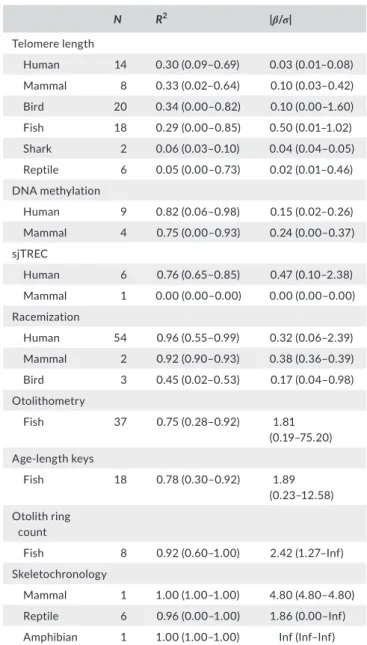
The eight aging techniques achieved highly different accuracies in terms of their R2 and |𝛽∕𝜎| (Table 2). Telomere length invariably yielded poor matches. On average, DNA methylation, sjTREC, and racemization performed slightly better. Otolithometry, age‐length keys, otolith ring count, and skeletochronology tended to provide the best outcomes. However, all aging techniques showed markedly different performances across taxa and studies with even the most promising techniques, otolith ring count and skeletochronology, oc‐
casionally proved to be unreliable.
Although showing a relatively good correlation with age in some fish studies, telomere length seems to be a generally poor proxy for age. In many studies, telomere length did not correlate with age and the median R2 across taxa was <0.35. With the exception of fishes, in most cases |𝛽∕𝜎| < 0.2 (Table 2), indicating that the method is not suf‐
ficiently adequate to estimate mortality rate from age distributions.
DNA methylation performed slightly better than telomere length, with a median R2 across taxa between 0.75 and 0.85. Although the median |𝛽∕𝜎| in mammals was just above 0.2, |𝛽∕𝜎| varied consider‐
ably across studies and was incidentally as low as 0 (Table 2).
sjTREC in humans performed slightly better than DNA methyl‐
ation, with a median |𝛽∕𝜎| of 0.47 (Table 2). However, the single ap‐
plication of sjTREC in mammals showed no correlation with age (Ito, Yoshimura, & Momoi, 2015).
TA B L E 2 Summary of accuracy in aging across studies employing eight different aging techniques for a range of vertebrate taxa
N R2 |β/σ|
Telomere length
Human 14 0.30 (0.09–0.69) 0.03 (0.01–0.08) Mammal 8 0.33 (0.02–0.64) 0.10 (0.03–0.42)
Bird 20 0.34 (0.00–0.82) 0.10 (0.00–1.60)
Fish 18 0.29 (0.00–0.85) 0.50 (0.01–1.02)
Shark 2 0.06 (0.03–0.10) 0.04 (0.04–0.05)
Reptile 6 0.05 (0.00–0.73) 0.02 (0.01–0.46) DNA methylation
Human 9 0.82 (0.06–0.98) 0.15 (0.02–0.26)
Mammal 4 0.75 (0.00–0.93) 0.24 (0.00–0.37) sjTREC
Human 6 0.76 (0.65–0.85) 0.47 (0.10–2.38)
Mammal 1 0.00 (0.00–0.00) 0.00 (0.00–0.00) Racemization
Human 54 0.96 (0.55–0.99) 0.32 (0.06–2.39) Mammal 2 0.92 (0.90–0.93) 0.38 (0.36–0.39)
Bird 3 0.45 (0.02–0.53) 0.17 (0.04–0.98)
Otolithometry
Fish 37 0.75 (0.28–0.92) 1.81
(0.19–75.20) Age‐length keys
Fish 18 0.78 (0.30–0.92) 1.89
(0.23–12.58) Otolith ring
count
Fish 8 0.92 (0.60–1.00) 2.42 (1.27–Inf)
Skeletochronology
Mammal 1 1.00 (1.00–1.00) 4.80 (4.80–4.80) Reptile 6 0.96 (0.00–1.00) 1.86 (0.00–Inf) Amphibian 1 1.00 (1.00–1.00) Inf (Inf–Inf) Notes. N, number of case studies; R2, 𝛽,and 𝜎 represent the coefficient of determination, the slope, and the standard deviation of the error in a linear regression of age against age markers estimated by different aging techniques, respectively. The absolute value of 𝛽∕𝜎, |𝛽∕𝜎|,is the key vari‐
able representing the accuracy of aging techniques in the estimation of age and thus in the estimation of mortality rate. Humans considered separate from other mammals. N, median, and range for R2 and |𝛽∕𝜎| are provided for each taxon. Individual data for all case studies are provided in Supporting information Appendix S4.
sjTREC means signal‐joint T‐cell recombination excision circles; accura‐
cies of otolithometry and age‐length keys are probably inflated since these used otolith ring counts to assess true age without validation; Inf indicates infinite |𝛽∕𝜎| for σ = 0, that is, no error in age determination.
Racemization performed similarly to DNA methylation and sjTREC with considerable variation within and between taxa. A num‐
ber of racemization studies in humans and mammals achieved a me‐
dian R2 > 0.9 and a median|𝛽∕𝜎| > 0.2. The R2 and |𝛽∕𝜎| of individual studies, however, could be as low as those found in studies employ‐
ing telomere length (Figure 2 and Table 2). Moreover, to date its ap‐
plication to nonhuman vertebrates has been highly limited (Table 2).
Otolith ring counts, which are limited to studies in fish, showed best correlations with age, with a median R2 and |𝛽∕𝜎| of 0.9 and 2.4, respectively (Table 2). This is therewith the only technique achieving a median |𝛽∕𝜎| higher than 2. One study even scored a 100% ac‐
curacy (Gooley, 1992). Both otolithometry and age‐length keys, for which we found studies in fish exclusively although indeterminate growth is also present in reptiles and amphibians, could likewise pro‐
vide good estimates of age, with |𝛽∕𝜎| close to 2. It should be noted that in all these studies where age was based on otolith ring counts, this age was considered to be the true age and that our estimates of accuracy for these studies are thus potentially inflated.
Albeit sample size was limited to one in both taxa, the (near) 100% accuracy for skeletochronology in amphibians (Friedl & Klump, 1997) and mammals (Castanet et al., 2004) indicates great promise for this technique (Table 2). This promise was supported by the larger sample of reptile studies yielding |β/σ| close to 2 (Table 2).
4 | DISCUSSION
Despite their wide use to this effect, half of the aging techniques reviewed were not sufficiently reliable to invariably yield satisfyingly
accurate mortality rate estimates, for populations with a roughly con‐
stant mortality rate during adulthood. Telomere length performed worst; the two molecular methods, DNA methylation and sjTREC, and the chemical method, racemization, perform slightly better. The two techniques that can exclusively be used in fish (i.e., otolith ring count and otolithometry) and two techniques with potential wider application, that is, age‐length keys and skeletochronology, per‐
formed best. If we would consider error percentages ≤20% at an assumed mortality rate of the population of 0.3 as sufficiently ac‐
curate, |𝛽∕𝜎| would have to be higher than 0.34 when n = 500. Under this scenario, only 31% of the case studies using telomere length resulted in sufficiently accurate mortality rate estimates. This pro‐
portion increased to 62% in studies using DNA methylation, sjTREC, or racemization; 75% in skeletochronology; and increased to 92% in studies using otolith ring count, otolithometry, or age‐length keys.
Thus, any application of these aging techniques for mortality rate es‐
timates would need to carefully evaluate the error in age estimation and should not take high accuracies in age estimation for granted.
Finally, one could also resort to measuring and combining multiple age proxies to estimate age and therewith reduce error and improve accuracy. In Supporting information Appendix S2 Section 2, the sta‐
tistical basis for this approach is provided.
Although not explicitly addressed in our review since the ex‐
amples are few, we noted that the performances of some aging techniques varied considerably between populations, genders, and tissues examined, for example, between populations using otolith‐
ometry (Newman, 2002), genders using age‐length keys (Ordines, Valls, & Gouraguine, 2012), and tissues using telomere length (Izzo, 2010). Thus, in addition to using multiple age proxies, the inclusion F I G U R E 2 Performance of the reviewed aging techniques. Box plots displaying the variations within and among the reviewed aging techniques (Supporting information Appendix S3) in their correlations with age in terms of |𝛽∕𝜎|. 𝛽 and 𝜎 represent the slope and the standard deviation of the error in a linear regression of age against age markers estimated by different aging techniques, respectively.
The absolute value of 𝛽∕𝜎, |𝛽∕𝜎|, is the key variable representing the accuracy of aging techniques in the estimation of age and thus in the estimation of mortality rate. Aging techniques along the x‐axis are ranked in order of increasing median |𝛽∕𝜎| across case studies. Numbers along the top of the panel denote number of case studies. The thick line within each box and whisker plot represents the median, and the lower and upper box border represent the first and the third quartile, respectively. Whiskers denote the lower and upper 95% confidence interval. Dots outside the whiskers are outliers above or below the 95% confidence interval.
of covariates in the estimation of age from age proxies may be an additional avenue to improve accuracy.
Telomere length has been one of the first molecular indicators that were found to correlate with age. However, it was far from satisfying to allow for its use in “mortality rate from age distribu‐
tion modeling,” consistent to the conclusion by Dunshea et al.
(2011) that telomere length is insufficiently accurate to estimate age in vertebrates. The aging techniques here reviewed are among the most promising or popular ones. In fish, growth ring counts in other hard structures, such as scales, vertebrae, and fins, have also been employed in age estimation but have generally been found to be less accurate than otolith ring counts (e.g., Vandergoot, Bur, &
Powell, 2008, Ma, Xie, Huo, Yang, & Li, 2011). Other morphologi‐
cal measurements and molecular biomarkers have also been used in vertebrates. For instance, measurement of shoulder height in el‐
ephant (Shrader et al., 2006); pentosidine in many mammalian spe‐
cies (Brownlee, Vlassara, Kooney, Ulrich, & Cerami, 1986; Sell et al., 1996) and poultry (Iqbal, Probert, & Klandorf, 1997); and lipofuscin in fishes (Girven, Gauldie, Czochanska, & Woolhouse, 1993) and hu‐
mans (Goyal, 1982). However, all these techniques were less accu‐
rate than the reviewed alternatives, especially at older age, and were thus not included in our review.
Besides the accuracy of aging techniques in terms of |𝛽∕𝜎|, sam‐
pling effort also plays a key role in the accuracy of mortality esti‐
mates. For populations with an expected m lower than 0.5, to obtain a mortality estimate with an error percentage under 20%, one has to sample a large number of individuals, for example, >400 when |𝛽∕𝜎| is below 0.2. Sampling effort under 180 individuals in this case can never achieve such proposed accuracy. Therefore, a combination of a reliable aging technique and a large sample size is crucial to obtain an accurate mortality estimate.
Although estimation of mortality rate from population age distri‐
butions has been widely applied, our model is the first to assess the accuracy of age distribution‐based mortality rate by taking errors in aging into consideration using a robust statistical model. The model makes a set of assumptions (see Section 4 of Supporting information Appendix S2) of which two are particularly noteworthy: (1) that the population is stable in the survival function of its individuals and (2) that mortality rate is constant across age groups. Fortunately, for as‐
sumption (1) to hold, the population need not be stable in numbers, but only in its age distribution. Nevertheless, we highlight that it should be realized that such age distributions are the result of popu‐
lation dynamic processes over time, including variations therein. The model assumes that such variations do not exist. If these variations do exist, as in wild populations, it will not detriment the performance of the model if those variations distribute around a mean and do not vary with age or time; such possibilities need to be considered in the interpretation of the model’s outcomes. As outlined in Materials and methods and Supporting information Appendix S2, assumption 2 is not a prerequisite to allow estimation of mortality rates from age dis‐
tributions taking errors in age proxies into consideration. However, assuming a constant mortality rate across age groups greatly reduces sample size requirements (to √
n; Supporting information Appendix
S2), which is of great importance considering the still large sample sizes required using this simplifying assumption. Admittedly, a con‐
stant mortality rate with age does not conform with reality in a range of species. For vertebrates where this has been investigated in detail, it applied to 6 out of 23 species (Jones et al., 2014). Nevertheless, it is an importantly simplifying assumption that is frequently adopted in initial analyses of population dynamics, especially for populations under threat with a lack of historical data to derive an age‐specific mortality rate. Moreover, depending on the nature of mortality–
age relationships, of which many different forms exist (Jones et al., 2014), deviations from a roughly constant mortality rate with age may only occur at a highly advanced age and apply to a small, poten‐
tially negligible fraction of the population only. Such deviations from constant mortality rate may also hold for immatures, which in many species can be easily identified and removed from the analysis. Our statistical model thus serves as a first step before considering more complex alternatives, which will either require considerably larger data sets or, if resorting to mark–recapture, large longitudinal data sets. Irrespectively, we emphasize that while our specific model does not account for potential differential mortality rates with age, it still provides a good impression on how errors in aging translate into er‐
rors in mortality rate estimation.
The specific model here presented is applicable to any proxy for age that has, or can be converted to, a linear relationship with age.
The application of the model to the reviewed data highlights that a relatively accurate aging technique and large sampling effort are needed to yield reliable mortality rate estimates. However, as op‐
posed to mark–recapture studies, the method still has great poten‐
tial for conservation efforts where time is at a premium, allowing the estimation of mortality rate as a crucial population dynamic parame‐
ter within a limited period of time.
CONFLIC T OF INTEREST None declared.
AUTHOR CONTRIBUTION
MK and MZ conceived the ideas; CK, MK, and MZ designed method‐
ology; MZ collected the data; MZ and SL analyzed the data; MZ and MK led the writing of the main manuscript; and CK led the writing of Supporting information Appendix S2. All authors contributed criti‐
cally to the drafts and gave final approval for publication.
DATA ACCESSIBILIT Y
R2 and |β/σ| for case studies employing eight different aging tech‐
niques will be archived in Dryad Digital Repository should the manu‐
script be accepted.
ORCID
Meijuan Zhao https://orcid.org/0000‐0001‐9625‐1821
REFERENCES
Ball, F., Britton, T., & Trapman, P. (2017). An epidemic in a dynamic popu‐
lation with importation of infectives. The Annals of Applied Probability, 27, 242–274.
Brownlee, M., Vlassara, H., Kooney, A., Ulrich, P., & Cerami, A. (1986).
Aminoguanidine prevents diabetes‐Induced arterial‐wall protein cross‐linking. Science, 232, 1629–1632.
Carroll, R. J., & Hall, P. (1988). Optimal rates of convergence for decon‐
volving a density. Journal of the American Statistical Association, 83, 1184–1186.
Castanet, J., Croci, S., Aujard, F., Perret, M., Cubo, J., & de Margerie, E.
(2004). Lines of arrested growth in bone and age estimation in a small primate: Microcebus murinus. Journal of Zoology, 263, 31–39.
Caughley, G. (Ed.) (1977). Analysis of vertebrate populations. New York, NY: John Wiley & Sons.
Conn, P. B., Doherty, P. F., Nichols, J. D., Ricklefs, R. E., & Rohwer, S.
(2005). Comparative demography of New World populations of thrushes (Turdus spp.): Comment. Ecology, 86, 2536–2544. https://
doi.org/10.1890/04‐1799
Dunshea, G., Duffield, D., Gales, N., Hindell, M., Wells, R. S., & Jarman, S.
N. (2011). Telomeres as age markers in vertebrate molecular ecology.
Molecular Ecology Resources, 11, 225–235.
Friedl, T. W., & Klump, G. M. (1997). Some aspects of population biology in the European treefrog, Hyla arborea. Hyla Arborea. Herpetologica, 321–330.
Girven, R. J., Gauldie, R. W., Czochanska, Z., & Woolhouse, A. D. (1993).
A test of the lipofuscin technique of age estimation in fish. Journal of Applied Ichthyology‐Zeitschrift Fur Angewandte Ichthyologie, 9, 82–88.
Gooley, G. J. (1992). Validation of the use of otoliths to determine the age and growth of Murray cod, Maccullochella peelii (Mitchell) (Percichthyidae), in Lake Charlegrark, western Victoria. Australian Journal of Marine & Freshwater Research, 43, 1091–1102.
Goyal, V. K. (1982). Lipofuscin pigment accumulation in human brain during aging. Experimental Gerontology, 17, 481–487.
Iqbal, M., Probert, L. L., & Klandorf, H. (1997). Effect of dietary amino‐
guanidine on tissue pentosidine and reproductive performance in broiler breeder hens. Poultry Science, 76, 1574–1579.
Ito, G., Yoshimura, K., & Momoi, Y. (2015). Gene analysis of signal‐joint T cell receptor excision circles and their relationship to age in dogs.
Veterinary Immunology and Immunopathology, 166, 1–7.
Izzo, C. (2010). Patterns of telomere length change with age in aquatic ver‐
tebrates and the phylogenetic distribution of the pattern among jawed vertebrates. PhD thesis. Adelaide, SA: University of Adelaide.
Jones, O. R., Scheuerlein, A., Salguero‐Gomez, R., Camarda, C. G., Schaible, R., Casper, B. B., … Vaupel, J. W. (2014). Diversity of ageing across the tree of life. Nature, 505, 169–173.
Ma, B., Xie, C., Huo, B., Yang, X., & Li, P. (2011). Age validation, and comparison of otolith, vertebra and opercular bone for estimating age of Schizothorax o’connori in the Yarlung Tsangpo River, Tibet.
Environmental Biology of Fishes, 90, 159–169.
Newman, S. J. (2002). Growth rate, age determination, natural mortal‐
ity and production potential of the scarlet seaperch, Lutjanus mal‐
abaricus Schneider 1801, off the Pilbara coast of north‐western Australia. Fisheries Research, 58, 215–225. https://doi.org/10.1016/
S0165‐7836(01)00367‐8
Ordines, F., Valls, M., & Gouraguine, A. (2012). Biology, feeding, and habitat preferences of Cadenat’s rockfish, Scorpaena loppei (Actinopterygii: Scorpaeniformes: Scorpaenidae), in the Balearic Islands (western Mediterranean). Acta Ichthyologica Et Piscatoria, 42, 21–30.
Sell, D. R., Lane, M. A., Johnson, W. A., Masoro, E. J., Mock, O. B., Reiser, K. M., … Monnier, V. M. (1996). Longevity and the genetic determi‐
nation of collagen glycoxidation kinetics in mammalian senescence.
Proceedings of the National Academy of Sciences of the United States of America, 93, 485–490.
Shrader, A. M., Ferreira, S. M., McElveen, M. E., Lee, P. C., Moss, C. J.,
& van Aarde, R. J. (2006). Growth and age determination of African savanna elephants. Journal of Zoology, 270, 40–48.
Thornley, J. H., & France, J. (2016). Blue tongue–A modelling examina‐
tion of fundamentals–Seasonality and chaos. Journal of Theoretical Biology, 403, 17–29.
Vandergoot, C. S., Bur, M. T., & Powell, K. A. (2008). Lake erie yellow perch age estimation based on three structures: Precision, process‐
ing times, and management implications. North American Journal of Fisheries Management, 28, 563–571.
SUPPORTING INFORMATION
Additional supporting information may be found online in the Supporting Information section at the end of the article.
How to cite this article: Zhao M, Klaassen CAJ, Lisovski S, Klaassen M. The adequacy of aging techniques in vertebrates for rapid estimation of population mortality rates from age distributions. Ecol Evol. 2018;00:1–9. https://doi.
org/10.1002/ece3.4854