Small Area Estimation of Poverty in Rural Bhutan
Technical Report jointly prepared by National Statistics Bureau of Bhutan and the World Bank June 21, 2010
National Statistics Bureau Royal Government of Bhutan
South Asia Region Economic Policy and Poverty The World Bank
68179
Public Disclosure AuthorizedPublic Disclosure AuthorizedPublic Disclosure AuthorizedPublic Disclosure Authorized
1
Acknowledgements
The small area estimation of poverty in rural Bhutan was carried out jointly by National Statistics Bureau (NSB) of Bhutan and a World Bank team – Nobuo Yoshida, Aphichoke Kotikula (co-TTLs) and Faizuddin Ahmed (ETC, SASEP). This report summarizes findings of detailed technical analysis conducted to ensure the quality of the final poverty maps. Faizuddin Ahmed contributed greatly to the poverty estimation, and Uwe Deichman (Sr. Environmental Specialist, DECEE) provided useful inputs on GIS analysis and creation of market accessibility indicators. The team also acknowledges Nimanthi Attapattu (Program Assistant, SASEP) for formatting and editing this document.
This report benefits greatly from guidance and inputs from Kuenga Tshering (Director of NSB), Phub Sangay (Offtg. Head of Survey/Data Processing Division), and Dawa Tshering (Project Coordinator).
Also, Nima Deki Sherpa (ICT Technical Associate) and Tshering Choden (Asst. ICT Officer) contributed to this analysis, particularly at the stage of data preparation, and Cheku Dorji (Sr. Statistical Officer) helped to prepare the executive summary and edited this document.
The team would like to acknowledge valuable comments and suggestions from Pasang Dorji (Sr.
Planning Officer) of the Gross National Happiness Commission (GNHC) and from participants in the poverty mapping workshops held in September and December 2009 in Thimphu. This report also benefits from the feasibility study conducted on Small Area Estimation of poverty by the World Food Program in Bhutan.
Finally, the team would like to thank Nicholas J. Krafft (Country Director for Bhutan) and Miria Pigato (Sector Manager of SASEP) for their generous and continued support for this analysis and the preparation of this report.
2
ABBREVIATIONS, ACRONYMS, AND GLOSSARY
BLSS Bhutan Living Standard Survey MDGs Millennium Development Goals
dzongkhag District NSB National Statistics Bureau
ELL Elbers et al. RGOB Royal Government of Bhutan
gewog Sub-district SAE Small Area Estimation
GIS Geographical Information System WDR World Development Report (WDR) GNHC Gross National Happiness
Commission
WFP World Food Program
3
Table of Contents
Executive Summary ... 4
Section I: Introduction ... 5
Section II: Poverty Mapping Method ... 6
Methodology ... 6
Main Data Sources ... 7
Technical Challenges ... 8
Production of Poverty Maps and Quality Checks ... 9
Section III: Poverty Mapping Results ... 16
Poverty Headcount Rate vs. Number of Poor Population ... 17
Poverty maps with other geo-referenced data ... 18
(i) Market Accessiblity and Poverty ... 18
(ii) Access to Education and Poverty ... 19
(iii) Electrification and Poverty ... 19
(iv) Gender and Poverty ... 20
Section IV: Conclusion ... 21
Caveats ... 21
Poverty Mapping as a Regular Monitoring Instrument ... 21
Combining Poverty Maps with Geographical Database ... 21
References ... 23
Annex I: Results of Rural Poverty Map ... 24
Annex II: Results of Consumption Models ... 29
Annex III: Accessibility Indicators ... 33
Annex IV: Descriptions of national poverty line, specifics of BLSS data, and Census ... 35
Annex V: Standard errors and statistically distinguishable rankings ... 37
4
Executive Summary
The Small Area Estimation (SAE) of Poverty in Rural Bhutan was prepared with an objective to provide a more disaggregated picture of poverty in Bhutan down to the gewog level, based on the Bhutan Living Standard Survey (BLSS) 2007 and Population & Housing Census of Bhutan (PHCB) 2005.
The analysis was carried out by the National Statistics Bureau (NSB) and the World Bank in response to the emerging need of the Royal Government of Bhutan (RGOB) especially for effective resource allocation to all the gewogs.
The report records the estimation process in detail and describes results of statistical tests for quality checks. According to these tests, the poverty estimates at the gewog level are reliable. The report also enhances the transparency of the process and intends to serve as a guide for future updates.
According to the Poverty Analysis Report (PAR) 2007, about one-fourth of the country’s population is estimated to be poor with rural poverty as high as 30.9 percent. It also shows that poverty rates are high in Zhemgang, Samtse, Monggar and Lhuntse dzongkhags. This report, which presents some results of the SAE, compliments the PAR 2007 by further identifying pockets of poverty in these dzongkhags as well as in other dzongkhags
The results from the SAE are compared with other geo-referenced database. It is observed that, generally poor gewogs tend to have limited access to markets and road networks. Similarly, access to rural electrification is relatively low in poor areas while densely populated but non-poor gewogs in Paro, Chukha, Thimphu and Punakha have high rates of rural electrification. Furthermore, the poverty incidence of each gewog is highly associated with school attendance of children. For example, poor gewogs register lower school attendance compared with non-poor gewogs. As such, overlaying a poverty map with other geo-referenced indicators is highly informative, and some of these findings can be used for designing, planning and monitoring poverty alleviation strategies at the gewog level.
5
Section I: Introduction
1. Over the past 10 years, Bhutan has performed remarkably well in reducing poverty. However, vast differences in poverty levels across dzongkhag (district) and gewog (sub-district) persist. Popular perceptions suggest that the geography of poverty and of economic affluence is accentuated at the local level, and that an understanding of the spatial distribution of economic welfare is needed in order to spread the benefits of growth to lagging regions. In order to fulfill Bhutan’s development philosophy of gross national happiness, and poverty reduction, it is essential to understand its geographic and spatial patterns. In the case of Bhutan, its land-locked geography and sparse population pose major challenges for poverty reduction. Poverty maps will help the government and development partners locate pockets of poverty which might otherwise be overlooked.
2. The Royal Government of Bhutan (RGOB) is committed to carrying out various programs to alleviate poverty and deprivation, and to achieve the Millennium Development Goals (MDGs).
Although many of these programs are centrally funded, they are frequently carried out at dzongkhag and gewog levels. However, limited data on poverty and other key human development indicators at the sub- national levels constrain the local and central governments’ capability to monitor spending and outcomes. As asserted in the 10th Five Year plan, allocating resources to poor gewog is essential to assisting them tackling their residents’ poverty.
3. Precise poverty estimates at the gewog level will facilitate the implementation of the newly- introduced, formula-based mechanism for resource allocation from the central government to all gewogs.
Previously, in the absence of poverty maps, all gewogs in a dzongkhag were assumed to have equal poverty rates. However, following the preparation of the new poverty maps, the block grants can now incorporate gewog-level poverty estimates to better reflect ground-level realities. Using poverty maps and other geographic data, local governments can identify key development bottlenecks for their constituencies.
4. The Poverty Mapping was implemented to largely help fill the data gap. It combines existing census and survey data, and produces reliable poverty estimates at lower levels of disaggregation than existing survey data would permit. A more disaggregated picture below the district may help uncover pockets of poverty and deprivation that might otherwise be overlooked, thereby potentially informing the design of targeted interventions. Performance monitoring could also be improved with the availability of poverty maps that permit the tracking of poverty at the local level over multiple time periods.1 Overlaying a poverty map with other geo-referenced information such as transport infrastructure, public service centers, and information on natural resources, like soil quality, may also help identify the investments necessary to lift such areas out of poverty. Market access maps are examples of this geographical database.
5. In response to the demand from the RGOB, the National Statistics Bureau (NSB) and the World Bank, with support from the Gross National Happiness Commission (GNHC), launched the Small Area Estimation initiative, or so-called Poverty Mapping, in December 2008. A technical working group was formed, comprised of staff members from the NSB, the GNHC, and the World Bank. This task benefited greatly from a feasibility study completed by the World Food Program (WFP) and NSB. In June 2009, the working group discussed the preliminary results and provided comments and suggestions to the World Bank team. After a review by technical committee, the task was completed in September 2009.
1 An immediate use of a poverty map in India would be to monitor the 200 districts identified as backward areas for implementation of an employment guarantee scheme. Through this scheme, the Government intends to create village-level assets generating future employment and improving other welfare indicators in these regions.
6
The poverty maps at the gewog level will be an effective tool in allocating resources to the target population, enabling not only efficient use of the scarce resources but also carrying out direct interventions to the poor.
6. The Bhutan Poverty Mapping applied a Small Area Estimation (SAE) method developed by Elbers et al. (2003); this methodology has been widely tested and applied around the world. The Elbers et al. approach was carefully implemented in the present project, and considerable efforts were made to avoid or minimize potential bias.
7. Capacity-building has been a very important component of this task; its aim is to ensure that poverty mapping can be used as a regular monitoring instrument. To support this objective, the World Bank provided multiple rounds of training on poverty mapping methodology to the staff from the RGOB. The World Bank’s new software, PovMap2, was actively utilized in the estimation process as well as in training sessions. Several staff members from the NSB and the GNHC have actively participated in the training sessions in Bhutan and Bangladesh, to understand and learn the methodology and software used for poverty mapping.
8. The structure of this report is as follows. Section II describes the poverty mapping method, particularly the SAE method and comprehensive detail of validation and quality checks of poverty mapping results. Section III illustrates the results. Section IV shows some uses of poverty maps with other geo-referenced datasets. Section V lists concluding remarks. Technical discussion of other related topics are presented in the Technical Annex I.
Section II: Poverty Mapping Method
9. Historically, poverty has been measured by using sample survey consumption data, in which household per capita expenditures are compared against a poverty line. Under this approach the sampling error of poverty estimates rises rapidly as the target area gets smaller. It therefore precludes analysts from estimating poverty at a disaggregated level.
10. In order to estimate poverty at a disaggregated level, the Bhutan team selected the Small Area Estimation method developed by Elbers et al. (2003) (henceforth referred to as ELL). This method uses the strengths of both the 2005 Population Census and the 2007 BLSS to produce statistically reliable poverty estimates at the gewog level. In contrast, traditional approaches of poverty estimation cannot produce reliable estimates below the dzongkhag level because these would yield large sampling errors.
Methodology
11. Many poverty mapping methodologies have been proposed in the literature (see for example, Bigman and Deichmann, 2000). These methods have their respective advantages and disadvantages, but recently the ELL method has been gaining popularity among development practitioners worldwide.
12. As mentioned above, the Bhutan poverty mapping applies the ELL methodology. In the ELL method, consumption levels are imputed for each household in the population census based on a consumption model estimated from a household survey. The consumption model must include explanatory variables (household and individual characteristics) that are available in both the census and the survey. By applying estimated coefficients to these same variables in the census data, consumption expenditures can be imputed to each census household. Poverty and inequality statistics for small areas can then be calculated based on this imputed per capita consumption for each census households.
13. One advantage of the ELL method is that it not only sets out to estimate poverty incidence, but also yields estimates of standard errors on the poverty estimates. Since such poverty estimates are
7
computed based on imputed consumption, they are clearly subject to imputation errors, which are reflected in the standard errors.
14. The standard errors are helpful in guiding analysts about the precision and reliability of the poverty estimates produced with the ELL methodology. In their original studies, Elbers et al. (2002, 2003) analyze the properties of the imputation errors in detail and derive a procedure to compute standard errors of poverty estimates.
Main Data Sources
15. The primary data sources used in the ELL methodology are household survey and population census data. The Bhutan Poverty Mapping uses unit record data from the PHCB 2005 and the BLSS 2007.. As a common practice throughout the world, the Census does not include information on household consumption and income levels. The BLSS, on the other hand, contains detailed information on consumption as well as a wealth of additional information on employment, ownership of assets, housing condition, and access to services such as education and health. This large set of variables is a key to the procedure of imputing household consumption from the survey into the population census.
Most variables from BLSS are representative at the dzongkhag level. The BLSS was collected by the NSB in 2007 (March-May), while the Census reference date was May 31, 2005.2
2 See more details in Annex IV.
Box 1: The Small Area Estimation method developed by ELL (2003)
The method proposed by ELL has two stages. In the first stage, a model of log per capita consumption expenditures (lnych) is estimated in the survey data:
ch ch
ch X Z u
y ln
where
Xch is the vector of explanatory variables for household h in cluster c, is the vector of associated regression coefficients, Z is the vector of location specific variables with being the associated vector of coefficients, and uch is the regression disturbances due to the discrepancy between the predicted household consumption and the actual value. This disturbance term is decomposed into two independent components:
ch c
uch with a cluster-specific effect,c, and a household-specific effect,ch. This error structure allows for both a location effect—common to all households in the same area—and heteroskedasticity in the household-specific errors. The location variables can be at any level of disaggregation—district, gewog, or chiwog—and can be drawn from any data source that includes all the locations in the country. All parameters regarding the regression coefficients (, ) and distributions of the disturbance terms are estimated by Feasible Generalized Least Square (FGLS). In the second part of the analysis, poverty estimates and their standard errors are computed. There are two sources of errors involved in the estimation process: errors in the estimated regression coefficients (ˆ, ˆ) and the disturbance terms, both of which affect poverty estimates and the level of their accuracy. ELL propose a way to properly calculate poverty estimates as well as measure their standard errors while taking into account these sources of bias. A simulated value of expenditures for each census household is calculated with predicted log expenditures XchˆZˆ and random draws from the estimated distributions of the disturbance terms, c and ch. These simulations are repeated 100 times. For any given location (such as a dzongkhag or a gewog), the mean across the 100 simulations of a poverty statistic provides a point estimate of the statistic, and the standard deviation provides an estimate of the standard error.
8 Technical Challenges
16. The ELL poverty mapping methodology continues to evolve in response to ongoing scrutiny from researchers. To this end, a variety of documents and manuals are available on the World Bank website to inform practitioners of the latest developments and methodological improvements of the SAE method. These improvements are also reflected in the updated versions of the PovMap2 software produced by the World Bank to assist with application of the procedure.
17. The present Bhutan Poverty Mapping faced two main technical challenges: (i) an interval between the PHCB 2005 and the BLSS 2007 and (ii) the Tarrozi and Deaton (2008) critique.
Interval between PHCB 2005 and BLSS 2007
18. The Poverty Mapping Methodology is founded on a consumption model estimated using the BLSS 2007 data, in which household per capita expenditure is regressed on a set of household and individual characteristics. As described earlier, information on these characteristics is available in both the BLSS 2007 and PHCB 2005. It then predicts household expenditure into each census household based on the model.
19. The appeal of this approach is most obvious if the PHCB 2005 reflects the situation of BLSS 2007 well. This assumption is reasonable given the short interval and the seemingly limited change in the socio-economic structure of Bhutan during the period. Moreover, both datasets were collected or referenced at the same time of year. However, it might be possible that consumption patterns changed markedly between the period as a result of structural changes and relative price shifts. The population distribution might also have changed due to migration. Changes in consumption patterns and the population distribution can introduce biases in the poverty estimates and their standard errors derived from the ELL method.3
Misspecifications of Consumption Models and Error Structures
20. In a recently published paper, Tarozzi and Deaton (2008) highlight a number of concerns with the ELL methodology that can be summarized as follows.
21. First, differences in consumption patterns within a domain can bias both poverty estimates and the standard errors. The ELL method estimates a consumption model that is assumed to apply to all households within each domain (in the case of Bhutan poverty mapping: large urban, small urban, and rural areas). The implicit assumption is that the relationship between household expenditures and its correlates is the same for all households within the domain, and that all remaining differences are due not to structural factors, but are attributable to errors. This is not a minor assumption and is explicitly acknowledged as such in ELL (2003).
22. Second, misspecification in the error structure can lead to an overstatement of the precision of resultant poverty estimates. In its current configuration, PovMap2, the software developed by the World Bank for the purpose of poverty mapping (freely downloadable from www.iresearch.worldbank.org), can accommodate only two layers of errors: at the level of the household and at the level of some unit of aggregation above the household. In the case of the present study, the two layers of errors were selected
3 One way to reduce this risk is to focus on common variables that did not change much over time. Such an approach was adopted in Bangladesh, and was found to be effective in reducing bias. This approach is certainly worth being tested in the future.
9
to be households and the sample clusters (corresponding to “chiwogs”4 in rural areas and “towns” in urban areas). However, as noted by Tarozzi and Deaton (2008), there could be correlation in errors also at some higher level, such as the gewog level, which is above the chiwog and below the district level (or districts and town/cities in urban areas), and a further correlation can exist at the district level. Tarozzi and Deaton (2008) show that if the ELL method is applied and any existing correlation of errors at these higher levels of aggregation is ignored, then standard errors on poverty estimates can be understated – resulting in an overly optimistic assessment of the precision of the poverty estimates. One apparent solution to this issue is to allow for more than two layers of errors in implementation of the ELL methodology. This, however, is not a feasible solution given the sampling design of most household surveys, including the BLSS.
23. The poverty mapping procedure comprises two main components: (i) selecting sound consumption models and (ii) selecting the level of disaggregation.
24. The explanatory power of the consumption models that were estimated for the Bhutan Poverty Mapping Project was generally quite high. In addition, the unexplained variation in household consumption at the cluster level (chiwog for rural areas and city/town for urban areas) appears moderate.
These two observations combine to suggest that there is limited scope for the kind of concerns raised by Tarozzi and Deaton (2008). Nonetheless, the issues are real and must be tackled. It is reassuring that district level poverty rates estimated from this exercise match those estimated directly from the BLSS 2007 data.
25. In Bhutan, the primary objective of this exercise was to produce poverty estimates at the gewog level for rural areas, and at the town level for urban areas. The report carefully assessed the quality of the poverty estimates that were produced, and concluded that rural poverty maps were sufficiently accurate, while urban poverty maps were not as reliable. This section also explains how the challenges pointed out by Tarrozi and Deaton (2008) were addressed. This section goes on to explain how the levels of disaggregation for producing poverty maps – gewog level for rural areas and district level for urban areas – were selected. Final models are listed in Table A-3 of Annex 1.
Model Selection
26. The Bhutan Poverty Mapping exercise prepared three different consumption models; large urban cities, small/medium sized cities/towns, and rural areas.
27. As mentioned earlier, failure to capture regional differences in consumption patterns could bias poverty estimates produced with the ELL method. Regional differences in consumption pattern can often be substantial. For example, the educational attainment of household heads might be a good predictor of household wealth in urban areas, whereas it might not be as important in rural areas, where the agricultural sector dominates.
28. Despite potential heterogeneity across areas, increasing the number of consumption models does not necessarily improve the statistical performance of poverty mapping. As the number of models rises,
4 Chiwog is commonly translated as “block”. It is an administrative level that lies below gewog but above village. It usually compose of a few villages.
10
the sample size in the BLSS 2007 data for each model declines, lowering the accuracy and stability of the consumption model.
29. In order to find a balance between capturing regional heterogeneity and maintaining adequate sample sizes it was decided to create three consumption models (large urban, small urban, and rural areas). Urban areas were split to two domains – large cities and small/medium cities after confirming consumption models of these areas are statistically different.
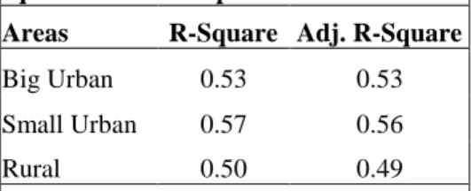
30. The accuracy of poverty estimates depends on the predictive power of consumption models.
This predictive power is gauged by R-squared statistics. Both R-squared and Adjusted R-squared statistics provide information on how well a consumption model can predict the actual consumption expenditure of each census household. Specifically, the R-squared is a statistic that indicates how well the predicted expenditure from a consumption model fits the actual household expenditure. The higher the R-squared, the better the predicted expenditure fits the actual household expenditure. Adjusted R- squared is a modification of R-squared that adjusts for the number of regressors in a model. R-squared always increases when a new variable is added to a model, but adjusted R-squared increases only if the new variable improves the model more than would be expected by chance.
31. The consumption models, generally, only capture part of the variation in household expenditures, and the unexplained variation is called residuals
(or simply errors). The residuals can be separated into two layers in the present analysis – the household layer and the cluster layer (“chiwog” in rural areas and “town/city” for urban areas). The cluster effect is included since consumption expenditures can be affected by region- specific factors that are common across households, some of which may be observable while others are not.
32. Since residual location effects such as cluster effects
can reduce the precision of poverty and inequality estimates, Elbers et al. (2002, 2003) recommend applying great effort to capturing variation in consumption by observables as far as possible. If chiwog level error is large, reliability of poverty estimates is low. A rule of thumb is to reduce the share of the variance of the cluster effect to the total variance of residuals to 10 percent or lower. International experience suggests that in rural areas achievement of this goal often remains elusive (see Mistiaen et al., 2002).
33. A strategy for reducing the share of the variance of the cluster effect is to include location- specific variables in the regression models. In the case of the Bhutan Poverty Mapping, the team uses location-specific variables that can be constructed by aggregating data from the Population Census. Such effort has been found to be of great importance also in addressing the concerns raised by Tarozzi and Deaton (2008) regarding the precision of poverty map estimates.
34. The exercise reveals that the error structure is judicious and effects of cluster variance are at minimum. The share of the variance of the cluster effect to the total variance of residuals in the small urban model is 9 percent and in the rural model 12 percent. Judging by the rule of thumb mentioned above, there is still room for improvement for the rural consumption model.
Table 1: R-squared and Adjusted R- squared of consumption models
Areas R-Square Adj. R-Square
Big Urban 0.53 0.53
Small Urban 0.57 0.56
Rural 0.50 0.49
Source: Authors’ estimation
11 35. Datasets used for the Bhutan Poverty Mapping have three layers of administrative units that are below the district level: gewog; chiwog, and village (or town/city). Consumption models in the Bhutan Poverty Mapping can control for correlation of errors at the district level, since consumption models include district dummies. However, controlling for correlations at the gewog level, as well as the chiwog level, was not possible.
36. As mentioned above, if the variance of errors at the gewog level were high relative to the overall variance, then ignoring the gewog-level error
could lead to a significant underestimation of standard errors (Tarrozi and Deaton, 2007).
Elbers et al. (2008) show that if location- specific variables are included in consumption models (particularly at the level of the gewog), the risk of underestimating the standard errors of poverty estimates may be attenuated. The Bhutan Poverty Mapping follows this strategy in specifying the consumption models.
37. Elbers et al. (2008) also propose tests to assess the likelihood of underestimated standard errors of poverty estimates. One approach is to switch the location effect from the cluster level (chiwog) to the gewog level and to then examine by how much standard errors rise. Switching the location effect from a smaller unit to a larger unit tends to increase standard errors of poverty estimates. Because in reality correlation of
errors would likely occur at both the gewog and chiwog levels, assuming that the entire effect occurs at the gewog level would thus likely exaggerate the size of standard errors. The true level of standard errors of poverty estimates must be somewhere in between.
38. Indeed, standard errors rise significantly after switching the level of cluster effect from chiwog to gewog. Table 2 shows how many times the standard errors increase as a result of switching the cluster from chiwog to gewog. Irrespective of which is chosen, mean or median, the standard error more than doubles after switching the cluster level from chiwog to gewog.
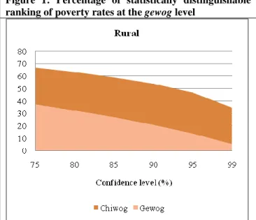
Figure 1: Percentage of statistically distinguishable ranking of poverty rates at the gewog level
Source: Authors’ estimation, using BLSS 2007 and Population Census 2005.
Table 2: Comparison on mean and median of Standard Errors of poverty estimates at the gewog level if the cluster level is changed
Cluster level Mean Median
chiwog 0.032 0.035
gewog 0.072 0.083
Ratio (gewog/chiwog) 2.3 2.4 Source: Authors’ estimation
Table 3: Variances of different layers Domain
Two-layer model One-layer model
Gewog chiwog Household All chiwog Household All
1: Rural 5.00 8.00 87.00 100.00 12.00 88.00 100.00
2: Large Urban Not available convergence not achieved
3: Small Urban Not available 9.00 91.00 100.00
Source: World Bank staff estimations using BLSS 2007 and PHCB 2005. Chiwog is the administrative level that only applicable in rural areas; therefore, this switching analysis was not conducted for the urban case.
12
39. Unsurprisingly, the share of statistically distinguishable rankings among gewogs falls if the cluster is shifted from chiwog to gewog, particularly in rural areas (see Figure 1 above). For example, in rural areas, when the cluster effect and the confidence level are set at the chiwog level and at 75 percent respectively, nearly 70 percent of gewogs can be ranked with statistical significance. However, if the cluster effect is defined to apply at the gewog level, the percentage falls to less than 40 percent. In urban areas, ignoring correlations at the gewog level is far less problematic. The share of statistically distinguishable rankings among gewogs does not fall much in urban areas.
40. The above test is thus able to provide some reassurance that standard errors reported here for urban areas are reasonable. However, in rural areas, the standard errors reported here could well be overly optimistic. In a further effort to probe whether the location effect should, in fact, be more reasonably applied at the gewog level in rural areas than at the cluster level, Elbers et al. (2008) propose another test, based on a mixed-maximum likelihood procedure (STATA command XTMIXED), that allows more than two layers of errors. Here the idea is to explicitly examine what fraction of the location effect occurs at the cluster level, and what fraction at the gewog level.
41. Contributions of gewog, chiwog, and household level errors were estimated for each stratum separately using this STATA command (see Table 3). There is a case for which the procedure could not converge, and for which results are thus not available. Non-convergence seems to occur more frequently if the consumption model includes a large number of explanatory variables, particularly dummy variables.
42. In rural and small urban areas, the contribution of gewog-level errors was found to be quite limited: the variance of the gewog-level errors constituted no more than five percent of variance of the total errors. The results indicate that most errors apply at the chiwog and the household levels, and these are explicitly taken into account by the PovMap2 software.
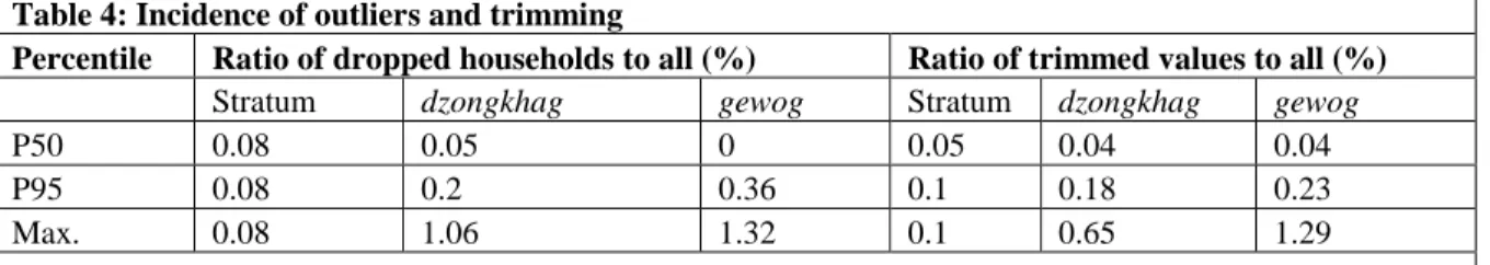
43. Another set of important modeling issues is confronted when handling outliers in the simulated household expenditures of census households. The ELL method simulates household expenditure for all census households by randomly drawing parameters (including both regression coefficients and residuals) from their corresponding distributions, as estimated in the survey-based consumption model.
One issue with this method is that random drawing can potentially pick extreme values, albeit with low probability. Simulated household expenditures can thus include a few outlier values. PovMap2 allows for the elimination of such outliers by dropping them before estimating poverty and inequality indicators.
Such an adjustment, which is often called ‘trimming,’ is needed since a few outliers can produce huge biases, especially in inequality statistics. However, trimming is more of a practical solution than one derived from rigorous statistical theory. In this sense, it would always be preferable if a consumption model could be specified from which a need for trimming did not arise.
Table 4: Incidence of outliers and trimming
Percentile Ratio of dropped households to all (%) Ratio of trimmed values to all (%)
Stratum dzongkhag gewog Stratum dzongkhag gewog
P50 0.08 0.05 0 0.05 0.04 0.04
P95 0.08 0.2 0.36 0.1 0.18 0.23
Max. 0.08 1.06 1.32 0.1 0.65 1.29
Source: World Bank staff estimations using BLSS 2007 and PHCB 2005.
13
44. Table 4 summarizes the incidence of trimming at three different administrative unit levels if the final consumption models were adopted. It shows that all strata, districts, and gewogs (or towns in urban areas) involve a very low incidence of trimming. Such results are encouraging, since such outliers can bias poverty estimates.
The Level of Disaggregation
45. As noted above, the ELL method produces standard errors of poverty estimates, which can be useful to practitioners in finding the appropriate level of disaggregation of poverty estimates. Although most statistics of this type are associated with certain margins of error, results of poverty mapping are frequently reported without providing any information about such errors. PovMap2 provides both poverty estimates and their standard errors.
46. Table 5 shows that most standard errors are of
reasonable size. For example, a median of standard errors at the gewog level is 4.6 percentage points in rural areas, which means the 95 percent confidence interval of the corresponding poverty estimate has a range of only +/- 9 percentage points from the poverty estimate. Even the 95th percentile of standard errors is 7.4 percentage points. The performance at higher levels of aggregation is even better: the maximum standard error is nearly 15 percentage points, which is admittedly large. However, this is only the case when the standard error is beyond 10 percent – all other poverty estimates have less than 10 percentage points of standard error.
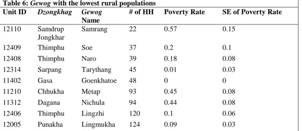
47. However, in comparison to other countries’ poverty mapping, Bhutan’s poverty estimates have slightly higher standard errors. In Bangladesh, the 95th percentile of all standard errors at the Upazila level is at 4 percentage points, while in India the 99th percentile of all standard errors at the Tehsil level is at 7 percentage points. The fact that some gewogs have few households is likely to contribute to the higher standard errors than other countries. The gewog with low number of households are shown below,
and Table 6 shows the 10 least populated gewog in Bhutan.
Table 5: Accuracy of poverty estimates (standard error at the Gewog level, %)
Median 95% Max
urban 1.9 6.6 8.4 rural 4.6 7.4 14.8
Source: World Bank staff estimations using BLSS 2007 and PHCB 2005.
Table 6: Gewog with the lowest rural populations Unit ID Dzongkhag Gewog
Name
# of HH Poverty Rate SE of Poverty Rate 12110 Samdrup
Jongkhar
Samrang 22 0.57 0.15
12409 Thimphu Soe 37 0.2 0.1
12408 Thimphu Naro 39 0.18 0.08
12314 Sarpang Tarythang 45 0.01 0.03
11402 Gasa Goenkhatoe 48 0 0
11210 Chhukha Metap 93 0.45 0.08
11312 Dagana Nichula 94 0.44 0.08
12406 Thimphu Lingzhi 120 0.1 0.06
12005 Punakha Lingmukha 124 0.09 0.03
Source: World Bank staff estimations using BLSS 2007 and PHCB 2005.
14
Ranking gewogs with Poverty Estimates from the Bhutan Poverty Mapping 48. The most relevant feature of the poverty map in
policy-making is its ability to rank gewog by their poverty rates. Such a feature allows policy-makers to prioritize and allocate resources to address the overall poverty reduction policies. Therefore, it is important to study the extent that we can rank gewogs according to poverty estimates from the Bhutan Poverty Mapping.
49. Overall, the standard errors of rural poverty estimates at the gewog level are low enough to yield a statistically significant ranking. The ability to rank poverty across towns is limited in urban areas.
50. Ranking of true poverty incidence can be different from ranking of poverty estimates. Figure 2 shows the percentage of rankings based on poverty mapping by level of statistical significance. The result suggests that rural poverty
maps were sufficiently accurate, while urban poverty maps were not as reliable.5 Consistency with Poverty Rates Directly Estimated from the BLSS 2007 51. The reliability of
estimates from the ELL method can be verified by comparing with the corresponding numbers estimated directly from the BLSS 2007 data. Key variables in the BLSS 2007 data are representative at the dzongkhag (district) level, separately for urban and rural areas. The ELL method can obviously generate estimates at the dzongkhag level as well. Presumably, if underlying assumptions of within-region homogeneity and of relative stability between 2005 and 2007 do not hold, there would be little reason to expect estimates based on the ELL method to
5 See Annex V for more details.
Figure 2: Percentage of statistical significant ranking of gewogs in poverty
Source: World Bank staff estimations using BLSS 2007 and PHCB 2005.
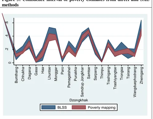
Figure 3: Confidence interval of poverty estimates from direct and SAE methods
0.2.4.6 Bumthang Chhukha Dagana Gasa Haa Lhuntse Monggar Paro Pemagatshel Punakha Samdrup Jongkhar Samtse Sarpang Thimpu Trashigang Trashiyangtse Trongsa Tsirang Wangduephodrang Zhemgang
Dzongkhak
BLSS Poverty mapping
Source: World Bank staff estimations using BLSS 2007 and PHCB 2005
15
be close to those from the BLSS data directly. Conversely, if the ELL method produces a good predictor of true poverty incidence, this should be consistent with that estimated from BLSS 2007 data.
52. Consistency checks are applied using the 95 percent confidence intervals of both estimates. Both poverty estimates are statistics rather than true levels, and their 95 confidence intervals reflect the margins of errors of the poverty estimates. These two estimates can be considered as consistent if the 95 percent confidence intervals are overlapping.
53. Figure 3 shows dzongkhag-level poverty rates from poverty mapping and compares them with the official poverty rates from BLSS 2007. The blue band indicates a range where a true poverty rate exists with a probability of 95 % according to BLSS 2007 estimates. The red band indicates the range according to the poverty mapping. For example, for Dagana, the BLSS 2007 estimate suggests the true poverty rate is likely located somewhere between 20 and 40 percent, while poverty mapping suggests it is likely located between 25 and 35 percent.
54. Two observations emerge. First, these two bands are overlapping, which means that predictions of true poverty rates from both BLSS 2007 and poverty mapping are consistent. Second, the red band is smaller than the blue one, indicating that poverty mapping can locate the level of true poverty rates more accurately. This reflects the fact that estimates directly from the BLSS 2007 survey are based on far fewer data points than are those based on the PHCB 2005.
Sensitivity check: Is the poverty map sensitive to choice of poverty line?
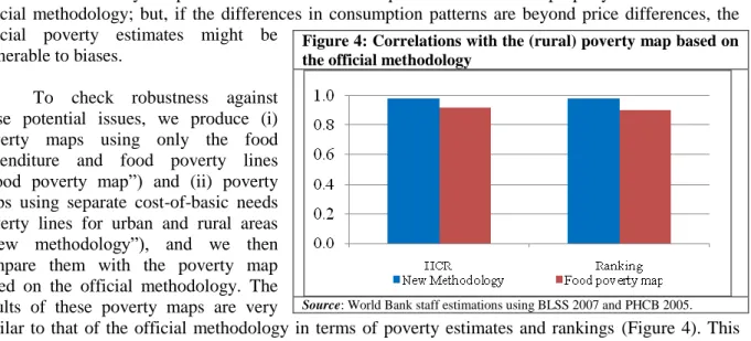
55. There are potential concerns on poverty line estimation and data in that (i) some of non-food expenditure appears too lumpy in some rural areas; (ii) differences in consumption patterns in urban and rural areas can be beyond price differences. Note that price differences are properly addressed in the official methodology; but, if the differences in consumption patterns are beyond price differences, the official poverty estimates might be
vulnerable to biases.
56. To check robustness against these potential issues, we produce (i) poverty maps using only the food expenditure and food poverty lines (“food poverty map”) and (ii) poverty maps using separate cost-of-basic needs poverty lines for urban and rural areas (“new methodology”), and we then compare them with the poverty map based on the official methodology. The results of these poverty maps are very
similar to that of the official methodology in terms of poverty estimates and rankings (Figure 4). This suggests the abovementioned potential data and methodological issues are not substantial.
57. Overall, test results confirm the validity of the poverty map. Formulas predict true consumption expenditure well. The error structures are correctly estimated, though there is still room for improvement in rural areas. Simulations methodology is reliable. These facts lead to accurate final results, including in rural areas. Urban results, on the other hand, are less reliable. Overall, the ELL estimates are consistent with the official poverty estimates. In comparison to other countries, formulas are in general better;
simulations are more reliable; but final results are less accurate, even for rural areas, due to small sizes of population in some areas.
Figure 4: Correlations with the (rural) poverty map based on the official methodology
Source: World Bank staff estimations using BLSS 2007 and PHCB 2005.
16 Section III: Poverty Mapping Results
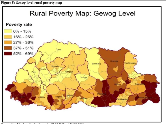
58. The most prominent result from the poverty mapping exercise of Bhutan is the production of a disaggregated poverty headcount rate at the gewog level. The rural poverty map at the gewog level is shown in Figure 5 while the poverty numbers are shown in Annex I, Table A-1.
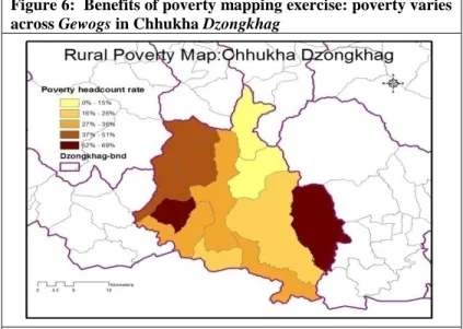
59. Landlocked geography creates many isolated remote areas. National or dzongkhag-level poverty estimates hide rich diversity in living standards across gewogs. For example, Chhukha dzongkhag is an average dzongkhag in terms of well-being, its poverty rate at 20.3 percent while the national poverty rate is at 23 percent. However, its gewogs vary dramatically in terms of poverty headcount rates. Some gewog in Chhukha dzongkhag record among the highest poverty incidences in the country, while some record among the lowest. The use of dzonghag level poverty estimates cannot reflect the large variation in poverty incidence within a dzongkhag. The rural poverty rates range from 6 percent in Bjachho gewog to 55 percent in Logchina gewog . The map in Figure 6 lucidly depicts the variation in poverty.
Figure 5: Gewog level rural poverty map
Source: World Bank staff estimations using BLSS 2007 and PHCB 2005.
17 60. In terms of policy implications,
poverty maps are useful to identify such pockets of poverty and also of wealth. It is useful to fine-tune policies and resource allocation for each small area.
For example, providing the same amount of recourses to rich and poor areas is not efficient. Poverty maps allow us to fine-tune policy interventions based on needs.
Additionally, the disaggregated data of development indicators enhances the
“results-based approach” in the 10th plan.
Poverty Headcount Rate vs. Number of Poor Population
61. The poverty headcount rate refers to the proportion of people who live below the poverty line; it reflects the prevalence of poverty in a specific area. It is the most popular indicator of poverty. In addition, one can also look at the absolute number of the poor population. Poverty maps provide geographical depictions of where the poor are populated (as shown in the upper map of Figure 7) and where the percentage of poor populations is high (as shown in the lower map of Figure 7).
62. Geographic patterns of poverty in Bhutan vary by area. Areas in the southwest around Samtse dzongkhag have high poverty rates with large number of poor people. On the other hand, dzongkhags in the east have high poverty rates but fewer poor people due to lower population density. These geographic patterns of poverty—showing areas have high poverty rates or where the poor are located—
can be used to calibrate poverty alleviation strategies to fit local conditions. A poverty alleviation strategy might need to take into account the geographic patterns of poverty.
Figure 6: Benefits of poverty mapping exercise: poverty varies across Gewogs in Chhukha Dzongkhag
Source: World Bank staff estimations using BLSS 2007 and PHCB 2005.
Figure 7: Poverty Rates and Number of Poor in Rural Areas
Source: World Bank staff estimations using BLSS 2007 and PHCB 2005.
18 Poverty maps with other geo-referenced data
63. Geo-referenced poverty data is useful to locate pockets of severe deprivation, which cannot be identified from poverty estimates at the dzongkhag level. However, locating poor areas is not enough. It is important for policy makers to identify what are bottlenecks or constraints limiting economic opportunities in these areas. For this purpose, it is instructive to overlay the poverty map with other geo- referenced data.
64. Despite its apparent advantages, it is important to note such comparisons can only show visual correlations rather causal relationships. For example, even if poverty and market accessibility are highly correlated, this does not necessarily mean improving market access reduces poverty. There is always a possibility that non-poor areas attract road and other infrastructure investment. To understand a causal relationship, a further careful empirical analysis is necessary.
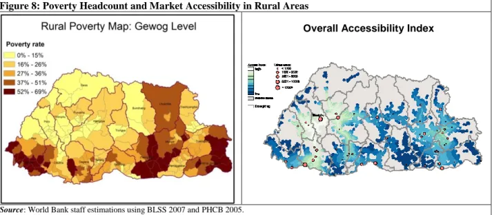
(i) Market Accessiblity and Poverty
65. Market access and connection to road networks are the main drivers of poverty reduction and development in rural areas. The maps in Figure 8 show the relationship between market access and poverty. Access to markets and road network is shown by the Overall Accessibility Indicator, which is measured by the size of markets weighted by travel time, while road network is shown in the bottom map6. Travel time was estimated from the road network information using GIS software. This measure works as follows: even when there are many large markets and cities, if they are very far away from a village, the village’s accessibility indicator takes a low value. On the other hand, even when there is only one medium-size market, if a village is located near the market, the village’s accessibility indicator takes a high value. The accessibility data was plotted only for areas which are populated. Areas with lighter colors have better access to markets. The calculation of market accessibility indicators is explained in detail in Annex III.
66. Looking at the maps, we can see a pattern between rural poverty and market access. Overall, poor areas tend to have low access to markets and poor connection to road networks. For example, one of the poorest dzongkhags, Zhemgang, has very little access to road networks and markets. On the other
6 Overall accessibility is calculated for each place as the sum of the population of all towns in its vicinity, inversely weighted by the travel time to reach them. It is also often called “population potential”.
Figure 8: Poverty Headcount and Market Accessibility in Rural Areas
Source: World Bank staff estimations using BLSS 2007 and PHCB 2005.
Overall Accessibility Index
19
hand, areas in western Bhutan are highly connected to markets and also have the lowest poverty levels.
However, it is worth noting that there are some exceptions in the north (Gasa dzongkhag), where poverty incidence is low but the market access is also limited.
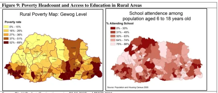
Access to Education and Poverty
67. Education is universally agreed to be a factor that can help people out of poverty, by giving them better jobs and higher earnings. Access to education, regardless of children’s circumstances and their parent’s income, improves economic opportunities for the next generation of Bhutanese, and facilitates growth and poverty reduction for the country as a whole.
68. Bhutan has made tremendous progress in access to education in rural areas; however, several challenges remain. Access to education is shown in the map by the percentage of population aged 6 to 18 years old who are attending school (Figure 9). The map shows that there are many areas where few children attend school, and many of these gewogs tend to also have high poverty rates.
Figure 9: Poverty Headcount and Access to Education in Rural Areas
Source: World Bank staff estimations using BLSS 2007 and PHCB 2005.
69. Rural electrification is often regarded as a vehicle for rural development, and helps to improve the quality of basic services like education and health. Bringing electricity to the rural population not only improves their quality of life, but also promotes economic activity and increases agricultural production.
70. Rural electrification in Bhutan varies dramatically across the country, ranging from almost full coverage to none. The map on the right shows the percentage of households with an electricity connection in rural areas. The areas with high electrification rates tend to be concentrated in rich and densely populated gewog in Paro, Chhukha, Thimphu, and Phunaka. On theother hand, rural eletrification is relatively low in the rest of the country (Figure 10).
20
Figure 10: Poverty Headcount and Access to Electricity in Rural Areas
Source: World Bank staff estimations using BLSS 2007 and PHCB 2005.
(iv) Gender and Poverty
71. The linkage between gender and development has gained much attention among development practitioners. Women’s engagement in economic activities can bring more income and other resources to households and elevate their living standard. One of the most prominent indicators in women’s economic engagement is the female labor force participation, which represents all economic engagements, both paid and unpaid.
72. The spatial relationship between location of poverty and female labor force participation is shown in Figure 11. Overall, there is no clear spatial pattern between rural poverty and female labor force participation. Such results call for additional studies on the relationship between gender and poverty. Gender is generally a complex issue, involving multiple layers of socio-economic variables as well as local culture and traditional practices. Incorporating such factors into the analysis can shed more light onto the gender and development connection in the case of Bhutan.
Figure 11: Poverty and female labor force participation in rural areas
Source: World Bank staff estimations using BLSS 2007 and PHCB 2005.