NEPAL
Small Area Estimation of Poverty, 2011 Vol: I
April 2013
Government of Nepal
National Planning Commission Secretariat Central Bureau of Statistics
Public Disclosure AuthorizedPublic Disclosure AuthorizedPublic Disclosure AuthorizedPublic Disclosure Authorized
78812
Executive Summary
Nepal Small Area Estimation of Poverty1
Small area estimates of poverty have become useful tool in targeting poverty reduction by geographic areas. By now, more than 60 countries have small area estimates of poverty (“poverty maps”). For Nepal, this is the second poverty map produced after a gap of seven years in collaboration with the Central Bureau of Statistics, Nepal. Visualized on geographical map, small area estimates can convey to audiences of all literacy levels the scale and distribution of poverty not possible by tabular data. Further, poverty maps can be super-imposed on spatial variables such as climate or infrastructure to analyze spatial determinants of poverty.
Small area estimates improve the accuracy and disaggregate spatially the poverty estimates made from survey data. The Nepal Living Standards Survey is representative at the level of 14 broad strata, but district development committees in particular value information at a lower level such as the VDC – some 3970 of them. While the (NLSS) 3 includes too few observations to produce estimates at district level or lower.
The small area estimates in this report are based mainly on most recent information from Nepal Living Standards Survey 2010-11 and Nepal Census 2011. Auxiliary data sources include VDC- level GIS information obtained from the Vulnerability Analysis and Mapping unit of World Food Program Nepal. Variables are: mean elevation in kilometers, mean slope in percentage, height range, standard deviation of height, population density in inhabitants per square kilometer, distance to the district headquarters, length of road in kilometers (by ilaka), length of road in kilometers per thousand inhabitants (by ilaka), length of rivers in kilometers. An improved accessibility measure called "Kosh" (measures how many hours it takes for a normal person to walk from the VDC to the district headquarters) available with the Election Commission was also used to enrich the estimates.
Besides using more recent data and improvements in methodology, the small area estimates in this report remedy an important limitation of the poverty map of 2006i by providing estimates as close as the VDC/Municipality level. Though the previous poverty map provided estimates for
1This is a product of collaborative work between the World Bank and the Central Bureau of Statistics, Nepal. From the World Bank, Peter Lanjouw, Marleen Marra, Prem Sangrula and Srinivasan Thirumalai (Task Team Leader) worked with a team of CBS staff drawn from the Household Surveys, Population, GIS and Prices sections led by the Director General U. Malla. The core team of CBS staff were: Binod Sharan Acharya, Gyanendra Bajracharya, Dinesh Bhattarai, Bed Prasad Dhakal, Devendra Karanjit, Shyam Prasad Neupane and Jayakumar Sharma. GIS help for creation of new shapes and visualization was ably provided by Brian Blankespoor (DECCT). Chris Gerrard (DECDG) and Minh Cong Nguyen (SARCE) helped immensely with Tableau customization for developing the online tool. The team would like to thank peer reviewers Professor Chris Elbers, Professor Pushkar Bajracharya, Mr. T. Bastola and Maria Eugenia Genoni.
967 ilakas, for development planning proposes, estimates at even finer geographic levels would have been more useful. This exercise of small area estimation of poverty provides statistically reliable poverty measures for 2344 VDCs or groups of VDCs of Nepal. When statistical reliability is doubtful to estimate VDC level poverty, similar VDCs have been combined to generate reliable poverty estimates for the select aggregate of similar VDCs inside a given ilaka.
For all the VDCs, even for those precise estimates cannot be made, confidence bands for poverty estimates are provided..
This report presents 2010/11 small-area estimates and maps for Nepal at the 75 district, 967 ilaka and 2344 "target area" level, of poverty incidence, poverty gap, and poverty severity. The report also provides maps of the number of poor and their average consumption.
The findings confirm the spatial distribution of poverty in Nepal. Poverty - both as a rate and headcount - is high in the hilly areas of Far West and parts of Mid-West. The percentage of poor varies from negligible in parts of Kathmandu to 75 percent in parts of Gorkha district. A comparison with the poverty map of 2006 shows that though prosperity is spreading in Nepal, it has a hard time moving West and climbing Hills. Poverty concentration in the East and Central has declined while it increased in the rest. Nearly half the small areas have poverty higher than the national average of 25.2 percent and contain two-thirds of the poor in Nepal.
The character of the spatial distribution of poverty in Nepal is not new but the estimates at 2344 small areas along with their standard errors should help in better design of development interventions. While it is straight forward to target development activities in areas with extreme poverty, in areas where poverty is not distinctly different, randomized experiment designs can be used to pick appropriate interventions that are most effective.
The poverty maps could usefully be expanded to other indicators of welfare such as nutrition and food security like in 2006. Detailed spatial distribution of poverty offers an opportunity to explore further the causes of poverty trends in Nepal. When combined with the spatial distribution of correlates of poverty such as access to roads, schools and health facilities, and other variable of economic geography, one can further our understanding of the persistence of pockets of poverty in Nepal.
Table of Contents
1. Introduction ... 1
2. Methodology ... 2
2.1 Small-area estimation ELL method ... 2
2.2 A note of caution ... 4
3. Data sources and description ... 5
3.1 NLSS3 and 2010/11 Population Census ... 5
3.2 Common and comparable variables ... 6
3.3 Definition of "target area" ... 7
4. Results ... 9
4.1 Strata-level results in comparison with NLSS3 ... 9
Table 2: Predicted poverty rates on the target level - by stratum and in comparison to NLSS3 poverty rates ... 10
4.2. District, ilaka, and target-level results ... 11
Table 3: Summary statistics of predicted poverty rates ... 12
4.3 Maps ... 12
5. How reliable are these maps?... 14
5.1 tests for over-fitting ... 14
Table 4: Over-fitting test comparing observed and predicted FGT(0) in a subsample of the NLSS3 survey ... 15
5.2 Breakdown of standard errors ... 15
6. Conclusions and suggestions for follow-up work ... 17
References ... 19 Appendix I: Further information on data and selected models and poverty maps ... Error! Bookmark not defined.
... Error! Bookmark not defined.
Appendix II: Tables with small area estimations of poverty on the level of the district, ilaka, target-level, and VDC. Error! Bookmark not
defined.
Figures
Figure 1- Belts and district boundaries of Nepal ... 8
Figure 2 - Poverty incidence on target-area level ... 12
Figure 3 - Poverty gap on target-area level ... 13
Figure 4 - Poverty severity on target-area level... 13
Figure 5- Number of poor (FGT(0)) on target-area level ... 14
Figure 6 - Standard error of FGT(0) by target area size (number of households) ... 16
1
1. Introduction
Knowledge of living standards at the level of towns, cities, districts, or other sub-national localities can help to inform decision making on a variety of issues. Notably, poverty reduction efforts can benefit from information on welfare outcomes at the level of the most disaggregated administrative jurisdictions. Poverty indicators, such as the headcount rate, estimated at the national or urban/rural level, are unable to capture important differences between small areas such as districts, Village Development Committees (VDC) or municipalities. In the case of Nepal, the nationally representative Nepal Living Standards Survey is representative at the level of 14 broad strata, but district development committees in particular value information at a lower level such as the VDC. While the (NLSS) 3 includes too few observations to produce estimates at district level or lower, there does exist a Population Census for Nepal, covering the entire Nepali population. Unfortunately, the Census does not collect the detailed expenditure information needed to estimate reliable and readily interpretable poverty measures.
Small-area estimation is a statistical technique that improves accuracy of direct survey estimates of welfare for small areas by combining survey data with other sources such as the population census (see for instance Ghosh and Rao, 1994, Rao, 2003). This method has been adapted to the generation of small-area estimations of poverty by Elbers, Lanjouw and Lanjouw (2002, 2003, - henceforth ELL). The ELL method combines household survey data and census data at the unit record level, making it possible to estimate reliable poverty indicators at local level. To date this method has been applied in more than 60 countries with as objective informing policy-makers of the spatial pattern of poverty and other welfare indicators in their respective countries (see Bedi et al., 2007 for a review of applications). In 2006, Nepal's Central Bureau of Statistics, The World Food Program, and The World Bank, worked together to produce a poverty map for Nepal using the 2003/04 NLSS, the 2001 Nepal Demographic and Health Survey and the 2001 Population Census (CBS et al, 2006). The present report updates the 2006 results for Nepal in three ways. First, it uses the recently published 2010/11 round of the NLSS and 2011 Population Census in order to produce an updated description of the spatial patterns of poverty. Second, it incorporates new methodological refinements aimed at improving modeling of the standard error (as detailed in the methodology section below). Third, in an effort to improve practical usability of the results, estimates are produced at the sub-ilaka or VDC level - where possible - instead of sticking with the ilaka level that was used in 2006.
By combining small-area estimates with GIS information, the resulting "poverty maps" can be used to highlight detailed geographical variations with high resolution. Maps can be powerful tools for convening complex messages in a visual format for both technical and non-technical
2
users.0F2 This report presents 2010/11 small-area estimates and maps for Nepal at the district, ilaka and "target area" level, of poverty incidence, poverty gap, and poverty severity (interchangeably referred to as FGT (0), FGT (1) and FGT (2) as per standard notation referring to Foster, Greer, and Thorbecke; 1984). The report also provides maps of the number of poor and their average consumption. As the newly introduced target areas are generally smaller than conventional aggregation levels, special attention is devoted to investigating the precision of the point estimates and to interpretation of the results.
2. Methodology 2.1 Small-area estimation ELL method
To exploit the detailed expenditure information of the NLSS3 household survey and the entire population coverage in the Census, we apply the small area estimation method developed by Elbers, Lanjouw and Lanjouw (Henceforth, ELL; 2002, 2003). The exercise involves three broad steps. First, it requires selecting a set of variables that are common to the household survey and the Population Census. Common variables include household characteristics of education, housing quality, durables, ethnicity, etc. Besides being common, it must be established that these variables are statistically indistinguishable and similarly framed. Surprisingly, many common variables between the NLSS III survey and the 2011 Population Census have been found to have different means, which will be discussed in more detail in chapter 3. In addition, GIS information at the VDC level and household variables' area means are calculated from the census and merged with the survey. Adding area means, calculated the target level at which poverty is to be estimated, or below, helps to explain location effects and has been shown to improve estimates markedly (Elbers et al., 2002).
Second, observed expenditure in the survey is regressed on selected common variables as follows:
( ) , (1)
where ln(ych) is log of per capita expenditure of household h in cluster c, Xch the vector of selected explanatory variables, the vector of regression coefficients, and is the vector of disturbances. The subscript ch refers to household h living in cluster c, the VDC in this case. For the analysis in this report, this expenditure modeling (or, “beta model”) is done for three regions separately: Central & Eastern regions, Western region, and Midwestern & Farwestern regions.
We thus allow for variation in the relationship between expenditure and the selected variables
2 "Poverty mapping" can be extended to allow for deeper understanding of correlates of poverty at the disaggregated level. For example; maps can display poverty incidence together with non-farm employment, or incidence of disease or school enrollment or level of education and so on. Spatial representation of school locations, infrastructure, health posts etc., can therefore complement regression analysis to help us understand the influence of these covariates and their interaction with poverty..
3
among these three broad areas. As the level of aggregation at the target level is particularly low, this course of action helps to reduce standard errors on poverty estimates and thus to improve precision. In addition, estimating three separate models also helps to confront this above- mentioned concern with non-comparable variables, across the survey and census. This is because at the region level, comparability across the two data sources is better. Estimating separate models thus provides more space to include meaningful covariates of expenditure into (1).1F3 Consumption models include variables that are selected on the basis of being common and comparable, and being meaningful and statistically significant at least the 5% level.
Estimation of (1) by simple OLS gives estimated residuals ̂ (that are estimates of overall residuals ). These residuals are broken down into two components: a cluster specific random effect and an uncorrelated household error term:
̂ ̂ (2)
where ̂ is the cluster-specific random effect, calculated by simply taking within-cluster means of the total estimated residual, and is the resulting household-specific random effect. It is worth noting one critique of the ELL methodology that argues that the level of precision of the results could be overstated if the error structure is misspecified. In particular, if standard errors are correlated at a level higher than the cluster, but autocorrelation is modeled at the cluster level, then calculated standard errors could be smaller than justified (Banerjee et al., 2006; Tarozzi and Deaton, 2008). However, the ELL method doesn’t insist on modeling autocorrelation at the cluster level, (Elbers et al., 2008), and that careful incorporation of area-level means can help to ensure that the location effect is small. A recent paper using Brazilian census data to validate the ELL method, finds that associated standard errors can be both realistic and sufficiently narrow to yield usable estimates. (Elbers et al, 2008). In general, the better model (1) is at capturing location effects, the smaller the potential for underestimating standard errors. In this paper we model the location effect at the cluster level which is (mostly) below the level at which the poverty rates are estimated. However, we apply the location effect at the target level in our simulations.2F4 We basically assume that the observed correlation of the deviation in predicted expenditure at the level of the VDC applies in its entirety across all households at the higher level (target area, ilaka, or district). As argued by Elbers et al (2008), this is a quite conservative approach as, in all likelihood, only a fraction of the correlation between households in the VDC applies to this higher level. As a result we can thus be fairly confident that the standard errors in this paper are not overstating the precision of our estimates.
To allow for heteroskedasticity in the household error component, a model of the variance of conditional on selected variables can be applied. Such a model (“alpha model”) is used for the
3 We also fitted one national model to the data for comparison, and find that the point estimates of poverty incidence are highly correlated (correlation of about 0.9) . However, the results of the national model are somewhat less precise.
4 We say “mostly” as some VDC’s are equal to the “target level” if they are large enough.
4
Central/Eastern and Western regions but not for the Mid/Farwestern region.3F5 Tables A5-A9 in Appendix I present the three beta models and the two alpha models.
Third, expenditure of a household in the Census is predicted as follows:
̂ ( ) ̂ ̂ ̂ (3)
where ˆ,
ˆc and
ˆch denote the estimates for ,
c and
ch. Point estimates as well as standard errors of the welfare indicators are calculated by Monte-Carlo simulations. In each simulation, a set of values ˆ and
ˆch are drawn from their estimated distributions, and an estimate of expenditure and the poverty rates are obtained.Originally, the ELL method also draws location errors c from their estimated unconditional distributions. For those target population for which sampled data happen to be available, this approach does not make optimal use of available information. An approach proposed by Molina and Rao (2010) combines the simulation-based approach with what is referred to as Empirical Best, which uses the observed distribution of location error in the sampled data. With the adjustment that the distribution functions of the errors are estimated non-parametrically, this approach has been implemented in the PovMap software. The estimations in this report use the Empirical Best option – thus drawing errors from their estimated distributions for all areas that are not represented in the NLSS3 while drawing from their observed distributions for those that are sampled.
For all three regional models, and in each simulation, ̂ ( ) is trimmed at the observed minimum and maximum values in the Survey. Subsequently, the average point estimate and standard deviation of 500 simulations of (3) is calculated. Finally, predicted expenditure and poverty for all households in the Census is aggregated to generate VDC-, target area-, ilaka-, and district-level estimates. For the calculation of poverty indices we apply a poverty line of 19,261 Nepali Rupees per person/year.
2.2 A note of caution
While the practice of estimating the consumption model (1) on three separate regions, instead of estimating one model for the whole of Nepal, creates the benefit of potentially capturing the relationship between expenditure and the observables more closely it also makes the results more prone to over-fitting. In general, adding more explanatory variables and reducing the number of
5 Alpha models can reduce the influence of large residuals, thereby potentially improving small-area results.
Typically their explanatory power is low, as we also find for our alpha models; Central/Eastern R2=0.023, Western R2=0.035. For Mid/Farwestern, adding the alpha model causes point estimates to change only marginally while reducing average precision.
5
observations in the consumption model will likely improve the apparent fit of the model measured by R2. However, the larger the number of explanatory variables relative to the number of observations in the sample, the larger the uncertainty associated with them. It is therefore important to carefully examine the fit of the models. This is done by taking a 50% random subsample of each survey region; treating one half ("subsample 1") as the household survey and the other half ("subsample 2") as the census. Using these datasets while repeating steps 2 and 3 outlined above, we can then compare the predicted poverty incidence in subsample 2 against the actual poverty incidence that is observed. Since the households in subsample 2 are not included in the sample on which the model is calibrated, being able to predict poverty accurately suggest that the consumption model is not too specific. A second way in which we ascertained that the consumption model is general enough that our final consumption models include only variables that are statistically significant at the 5% level on this random 50% subsample of the regions.
Another thing to keep in mind is the usability-certainty trade-off. Introducing a lower level of aggregation than that has been used before makes these maps and estimates more attractive to use for anti-poverty policy-making in Nepal. However, this comes at the cost of precision in the estimates. The fewer the households in the area, the higher the standard error typically is, and the less precise the point estimates. Especially when ranking target areas in terms of poverty rates, the user is strongly advised to take the reported standard error into account.
3. Data sources and description 3.1 NLSS3 and 2010/11 Population Census
The Nepal Living Standards Survey 2010/11 (henceforth - NLSS3) is the third round of its kind conducted in Nepal (the first having been fielded in 1995/96) and follows the general structure of the World Bank's Living Standard Measurement Study (LSMS) surveys. It is an integrated survey covering a wide range of topics ranging from consumption expenditure to agricultural production, education and remittances. It is based on the 2000 Population Census sample frame.
In the first sampling stage, 800 Primary Sampling Units that are identical to those in the 2007/08 National Labor Force Survey are selected. They fall into six strata.4F6 In the second-stage, 500 of these PSU's were selected with an explicit sub-stratification that culminates in the 14 strata of the NLSS3.5F7 This selection was done proportional to size - using the number of households as a measure of size. Finally, 12 households per PSU were selected randomly6F8. Sampling weights have been calculated as the inverse of the primary sampling unit's probability of being selected.
Note that the probability of being selected, and thus the sampling weight, is based on the sample
6 These 5 strata are: Mountains; Urban Kathmandu, Other urban in hills, Other urban in terai, Rural hills, Rural terai
7 These 14 strata are: Mountains, Urban Kathmandu, Other urban in hills, Rural eastern hills, Rural central hills, Rural western hills, Rural midwestern hills, Rural farwestern hills, Urban terai, Rural east terai, Rural central terai, Rural western terai, Rural midwestern terai, Rural farwestern terai.
8 For more details on sample design see NLSS III Statistical Report, volume 1, Central Bureau of Statistics.
6
frame of the 2000 Population Census as well as forecasts of the population size in 2010/11.
NLSS3 finally includes 5,988 households and 28,474 individuals.
The second data source used to produce small-area estimates of welfare is the Nepal Population Census 2010/11. The National Planning Commission and Central Bureau of Statistics were very supportive to provide census data at unit level for all common variables with the NLSS3. The number of non-institutional households is 5,423,297. After dropping those that had a missing level of education of the household head, we end up with a dataset of 5,337,972 households.
Auxiliary data sources include VDC-level GIS information obtained from the Vulnerability Analysis and Mapping unit of World Food Program Nepal. Variables are: mean elevation in kilometers, mean slope in percentage, height range, standard deviation of height, population density in inhabitants per square kilometer, distance to the district headquarters, length of road in kilometers (by ilaka), length of road in kilometers per thousand inhabitants (by ilaka), length of rivers in kilometers (a more detailed description can be found in CBS et al, 2006). This information dates back to 2006, but since most variables don't change (rapidly) over time they are still useful for the analysis in this report. However, as we expect that accessibility is a particularly important indicator for welfare, we added another variable called "Kosh". The CBS prepared this variable at the VDC level, and it measures how many hours it takes for a normal person to walk from the VDC to the district headquarters.
3.2 Common and comparable variables
Table A1 in Appendix I presents the mean, minimum, maximum, and standard deviation of common variables between the survey and the census. As the census enumeration was done in June 2011 closely on the heels of the survey (February 2010 to February 2011), one would expect very little variation between both data sources. Yet, we find that for a number of household-level variables the census mean does not lie within two standard errors of the survey, i.e. they are statistically different. One potential explanation for this is that the Census is conducted four months after the Survey, a time lapse of 10 months from the mid-point of theone year survey period and the census date. If over the span of that short period the Nepali population has become better off in terms of some major indicators, such as the construction material of their homes or the level of education of the household head, then this could be a reasonable explanation. Alternatively, the difference could be attributed to misrepresentation of the population in the NLSS3 household survey. Population weights convert the survey sample to strata-level and nationally representative numbers, but they are based on a forecast of the 2010 population made in 2001. However, even after adjusting the weights based on the actual 2011 Census population, the survey and census means of the majority of the common variables still don't line up. Alongside these household-level variables, Census means on the level of the ward and the VDC are calculated and added to the common and comparable variable pool from which
7
to select the models. Even those variables that are incomparable on the household level are comparable at higher levels, such as VDC, and could thus be added.
As comparability of the survey and census variables is a strong requirement for the small-area estimation methodology to provide accurate results, this issue poses a challenge7F9. For the analysis in this report, we take the conservative approach to limit the set of candidate variables to those that are strictly comparable between survey and census in the regions we are working with.
Tables A2-A4 in Appendix I present the statistics for the variables that were selected into the three regional consumption models.
3.3 Definition of "target area"
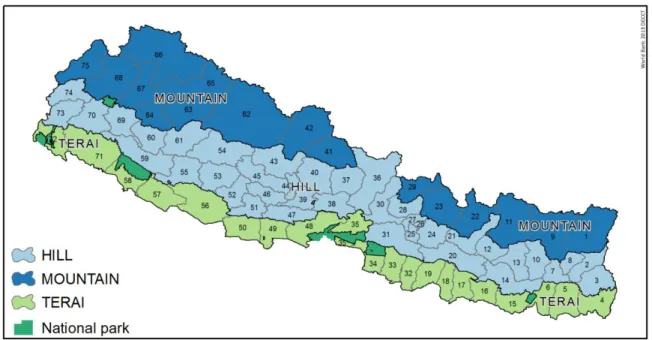
Besides the five regions that are already introduced (East, Central, Midwest, West and Farwest), Nepal is divided into three ecological zones that run from east to west and that are defined by their altitude; Mountains, Hills, and Terai. Terai areas, or plains, are below 610 meters above sea level. They are generally the most fertile and run alongside the southern border. The Hills are between 610 and 4,887 meters high, and include also Kathmandu and the touristic hotspot of Pokhara. Mountains are most sparsely populated and include all areas above 4,887 meters;
obviously with much harder living conditions and lower levels of infrastructure. The country is divided into 75 districts that range in population between 5,819 (Manang) and 1,688,131 (Kathmandu). The map in Figure 1 shows the district boundaries and the three ecological belts in the country.
9. It is beyond the scope of this report to attempt to discover the cause of the disagreement between variables in the household survey and population census. But clearly this is an issue of concern.
8
Figure 1- Belts and district boundaries of Nepal
Each district is divided into between 9 and 20 ilakas, which are collections of VDC's and municipalities which are respectively represented in the district development committee. Ilaka's are officially recognized by the Ministry of Local Development. The 2006 poverty maps are produced at the Ilaka level.8F10
As indicated before, the Central Bureau of Statistics is with technical support from the World Bank, making an effort to produce small-area estimates at an as detailed as possible level of geographic disaggregations. The main reason for this is to improve usability of the maps and poverty estimates, for instance by district development committees that want to allocate social assistance. What resulted is what we call "target area". For mountain areas, which are sparsely populated, this target area is equivalent to the ilaka. None of the mountain areas have sub-ilaka target areas. For all VDC's in hills and terai, a more hands-on approach is adopted. First, if a VDC is sufficiently large and thus a precise estimate of poverty can be produced, the target area is equivalent to just that one VDC. This approach is adopted for all municipalities, for instance.
Second, other VDC's are combined on the basis of three criteria: 1) VDC's are adjacent, 2) VDC's are similar in term of characteristics, and 3) the resulting target areas are reasonably large.9F11 The distribution of the resulting target areas, as well as that of districts, ilaka's, and
10 However, they redifined the original ilaka's to be the rural part of existing ilaka's only (927), and added each of the 58 urban municipalities as a new ilaka, resulting in a total of 976 new ilaka's. For the ease of comparison, we adopt the same definition of ilaka in this report.
11 Similarity is judged by a crude estimate of FGT(0), as that is the "best guess" of the VDC's level of welfare given the variable matrix this prediction is based on. It thus incorporates information on education levels, quality of the house, ownership of durables, GIS information such as average altitude and mean slope of the VDC, district characteristics, etc. "Reasonably large" replaced the original goal of aiming for target areas of at least 5,000 households when this often proved to be contrast with the other criteria and with CBS' aim to produce estimates for disaggregated sub-ilaka areas.
9
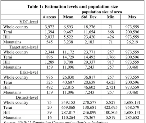
VDC's, is outlined in Table 1. As per the way target areas are defined, the table shows that in mountain areas, their size is equal to those of ilaka's and that in hill and terai areas their average size lies between that of ilaka and VDC. Table A15 in the Appendix can be used as a reference to look up which VDC’s fall into which target area
Table 1: Estimation levels and population size population size of area
# areas Mean Std. Dev. Min Max
VDC-level
Whole country 3,972 6,593 18,276 71 973,559
Terai 1,394 9,467 11,654 868 200,596
Hill 2,033 5,522 23,420 426 973,559
Mountains 545 3,238 2,183 71 26,219
Target area-level
Whole country 2,344 11,172 23,771 257 973,559
Terai 896 14,729 14,492 1,766 200,596
Hill 1,289 8,708 29,337 917 973,559
Mountains 159 11,096 7,243 257 30,460
Ilaka-level
Whole country 976 26,830 36,817 257 973,559
Terai 325 40,607 20,639 4,623 200,596
Hill 492 22,815 46,602 2,721 973,559
Mountains 159 11,096 7,243 257 30,460
District-level
Whole country 75 349,153 278,577 5,827 1,688,131
Terai 20 659,868 138,681 422,695 958,579
Hill 39 287,817 246,099 100,805 1,688,131
Mountains 16 110,264 75,367 5,819 285,652
Source: 2010/11 Population Census and author’s calculations.
4. Results
4.1 Strata-level results in comparison with NLSS3
To get a general idea of the larger welfare trends, as well as to judge the accuracy of our prediction models, we first compare the small-area estimations against the poverty incidence directly observed from NLSS3 at the strata level. This is the lowest level at which the household survey is representative. Strata-level poverty rates are presented in Table 2. The Z-value can be used to assess whether the predicted measure of poverty incidence FGT(0) is within two standard errors from the observed FGT(0) in the NLSS3.10F12 These Z-scores indicate that the small-area estimations of poverty incidence based on our regional models are generally within two standard errors of the poverty incidence rates in the survey. However, two out of the 15 results fall outside the confidence interval of two standard errors. Poverty incidence in rural central hill and rural western hill are predicted to be respectively 17.4% and 20.2% compared to direct estimates from the survey of respectively 29.4% and 28%. Another thing to be noted from the table is that the three regional models seem to do similarly well in predicting poverty. Poverty for Nepal as a
12 It is defined as: Z = ( FGT(0) census - FGT(0) survey ) / √[ (S.E. census)2 + (S.E. census)2]. The value of Z should thus not exceed │2│for both measures to represent the same poverty incidence.
10
whole lies well within the 2 standard error bounds. It also reflects the trend of a poverty rate that is decreasing over time: the country's headcount rate continues its steady decline from 60 % in 1995/96, to 49 % in 2003/04, to 25% in 2010/11, using comparable concepts of consumption (monthly recall) and poverty lines.
The small area estimations of poverty, though generally within the confidence interval, are for the majority of strata somewhat lower than the direct estimates from the household survey. This could be related to an issue noted earlier - census means of common variables being mostly 'better off' than population-weighted survey means.
0BTable 2: Predicted poverty rates on the target level - by stratum and in comparison to NLSS3 poverty rates
Observed poverty rates NLSS3 Predicted poverty rates at the target level Z- value
# households
holds
FGT(0) # households holds
FGT(0) FGT(1) FGT(2)
100/Mountain Mean 408 0.423 363,698 0.398 0.104 0.039 -0.552
S.E. mean 0.043 0.014 0.005 0.002
218/Urban-Kathmandu Mean 864 0.115 273,733 0.110 0.022 0.007 -0.307
S.E. mean 0.015 0.005 0.002 0.001
219/Urban-Hill Mean 480 0.087 335,015 0.104 0.023 0.008 0.613
S.E. mean 0.021 0.019 0.005 0.002
221/Rural-Hill-Eastern Mean 384 0.159 318,511 0.186 0.037 0.011 0.860
S.E. mean 0.030 0.008 0.002 0.001
222/Rural-Hill-Central Mean 480 0.294 598,323 0.174 0.040 0.013 -2.279
S.E. mean 0.052 0.009 0.003 0.001
223/Rural-Hill-Western Mean 480 0.280 542,632 0.202 0.047 0.016 -2.125
S.E. mean 0.036 0.006 0.002 0.001
224/Rural-Hill-Midwestern Mean 336 0.316 315,318 0.315 0.074 0.025 -0.034
S.E. mean 0.044 0.007 0.002 0.001
225/Rural-Hill-Farwestern Mean 180 0.476 147,832 0.472 0.128 0.048 -0.052
S.E. mean 0.063 0.008 0.003 0.001
310/Urban-Terai Mean 672 0.220 424,461 0.162 0.039 0.014 -1.442
S.E. mean 0.035 0.020 0.006 0.002
321/Rural-Terai-Eastern Mean 480 0.210 647,025 0.225 0.050 0.016 0.461
S.E. mean 0.032 0.009 0.003 0.001
322/Rural-Terai-Central Mean 480 0.231 713,183 0.242 0.055 0.018 0.390
S.E. mean 0.027 0.006 0.002 0.001
323/Rural-Terai-Western Mean 348 0.223 331,598 0.236 0.056 0.020 0.256
S.E. mean 0.051 0.012 0.003 0.001
324/Rural-Terai-Midwestern Mean 240 0.256 240,088 0.278 0.067 0.023 0.383
S.E. mean 0.056 0.012 0.004 0.002
325/Rural-Terai-Farwestern Mean 156 0.384 171,203 0.351 0.088 0.032 -0.505
S.E. mean 0.065 0.012 0.004 0.002
Total Nepal Mean 5,988 0.252 5,422,620 0.235 0.055 0.019 -1.429
S.E. mean 0.011 0.003 0.001 0.000
Note: the standard error of the observed poverty incidence in NLSS3 is calculated while taking into account population weights as well as the survey's stratified design. Z-value = ( FGT(0) census - FGT(0) survey ) / √[ (S.E. census)2 + (S.E.
census)2]. The value of Z should thus not exceed │2│for both measures to represent the same poverty incidence. Source:
2010/11 NLSS3 and author’s calculations.
11
4.2. District, ilaka, and target-level results
Table A11 in Appendix II presents small area estimations of poverty on the level of the district.
The eight least poor districts are Kaski, Ilam, Lalitpur, Kathmandu, Chitawan, Jhapa, Panchthar and Syangja. Their headcount rates range between 4% and 11.8%. On the other end of the distribution are districts Darchula, Humla, Bajhang, Kalikot and Bajura with headcount rates of more than 50%. It must be stressed that comparisons of poverty across areas should take note of the accompanying standard errors on the point estimates. For instance, although district Jumla has an estimated headcount rate of 49% and district Humla has a headcount rate of 56%; both estimates are associated with high standard errors. In fact, Humla's point estimate of 56% falls within 1.96 standard errors of Jumla's point estimate; meaning that they are statistically indistinguishable at a 95% confidence level. The smaller the size of the target area; the more uncertainty is associated with the predicted poverty rates. The next chapter elaborates further on the interpretation of the results and their precision.
With the previous poverty mapping exercise in 2006, poverty incidence at the ilaka level had been estimated to range between 1% and 82% using the 2001 Population Census (CBS et al., 2006). The current 2010/11 estimations are of similar magnitude, albeit slightly lower in line with steady poverty reduction over the past decade. We find poverty incidence levels ranging between 0.5% and 72.8% on the ilaka level, with an unweighted mean/median of 26.9%/25.7%
(see table A12 in Appendix II). Previous ilaka-level FGT(0) estimates had an average standard error of 0.038, compared to 0.056 now. The 2006 results are likely somewhat more precise as they were able to select a consumption model from a much larger set of common variables;
besides the incomparability issue discusses above, the previous exercise had access to a larger set of data. Particularly, agricultural information on the ownership of livestock, poultry, agricultural land, and ownership of a business was available then, and this information would arguably be a resourceful addition to the models underlying our results. In addition, as discussed above, the strategy for calculating standard errors taken in this study can be regarded as ‘conservative’ and may also account for slightly wider standard errors than the previous poverty mapping exercise.
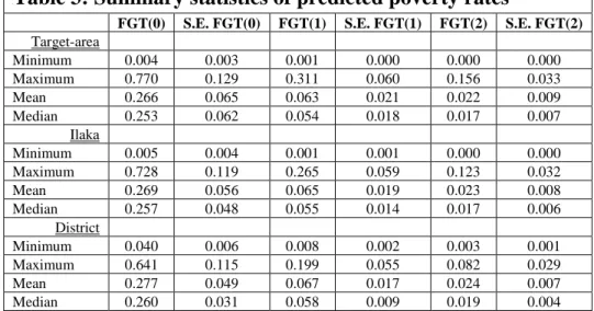
Poverty incidence on the level of target-area ranges between 0.04% and 77%, with an unweighted mean/median of 26.6%/25.3% (see Table A13 in Appendix II, and Table A15 for a reference of which VDC’s fall into which target-area). The standard error is not much larger than that of ilaka's; on average it is 0.065. Table 3 shows for districts, ilaka's and target areas the summary statistics of small-area estimations of their poverty incidence / FGT(0), poverty gap / FGT(1), and poverty severity / FGT(2). The small-area estimation of the headcount rate, poverty gap, and poverty severity are presented in the appendix on the level of the district, ilaka, target- area, and VDC. To underline the uncertainty of the VDC-level estimates, due to their small size, these results are presented in Table A14 in Appendix II by their 95% confidence interval11F13 rather than their point estimate and standard error.
13 calculated by the standard formula: mean ± 1.96 times the standard error.
12
1BTable 3: Summary statistics of predicted poverty rates
FGT(0) S.E. FGT(0) FGT(1) S.E. FGT(1) FGT(2) S.E. FGT(2) Target-area
Minimum 0.004 0.003 0.001 0.000 0.000 0.000
Maximum 0.770 0.129 0.311 0.060 0.156 0.033
Mean 0.266 0.065 0.063 0.021 0.022 0.009
Median 0.253 0.062 0.054 0.018 0.017 0.007
Ilaka
Minimum 0.005 0.004 0.001 0.001 0.000 0.000
Maximum 0.728 0.119 0.265 0.059 0.123 0.032
Mean 0.269 0.056 0.065 0.019 0.023 0.008
Median 0.257 0.048 0.055 0.014 0.017 0.006
District
Minimum 0.040 0.006 0.008 0.002 0.003 0.001
Maximum 0.641 0.115 0.199 0.055 0.082 0.029
Mean 0.277 0.049 0.067 0.017 0.024 0.007
Median 0.260 0.031 0.058 0.009 0.019 0.004
Note: Statistics are not weighted by size of the area and the mean and median should thus be interpreted as pertaining to an average and median area (not an average / median person in the country). Source: author’s calculations.
4.3 Maps
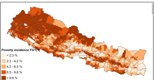
Maps of the average consumption level, poverty incidence, poverty gap, and poverty severity, and the number of poor on the target-area level are presented below in Figures 2-5. Maps on the level of VDC, District and Ilaka can be found in Appendix I; Figures 7-21.
Figure 2 - Poverty incidence on target-area level
13
Figure 3 - Poverty gap on target-area level
Figure 4 - Poverty severity on target-area level
14
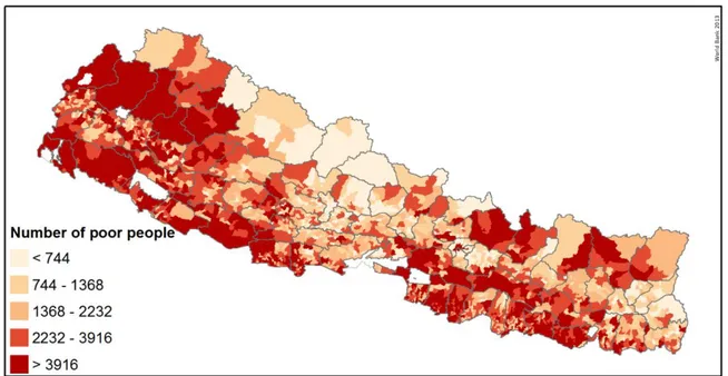
Figure 5- Number of poor (FGT(0)) on target-area level
5. How reliable are these maps?
5.1 tests for over-fitting
To ascertain that the coefficients estimated with the beta and alpha models capture the general relationships between expenditure and observables, rather than being only relevant for a limited set of survey households, all regions are subject to over-fitting tests. They are carried out in accordance with their description in the methodology section. Thus, estimating the models on a 50% subsample of the region, following the ELL methodology, and comparing the predicted results in the other 50% subsample with observed expenditure in that sub-sample. Meanwhile, variables that were found insignificant on the first subsample were excluded from the models.
Table 4 shows the results of this exercise. The predicted and observed FGT(0) is presented by the three regions for which we have separate models, as well as by strata within those regions. Z- values for all 22 categories are below the absolute value of two, suggesting that our models are not over-fitting. Note that for the sub-regional categories, these Z-values must be taken with a grain of salt as their low number of observations (about half of their normal stratum size, or less) may cause the confidence interval to be relatively wide. But regardless, just looking at the total of the three regions gives us confidence in the estimated results with Z-values of 0.002, 1.016 and 0.220 for respectively Central&Eastern, Western, and Midwestern&Farwestern.
15
2BTable 4: Over-fitting test comparing observed and predicted FGT(0) in a subsample of the
NLSS3 survey Observed FGT(0) in subsample 2 (survey)
Predicted FGT(0) in subsample 2
Strata: N Mean S.E.
mean
Mean S.E.
mean
Z-value
Central & Eastern region:
100/Mountain 127 0.205 0.036 0.152 0.016 -1.330
218/Urban-Kathma 422 0.104 0.015 0.134 0.008 1.744
219/Urban-Hill 73 0.082 0.032 0.109 0.018 0.736
221/Rural-Hill-Eastern 192 0.130 0.024 0.180 0.015 1.727
222/Rural-Hill-Central 239 0.188 0.025 0.154 0.014 -1.175
310/Urban-Terai 199 0.156 0.026 0.158 0.015 0.081
321/Rural-Terai-Eastern 233 0.180 0.025 0.164 0.014 -0.564
322/Rural-Terai-Central 237 0.215 0.027 0.191 0.014 -0.810
Total Central & Eastern region 1722 0.157 0.009 0.157 0.005 0.002
Western region:
219/Urban-Hill 116 0.009 0.009 0.020 0.005 1.139
223/Rural-Hill-Western 246 0.211 0.026 0.233 0.016 0.689
310/Urban-Terai 45 0.089 0.043 0.079 0.026 -0.207
323/Rural-Terai-Western 169 0.166 0.029 0.191 0.018 0.742
Total Western region 576 0.148 0.015 0.166 0.010 1.016
Midwestern & Farwestern region:
100/Mountain 82 0.451 0.055 0.505 0.029 0.856
219/Urban-Hill 37 0.189 0.065 0.252 0.039 0.820
224/Rural-Hill-Midwestern 181 0.293 0.034 0.325 0.018 0.839
225/Rural-Hill-Farwestern 87 0.414 0.053 0.354 0.027 -1.000
310/Urban-Terai 88 0.295 0.049 0.270 0.029 -0.450
324/Rural-Terai-Midwestern 125 0.192 0.035 0.222 0.022 0.712
325/Rural-Terai-Farwestern 78 0.372 0.055 0.298 0.029 -1.181
Total Midwestern & Farwestern region 678 0.313 0.018 0.317 0.010 0.220 Presenting observed and predicted poverty in a random subsample of the survey by stratum, where the predicted poverty rate is based on a consumption model calibrated on the other half of the survey data ("subsample 1"). Z-value
= ( FGT(0) census - FGT(0) survey ) / √[ (S.E. census)2 + (S.E. census)2]. The value of Z should thus not exceed
│2│for both measures to represent the same poverty incidence. Source: NLSS3 and author’s calculations.
5.2 Breakdown of standard errors
How much uncertainty is associated with the results? This is an important question to address, and this can be done straightforwardly. As both point estimates and standard errors of the poverty indicators are displayed, precision can be judged directly from the tables in the Appendix, since the standard error reflects the uncertainty of the estimate on its particular estimation level. Between the three regional models it must be noted that the Midwestern&Farwestern region has significantly higher levels of uncertainty, and relatedly, a higher location error. Within these regions the user may subsequently find few statistically distinguishable target areas within the same ilaka, raising doubts about the appropriateness of the target area level. Yet, in other areas it may indeed prove meaningful to compare sub-ilaka poverty rates, and it will indeed add valuable information beyond ilaka-level poverty rates.
Additionally, with an expanded common variable list (either adding agricultural variables, or solving incomparability between Survey and Census) will likely improve precision of small-area
16
estimates on the target level - thereby improving their usage. Figure 6 displays the target-level standard errors of poverty incidence by the three regions, and by the size of the target area. It also shows a downward-sloping relationship between the size of the target area and the standard error, as expected.
The difference between the actual level of welfare in a given area and its predicted value using the ELL small-area estimation methodology can be attributed to different sources (see Elbers, Lanjouw and Lanjouw, 2003 for details). First, idiosyncratic error encompasses deviations from the actual welfare level due to realizations in the unobserved component in expenditure, which decreases with the size of the area (and its number of clusters) at which the welfare indicators are calculated. In other words, this error is due to a small area size. Second, model error arises as the difference between the true relationship between expenditure and observables and the captured one, for instance due to over-fitting or failing to capture a non-linear relationship. Both the beta model and the alpha model contribute to this source of error. Third, there is computational error associated with the third stage of the ELL method, which can be kept low by increasing the number of repetitions - in our case to 500. Then there is the variance in the location error, which is reduced by using the Empirical Best application.
Figure 6 - Standard error of FGT(0) by target area size (number of households)
17
6. Conclusions and suggestions for follow-up work
In this exercise of small area estimation of poverty we have been able to provide statistically reliable poverty measures for 2344 areas of Nepal by combining the results of NLSS III and Census 2011. When statistical reliability is doubtful, similar VDCs have been combined to generate reliable poverty estimates for the select aggregate of VDCs inside a given ilaka. The estimates are more disaggregated than the ilaka level (967 areas) estimates done in 2006. In addition, for all the 3972 of VDCs / Municipalities considered most useful for development purposes confidence intervals of poverty estimates are provided.
Poverty both in proportion and the absolute number of poor is high in the hilly areas of Far West and parts of Mid West. The percentage of poor varies from negligible in parts of Kathmandu to 75 percent in parts of Gorkha district. A comparison with the poverty map of 2006 shows that though prosperity is spreading in Nepal, it has a hard time moving West and climbing Hills.
Poverty concentration in the East and Central has declined while it increased in the rest. Nearly half the small areas have poverty higher than the national average of 25.2 percent and contain two-thirds of the poor in Nepal.
The character of the spatial distribution of poverty in Nepal is not new but the estimates at 2344 small areas along with their standard errors should help in better design of development
18
interventions. While it is straight forward to target development activities in areas with extreme poverty, in areas where poverty is not distinctly different, randomized experiment designs can be used to pick appropriate interventions that are most effective.
The poverty maps could usefully be expanded to other indicators of welfare such as nutrition and food security like in 2006. Detailed spatial distribution of poverty offers an opportunity to explore further the causes of poverty trends in Nepal. When combined with the spatial distribution of correlates of poverty such as access to roads, schools and health facilities, and other variable of economic geography, one can further our understanding of the persistence of pockets of poverty in Nepal.
19
References
Alderman, H., Babita, M., Demombynes, G., Makhatha, N., and Ozler, B., (2001), “How Low Can You Go? Combining Census and Survey Data for Mapping Poverty in South Africa”, Journal of African Economies, Vol. 11(3).
Banerjee, A., Deaton, A. (chair), Lustig, N., and Rogoff, K., (2006), “An Evaluation of World Bank Research, 1998-2005”. The report can be found at:
http://siteresources.worldbank.org/DEC/Resources/84797-1109362238001/726454- 1164121166494/RESEARCH-EVALUATION-2006-Main-Report.pdf
Bedi, T., Coudouel, Al, and Simer, S., (2007), “More than a Pretty Picture: Using Poverty Maps to Design Better Policies and Interventions.” Washington, DC: World Bank.
Central Bureau of Statistics (CBS), The World Food Programme (WFP) and The World Bank (WB), (2006), “Small Area Estimation of Poverty, Caloric Intake and Malnutrition in Nepal”.
Published by: CBS, WFP and WB; September 2006. ISBN 99933-701-8-5
Demombynes, G., Elbers, C., Lanjouw, J.L., and Lanjouw, P., (2006), “How Good a Map:
Putting Small Area Estimation to the Test”, mimeo, DECRG, the World Bank
Elbers, C., Lanjouw, J., Lanjouw, P., and Leite, P., (2001), “Poverty and Inequality in Brazil New Estimates from Combined PPV-PNAD Data”, mimeo, DECRG, the World Bank.
Elbers, C., Lanjouw, J., and Lanjouw, P., (2002), “Micro-Level Estimation of Welfare”, World Bank Policy Research Working Paper No. WPS 2911
Elbers, C., Lanjouw, J., and Lanjouw, P., (2003), “Micro-level Estimation of Poverty and Inequality”, Econometrica, Vol. 71, pp. 355-364.
Elbers, C., Lanjouw, P., and Leite, P., (2008), “Brazil within Brazil: Testing the Poverty Mapping Methodology in Minas Gerais” , mimeo, DECRG, the World Bank.
Ferreira, F., Lanjouw, P., and Neri, M., (2003), “A New Poverty Profile for Brazil using PPV, PNAD and Census Data”, Revista Brasileira de Economia, Vol. 57(1).
Ghosh, M. and Rao, J., (1994), “Small Area Estimation: An Appraisal”, Statistical Science, Vol.
9, pp: 55-93
Hasslett, S., and Jones, G., (2005), “Local Estimation of Poverty in the Philippines”, The National Statistics Coordination Board of the Philippines and the World Bank.
Lanjouw, P., Marra, M., and Nguyen, C., (2013), “Vietnam’s Evolving Poverty Map: Patterns and Implications for Policy”, World Bank Policy Research Working Paper No. WPS 6355
20
Molina, I, and Rao, J., (2010), “Small Area Estimation of Poverty Indicators”, Canadian Journal of Statistics, Vol.38, pp: 369-385.
Nguyen, C., Truoung, T., and Van der Weide, R., (2010), “Poverty and Inequality Maps in Rural Vietnam: An Application of Small Area Estimation”, Asian Economic Journal, Vol. 24(4), pp.
355-390.
Rao, J., (2003), “Small Area Estimation”, London: Wiley
Tarozzi, A., and Deaton, A., (2009), “Using Census and Survey Data to Estimate Poverty and Inequality for Small Areas”, The Review of Economics and Statistics, Vol. 91 (4), pp:773-792.
iIn 2006, Nepal's Central Bureau of Statistics, The World Food Program, and The World Bank, worked together to produce a poverty map for Nepal using the 2003/04 NLSS, the 2001 Nepal Demographic and Health Survey and the 2001 Population Census (CBS et al, 2006).