Policy Research Working Paper 6338
Does Urbanization Affect Rural Poverty?
Evidence from Indian Districts
Massimiliano Calì Carlo Menon
The World Bank
Development Economics Vice Presidency Partnerships, Capacity Building Unit January 2013
WPS6338
Public Disclosure AuthorizedPublic Disclosure AuthorizedPublic Disclosure AuthorizedPublic Disclosure Authorized
Abstract
The Policy Research Working Paper Series disseminates the findings of work in progress to encourage the exchange of ideas about development
Policy Research Working Paper 6338
Although a high rate of urbanization and a high incidence of rural poverty are two distinct features of many developing countries, there is little knowledge of the effects of the former on the latter. Using a large sample of Indian districts from the 1983–1999 period, the authors find that urbanization has a substantial and systematic poverty-reducing effect in the surrounding rural areas. The results obtained through an instrumental variable estimation suggest that this effect is causal in
This paper is a product of the Partnerships, Capacity Building Unit, Development Economics Vice Presidency. It is part of a larger effort by the World Bank to provide open access to its research and make a contribution to development policy discussions around the world. Policy Research Working Papers are also posted on the Web at http://econ.worldbank.org.
The author may be contacted at m.cali.ra@odi.org.uk.
nature and is largely attributable to the positive spillovers of urbanization on the rural economy rather than to the movement of the rural poor to urban areas. This rural poverty-reducing effect of urbanization is primarily explained by increased demand for local agricultural products and, to a lesser extent, by urban-rural remittances, the rural land/population ratio, and rural nonfarm employment.
Does urbanization affect rural poverty?
Evidence from Indian districts
Massimiliano Calì and Carlo Menon
Keywords: Rural poverty, urbanization, districts, India JEL Classifications: O12, O18, O2, I3.
The transformation from an agricultural and mainly rural economy to an industrial and predominantly urban economy is a typical feature of the process of economic development (Lewis 1954; Kuznets 1955). During this process, as urban areas grow, so does the productivity of their workers as a result of denser and larger markets for goods and production factors (Fujita et al. 1999; Duranton and Puga 2004). However, whether the welfare gains from this process have any implications for welfare in surrounding rural areas and the extent of such gains are not clear. These questions have been important in the analysis of the structural transformation in developed countries during the industrial revolution (Bairoch 1988; Williamson 1990;
Allen 2009). However, only a few studies have investigated these issues in the context of today’s developing countries (Dercon and Hoddinot (2005) is an exception), and little quantification is available for the effects of urbanization on rural poverty. In a period of increasing urbanization in most developing countries, the answers to these questions may have important implications for development policies.
This paper represents one of the first efforts to fill this gap by identifying and measuring the impact of urbanization on rural poverty in a large developing country.
The relevance of the analysis is underscored by the fact that most of the world’s poor reside in rural areas, where the incidence of poverty is higher than in urban areas across all developing regions. In 1993, rural areas accounted for 62 percent of the world population and 81 percent of the world’s poor at the $1/day poverty line. In 2002, after a period of intensive urbanization, the same figures stood at 58 percent and 76 percent, respectively (Ravallion et al. 2007).1 The recent process of urbanization (which mostly involves the developing world) has been accompanied by an unequal distribution of the global reduction in poverty rates. Between 1993 and 2002, although
poor increased by 50 million. Ravallion et al. (2007) explain this “urbanization of poverty” through two related effects. First, a large number of rural poor migrated to urban areas, thus ceasing to be rural poor, and they were either lifted out of poverty in the process or became urban poor. We define this effect as a location effect because it results from allocating the same people into different categories (i.e., rural vs. urban).
Second, the process of urbanization also affects the welfare of those who remain in rural areas through urban-rural linkage effects. We call this effect an economic linkage effect.
No direct evidence is available on the relative importance of these two types of effects, but distinguishing between the location and the economic linkage effects is important. The former involves no structural links between urbanization and rural poverty and entails variation in rural poverty simply due to the change in residency from rural areas to cities of some of the rural poor. However, the economic linkage effects capture the impact of urban population growth on the rural rate of poverty.
This relationship is structural in nature and indicates how good or bad urbanization is for rural poverty. Understanding this relationship is particularly important in developing countries because most of their population will continue to be rural for at least another decade—and for another three decades in the least developed countries.2 This figure, along with the recognition that poverty has a higher incidence in rural than in urban areas, suggests that the implications of urbanization will be most important in the near future for global poverty reduction among this rural nonmigrant population. The focus on developing countries is essential, given that almost all of the future population growth in urban areas (94 percent from 2005 to 2030) is predicted to occur in developing countries (UN 2008).
We measure the impact of urbanization on rural poverty in surrounding rural areas, distinguishing between the location and the economic linkage effects, using a large sample of Indian districts for the 1983–1999 period. During this period, the country urbanized at a relatively slow rate: the urban population was 23.3 percent of the total in 1981 and 27.8 percent of the total in 2001 (Government of India 2001).
However, given the sheer size of the Indian population, this moderate increase translates into a massive rise in the absolute number of urban dwellers (126 million).
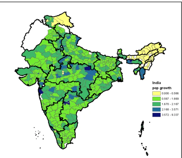
This number represents an increase of almost 80 percent in the urban population over this period. These figures mask large variability in urbanization patterns at the sub- national level; in particular, districts have urbanized at very different rates (figure S3.1a in the supplemental appendix, available at http://wber.oxfordjournals.org/). For instance, a district such as Idukki in Kerala increased its urban population by 13,000 (+29 percent) between 1981 and 2001, whereas the urban population increased by 1.6 million (+416 percent) in Rangareddi (Andhra Pradesh) and by 2.4 million (+130 percent) in Pune (Maharashtra) over the same period. In the subsequent analysis, we attempt to exploit this variability to identify the impact of urbanization on rural poverty.
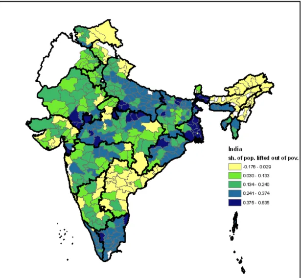
India also provides an interesting case in terms of the policy environment and economic performance given the structural changes in economic policy, the rate of growth, and the poverty levels experienced by the country during this period. Despite disagreements regarding the extent to which economic growth increased the welfare of India’s poor, poverty in India declined steadily in the 1990s, particularly in rural areas (Kijima and Lanjouw 2003). The geography of the decrease in the share of the poor, however, is extremely varied (figure S3.1b in the supplemental appendix,
population was lifted out of poverty in many districts between 1983 and 1999, for approximately a quarter of the districts, the incidence of poverty has remained roughly constant or has worsened over the same period.
India is the country with the largest number of both rural and urban poor.
India’s number of $1/day rural poor in 2002 was over 316 million, representing 36 percent of the world’s rural poor. The country is expected to add a further 280 million urban dwellers by 2030.3 Thus, estimating the impact of urbanization on rural poverty in India can help to identify the potential effects of this expected growth of the urban population on the world’s largest stock of rural poor. Our results suggest that urban growth has a significant poverty-reducing effect in rural areas within the same district, explaining between 13 percent and 25 percent of the overall decrease in rural poverty over the period.
The rest of the paper is structured as follows. The next section identifies the possible channels through which urban population growth affects rural poverty.
Section two describes the data used. Section three details the empirical methodology employed, including the variables used and the strategy to distinguish location and economic linkage effects. Section four presents the results, and section five concludes.
<<A>>Urban-rural linkages
We can draw from existing theoretical and empirical insights to identify the main mechanisms underlying the economic linkage effects of urbanization on economic conditions in nearby rural areas. There are at least six channels through which urban population growth can affect rural poverty in surrounding areas: consumption linkages, rural nonfarm employment, remittances, the rural land/labor ratio, rural land prices, and consumer prices.
<<B>>Consumption linkages
An expanding urban area will generate an increase in the demand for rural goods. This channel is likely to operate via an income effect as well as a substitution effect. The income effect is related to increased demand for agricultural goods due to higher (nominal) incomes in urban areas relative to rural areas. This phenomenon was documented as early as the Industrial Revolution; Allen (2009) describes how trade and proto-industrialization in British cities increased the urban consumption of goods produced in the countryside. This higher income is explained by urbanized economies: urban areas have denser markets for products and factors, which increase labor productivity and wage levels over the levels of rural areas (Duranton and Puga, 2004). The substitution effect is related to the increased share of higher value-added products in total agricultural demand that is typical of more sophisticated urban consumers. Empirical evidence from India and Vietnam confirms this composition effect (Parthasarathy Rao et al. 2004; Thanh et al. 2008). As noted below, we expect these effects to grow stronger closer to urban areas as a result of the weakly integrated agricultural markets within India (Jha et al. 2005).
<<B>>Rural nonfarm employment
Expanding urban areas can also favor the diversification of economic activity away from farming, which typically has a positive effect on income (e.g., Berdegue et al. 2001; Lanjouw and Shariff 2002; Jacoby and Minten 2009). This effect is particularly important in the rural areas surrounding the cities. Three concomitant effects can explain this increased diversification. First, proximity to cities may allow some of the peripheral urban workforce to commute to the city to work. Commuting, in turn, generates suburban nonfarm jobs in services, such as consumer services and
cities provide dense markets to trade goods and services more efficiently, rural households close to cities can afford to specialize in particular economic activities (because of their comparative advantage), relying on the market for their other consumption and input needs (Fafchamps and Shilpi 2005; Dercon and Hoddinot 2005). This more extensive specialization is likely to boost productivity and income (Becker and Murphy 1992). Third, proximity to urban areas stimulates the nonfarm activities that are instrumental to agricultural trade (which is increased by urbanization), such as transport and marketing. Recent evidence from Asia provides strong support for the effect of cities in stimulating high-return nonfarm employment in nearby rural areas (Fafchamps and Shilpi 2003; Fafchamps and Wahba 2006;
Deichmann et al. 2008; Thanh et al. 2008).
<<B>>Remittances
Remittances sent to rural households of origin by rural-urban migrants constitute another potentially important economic linkage effect of urbanization on rural poverty. The vast majority of rural-urban migrants (between 80 percent and 90 percent) send remittances home, with varying proportions of income and frequency (Ellis 1998). To the extent that urbanization is (partly) fuelled by rural-urban migration, this growth may be associated with larger remittance flows to the rural place of origin. Stark (1980) and Stark and Lucas (1988) provide evidence in support of the positive effects of remittances in reducing resource constraints for rural households and providing insurance against adverse shocks (because their income is uncorrelated with the risk factors of agriculture).4
<<B>>Rural land/labor ratio
Urbanization and rural poverty may also be linked through the changes in the rural labor supply that accompany the urbanization process. To the extent that rural-
urban migration reduces the rural labor supply, this reduction would increase (reduce the decrease of) the land available per capita in rural areas. Given a fixed land supply and diminishing marginal returns to land, this increased availability should increase labor productivity in agriculture, creating some upward pressure on rural wages.5 There is evidence in India of an association between out-migration from rural areas and higher wages in the sending areas (Jha 2008).6
<<B>>Rural land prices
The growth of cities can increase prices of agricultural land (owned by farmers) in nearby rural areas as a result of greater demand for agricultural land for residential purposes. This increase may generate increased income for landowners through sale or lease or through enhanced access to credit markets, where land acts as collateral. Some evidence from the US indicates that the expected (urban) development rents are a relatively large component of the agricultural land values in US counties that are near or that contain urban areas (Plantinga et al. 2002). The consumption linkage channel of urbanization described above can also be expected to increase land rental prices as a result of a rise in the expected future stream of income from agriculture. The impact on rural poverty through this channel depends on how this increased income is distributed across the rural population. Typically, if land is very concentrated, this channel is likely to benefit a few landowners, potentially restricting access to waged agricultural employment for the landless population.
Given the constraints on the reallocation of agricultural labor across sectors and the high labor intensity of agriculture, we would expect the net effect on rural poverty to be adverse (i.e., an increase in rural poverty) when land is highly concentrated (and vice versa).
Because the growth of a city is associated with lower consumer prices, surrounding rural consumers who have access to urban markets may benefit through higher real wages (Jacoby 2000). This effect may be due to increased competition among a larger number of producers in the growing urban area as well as thicker market effects in both factor and goods markets (Fujita et al. 1999). However, the increased demand for agricultural goods may also lead to higher prices for these goods, especially if the supply is fairly inelastic. Therefore, the direction of the net effect of urbanization on consumer prices is a priori ambiguous.
This study predicts that the total net effect of urbanization on rural poverty is poverty reducing. Moreover, the bulk of the effect is expected to be felt in rural areas that are relatively close to the growing urban area. This distance decay effect is consistent with recent research on the welfare impact of the expansion of a gold mine in Peru (Aragόn and Rud 2009) and is important for our identification strategy, as explained below. The next sections will detail the methodology used to test these hypotheses by measuring the total net effect in the case of Indian districts.
<<A>>Data
The data for the empirical analysis come from three main sources. For the district-level measures of poverty, we use data from three “thick” rounds of the National Sample Surveys (NSS: the Indian household survey) spanning the 1980s and the 1990s, the 38th (1983–84), 49th (1993–94) and 55th (1999–2000) rounds of the NSS.7,8 These measures have been adjusted by Topalova (2010) in two ways. First, she uses the poverty lines (based on the state-level prices computed separately for rural and urban areas) proposed by Deaton (2003a, 2003b) instead of the standard Indian Planning Commission poverty lines, which are based on defective price indices. Second, she adjusts the consumption data from the 55th round to
accommodate for a change in the survey design vis-à-vis the previous rounds (i.e., the recall period for certain goods).9
We are aware that the reliability of the district-level estimates of urban poverty is widely debated in light of the relatively small number of sampled households (Hasan et al. 2007; Topalova 2010). Although we use the urban poverty measure at the district level, the results are also robust to using urban poverty at the level of the NSS regions, which are a census-based aggregation of several districts (there are approximately 60 NSS regions in India).10 To the extent that the limited representativeness at the district level can be considered a classic nonsystematic measurement error in the dependent variable, it should not bias the estimate of the coefficients. It only suggests lower efficiency.
The other district-level data, such as population composition, come from the Indian districts database at the University of Maryland (which has been extracted from the original data in the Indian Census), which we update to 2001 using data from the Indian Census.11 Data on town populations are available from various rounds of the Indian Census. In addition, for crop production volumes and values, we use the district-level database for India, available from the International Crops Research Institute for the Semi-Arid Tropics from 1980 to 1994 and recently updated to 1998 by Parthasarathy Rao et al. (2004).12
The district classification was modified during the period of analysis because some districts were split into two units. Topalova (2010) created a consistent classification by aggregating the 2001 districts that originated from the district division of 1987. We conform to this reaggregation and modify the original population and demographic data accordingly.
<<A>>Empirical strategy
We attempt to systematically assess whether and to what extent the urbanization in Indian districts during the 1983–1999 period affected rural poverty in these districts. We argue that districts are an appropriate spatial scale for such an analysis in India because all of the location and economic linkage channels described above are likely to display most of their effects within a district’s boundaries. This argument is consistent with the theoretical discussion above suggesting that the effects of city growth are concentrated in surrounding rural areas. Specific evidence on India confirms that this relationship is likely to be the case.
First, intradistrict migration in India is a large component of total rural-urban migration. According to the census (Government of India 1991), 62 percent of the total stock of permanent internal migrants was intradistrict in 1991, although a share of this stock was composed of women migrating for marriage reasons.13 This statistic does not deny the existence of long-distance migration in India, which increased during the 1990s (Jha 2008). However, long-distance rural-urban migration is primarily directed at a few growing metropolitan areas, such as Mumbai, Delhi, Bangalore, and Chennai, which are excluded from the analysis for this reason.14 Notwithstanding the importance of intradistrict migration, in the empirical section, we test the robustness of the results against the relative size of the intradistrict migrant population.
Second, during the period of analysis, most agricultural goods markets do not appear to be well integrated at the national or even at the state level in India. The extremely poor transport infrastructure is one of the largest obstacles to trading bulky agricultural goods throughout the country (Atkin 2010). Furthermore, India maintains high internal food-trade barriers, including tariffs at state borders, licensing
requirements for traders and district-level entry taxes (Das-Gupta 2006). Thus, a consistent share of agricultural trade tends to occur at a short distance, making districts a suitable spatial scale to capture a substantial part of the first two channels.
Consistent with these ideas, some studies have tried to capture the demand-side effects on agriculture through district-level analyses (Parthasarathy Rao et al. 2004).
There is also emerging evidence of increases in land prices in peri-urban and rural areas surrounding the urban agglomerates. The land values in these areas may be well above the discounted future stream of income from agricultural activity, inducing some landowners to sell the land (Jha 2008).15
We begin from the following basic specification:
dt dt U
j dt st d R
dt P X
H =α +λ +β − +χ +ε
, (1)
where HdtR is a measure of rural poverty in district d at time t, α is the district fixed effect, λ is the state-year fixed effect,PdtU−jis the urban population of district d at time t-j (where j∈[1,2]), and X is a vector of controls that includes other variables that are likely to have an independent impact on rural poverty, including, inter alia, the district’s rural population to control for the growth of the district’s overall population.
The coefficient of interest here is β, which measures the collective impact of the location and economic linkage effects of urbanization on rural poverty.
We use a standard Foster Greer Thorbecke (FGT) measure of poverty for HdtR, the poverty headcount ratio. PdtU−j, the main independent variable, is computed as
∑
= −= Nd
i d
j it U
dt u
P
1
, where uitd−j is the population of town i in district d at time t-j and Nd is the number of cities in district d. Because population figures from the census are
available with only a 10-year frequency (e.g., 1981, 1991, 2001), the data for 1997 are estimated through nonlinear interpolation.16
The two sets of fixed effects included in (1) absorb some of the unobserved heterogeneity likely to bias the estimation. In particular, the district fixed effects absorb any time-invariant component at the district level, such as geographical position, climatic factors, and natural resources. The state-year fixed effects capture any state-specific time-variant shocks (including economic dynamics and policies).
This specification, however, may not completely account for other sources of potential bias in the coefficient β, including endogeneity. For this reason, in the next section, we address a number of possible remaining concerns by means of several robustness tests and instrumental variable (IV) estimations.
<<B>>Disentangling economic linkage from location effects
As mentioned above, it is important to empirically distinguish the economic linkage effects from the simple composition effect due to the migration of the poor from rural to urban areas (location effects) when identifying the impact of urbanization on rural welfare. To disentangle these effects, we start from the observation that a district’s urban population grows more rapidly than the rural population because of two phenomena: intradistrict rural-urban migration or rural areas becoming urban (either because they are encompassed by an expanding urban area or because their population has grown sufficiently to upgrade from the status of village to that of town).17 These two phenomena directly change the composition of both the rural and the urban populations, including their poverty rates. If the distribution of rural-urban migrants is skewed toward low-income individuals (i.e., the incidence of poverty is higher among migrants than nonmigrants) and if the poverty incidence in rural villages that become urban is higher than it is in the total rural
population of the district, then rural-urban migration will directly reduce rural poverty. This example demonstrates the poverty-reducing location effect of urban growth.
To properly isolate the location effects of urbanization on rural poverty, we need representative data on the poverty profile of rural-urban migrants and the dwellers in areas that are rural at time t-1 and that become urban at time t.
Unfortunately, these data are not available for the Indian context. Thus, we must find indirect proxies for this information.18
We use two sets of variables for this purpose. The first set is composed of three rural socio-demographic variables: the number of rural people in the 15–34 year age group, the share of literates in this group, and the share of the rural population classified as scheduled caste. The rationale behind the inclusion of these variables as proxies for the location effects of urbanization relies on the assumption that the poverty distribution of migrants can be expressed as a function of the migrants’ age, literacy, and caste composition. Other things being equal, the incidence of poverty tends to be lower among young adults (i.e., 15–34 years old) because they represent the most productive age class.19 Therefore, the higher the share of young adults in the total migrant population (relative to their share in the rural population), the lower the probability is that urbanization will directly reduce rural poverty. Because we do not observe the composition of the migrant population, we can only control for it indirectly through the composition of the actual rural population. This strategy relies on the plausible assumption that the change in the number of young adults in the rural population is inversely related to the change in their number among the rural-urban migrant population in the same period.20 The same argument can be applied to literate
migrants, whereas the reverse is true for scheduled caste members, whose poverty incidence is higher than that of the rest of the population.
The second type of variable capturing the location effects of urbanization is the urban poverty rate. Changes in this variable should indirectly reflect the poverty profile of rural-urban migrants in every period. This hypothesis follows from the fact that the probability that poor rural-urban migrants will become urban poor (after migrating) is higher than the same probability for nonpoor rural-urban migrants.
Therefore, for any given level of urban economic growth (which is the main determinant of urban poverty) between t and t-1, urban poverty is more likely to decrease between t and t-1, with a lower share of rural poor migrating to urban areas during that period.
In addition, the urban poverty rate can control for some unobserved time varying district-specific shocks that can affect both rural poverty and the urban population. For example, there may be a localized shock that spurs the district’s economic growth. Because economic growth is generally associated with urbanization, this growth can foster urbanization while simultaneously reducing rural poverty. This omitted variable problem implies a spurious negative association between the two variables. The data on income per capita at the district level are not available to us. However, because a district’s economic growth is likely to be the main determinant of the evolution of urban poverty (as well as rural poverty) in that district, and to the extent that the poverty-reducing effects of economic growth are similar across urban and rural areas, the urban poverty rate is a good proxy for a district’s economic growth.
Because the main aim of this paper is to estimate the size and direction of the economic linkage effects of urbanization on rural poverty, we can now extend (1) to separately capture the location effects of urbanization:
dt dt U
dt dt U
j dt st
d R
dt P Z H X
H =α +λ +β' − +Γ +γ +χ +ε
, (2)
where Z is the vector of socio-demographic variables described above and HUdt is the urban poverty rate. To the extent that these additional variables capture the location effects, β’ measures only the economic linkage effects of urbanization on rural poverty. This coefficient should thus quantify the collective effect of the urban-rural linkages described in section two. Because all of these linkages point toward the rural poverty-reducing effect of urban growth, β’ is expected to be negative. The empirical analysis below attempts to disentangle the effects of some of these economic linkage channels. The difference between β in (1) and β’ in (2) should be an indication of the size and direction of the location effects of urban growth on rural poverty.
There may be some concern that urban poverty could be endogenous in expression (2) because it is simultaneously determined with rural poverty. To relieve these concerns, we employ a variant of this specification without urban poverty that uses the number of urban nonpoor instead of the number of urban people as the main regressor:
dt dt dt
NP U
j dt st
d R
dt P Z X
H =α +λ +β'' −( )+Γ +χ +ε
. (2’)
Given the property of urban poverty discussed above, we would expect the coefficient of the number of urban nonpoor to more closely capture the economic linkage effects of urbanization on rural poverty (coefficient β’’) than the β coefficient of the total urban population in (1), which captures the overall effect of urbanization on rural
less affected by the quantity of poor rural-urban migrants (who are more likely to become urban poor, at least in the short term) than the total urban population variable.
Again, the difference between the standardized coefficients of the total urban population β and of the urban nonpoor population β’’ provide a sense of the magnitude of the location effects.
<<A>>Results
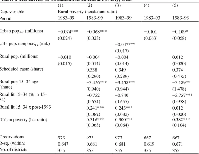
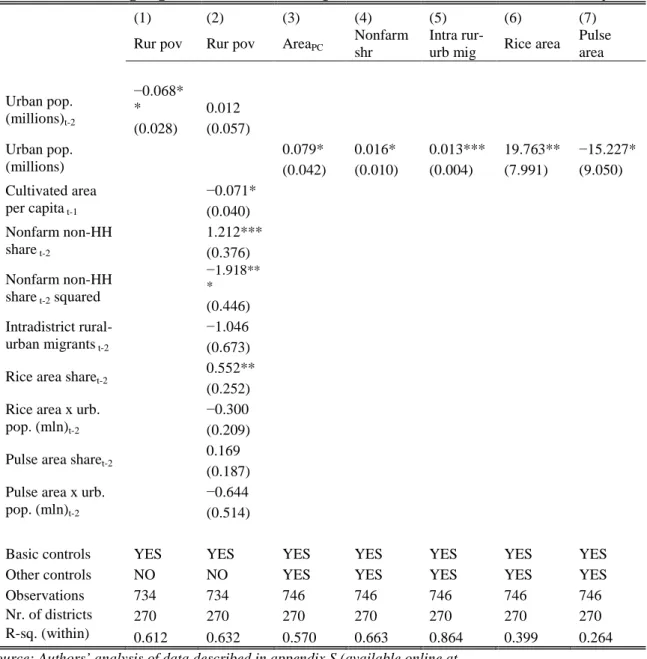
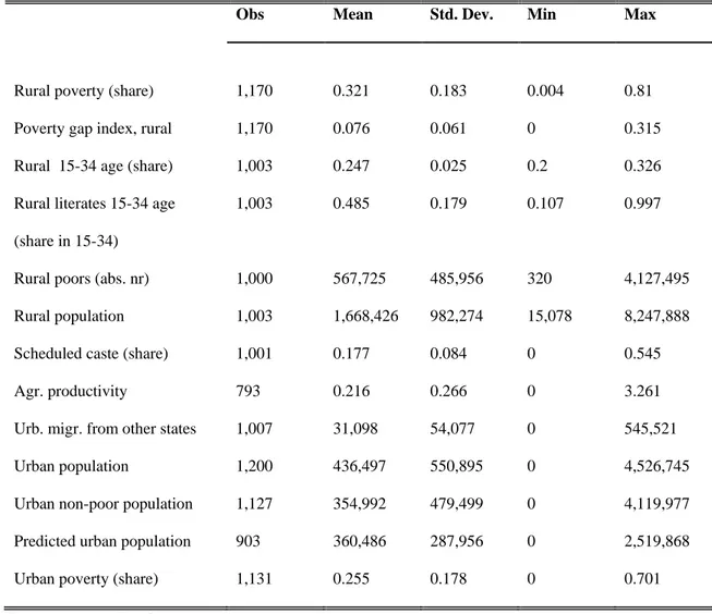
The descriptive statistics for the main variables used in the analysis are presented in table S2.1 (available online at http://wber.oxfordjournals.org). Table 1 presents the results of specifications (2) and (2’) using fixed effects estimation. Our dataset includes observations of 363 districts for three different time periods: 1983, 1993, and 1999. We run the regressions applying a two-year lag to the measure of the urban population and to the other demographic controls for two primary reasons.
First, the two-year lag reduced the risk of potential simultaneity bias. Second, the two- year lag allows us to limit the use of interpolation for the Census variables (both population and socio-demographic variables), which are recorded in 1981, 1991 and 2001, to the last period (1999) only.21 The standard errors are robust to heteroscedasticity (using the Huber-White correction) and are clustered at the district level.
<<Table 1 about here>>
The estimate in column 1 indicates that the growth of the urban population exerts a significant poverty-reducing effect on the rural areas in the same district. This result is obtained by including district and state-year effects as well as the total rural population and should capture the overall effect of urbanization on rural poverty.
Column 2 adds the set of controls, which, as we have argued above, should capture
most of the location effects of urbanization. The coefficient of the urban population is virtually unaffected by the inclusion of these controls, suggesting that most of the poverty-reducing effect of urban growth is due to economic linkage effects. This finding is consistent with the evidence that rural-urban migrants (including those within the same district) enjoy, on average, similar, albeit slightly higher, expenditures and education levels than the rural stayers in India (Singh 2009). This similarity is also the case in Tanzania (Beagle et al, 2011). Even if our controls imprecisely capture the location effect of urbanization on rural poverty, this evidence suggests that our estimation would tend to underestimate the absolute magnitude of the economic linkage effect of urbanization on rural poverty.
This magnitude over the 1983–1999 period is not particularly strong, according to our estimate. An increase in the district’s urban population of 200,000 (a 43 percent increase from the mean value) reduces the poverty rate by approximately 1.3 percentage points, on average. Over the period of analysis, the rural poverty rate decreased by approximately 20 percentage points, and the urban population increased by 400,000 in the average district. Therefore, urban growth is responsible for approximately 13 percent of the overall reduction in rural poverty in India during the 1983–99 period.
When we use the nonpoor urban population as the main regressor, the β1
coefficient decreases by approximately one-third vis-à-vis the total urban population coefficient (column 3). However, when considering the urban nonpoor effect in proportionate terms, the two effects are basically identical, providing further confirmation that the economic linkage effects of urbanization on rural poverty drive the overall poverty-reducing impact of urbanization in rural areas.
The signs of the controls are as expected, except for the positive coefficient of the share of literates in the last period (i.e., post-1993), when a higher incidence of literates in the most productive part of the rural labor force was associated with higher levels of rural poverty. A higher share of young adults in the rural population decreases rural poverty, whereas a higher presence of scheduled caste increases it (although not significantly). This result suggests that the direct effect of the young adult population on poverty prevails over the indirect effect, which captures the rural- urban migration of young adults. The inclusion of the controls does not significantly change the urban population coefficient.
One possible concern with these results is that the demographic controls, including the urban population, are interpolated for the last period. To address this issue, we check the robustness of our results when we restrict the analysis to the first two periods covering the 1983–1993 time interval because no interpolation is needed in this case. This analysis is interesting in its own right because it focuses only on the preliberalization period. Overall, the effect of urbanization on rural poverty is slightly stronger over this period than over the entire period (columns 4 and 5), although the difference in the coefficients is not statistically significant. Again, the bulk of the effects appear to be driven by economic linkage effects (cf. column 4 vs. 5).
Furthermore, both the share of young adults in the rural population and the share of literates in the young adult population are associated with a reduction of rural poverty.
This association supports the hypothesis of a differential impact of literacy on rural poverty over time: it is poverty reducing until 1993 and then is poverty increasing.
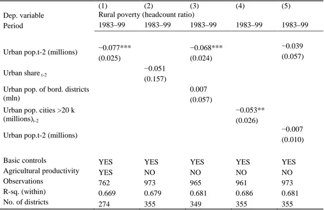
<<B>>OLS: further robustness
The analysis thus far does not completely account for other sources of potential bias in the coefficient of interest β’. Table 2 presents the results of a battery of tests to check the robustness of the results to a number of these possible concerns.22
A first potential source of bias is related to the omission of agricultural productivity. As argued by some of the literature on structural transformation, agricultural productivity growth can drive both urbanization and rural poverty (e.g., Matsuyama 1992; Michaels et al. 2012). To address this issue, we add the measure of agricultural land productivity to the list of controls in column 1. The variable is constructed as the sum of the total value of 22 different crops produced in a given district divided by the area cultivated with these crops. To estimate the value, we use India-wide crop-specific prices instead of district prices to minimize data gaps (of which there are several for the latter) and the potential endogeneity of the districts’
prices to rural poverty.23 The variable is lagged one year because the simultaneity bias should not be an issue in this case, but a contemporaneous specification is not possible because of the lack of data for 1999. The main results are robust to the inclusion of this measure, which turns out to be not significant.24
Second, a question remains regarding the extent to which the impact on rural poverty can be attributed to composition (urban versus rural) rather than simply to a scale effect. To check for this, we substitute the urban population with the share of the urban population in the total population as the main regressor (column 2). This specification is close to Ravallion et al. (2007) and yields a negative, although not significant, urban coefficient. This result suggests that the (economic linkage) effects of urbanization on rural poverty are primarily driven by a scale effect rather than a
Third, until now, the estimation strategy has made the implicit assumption that the towns in a district are centrally located. However, in practice, they are neither centrally located nor evenly distributed within a district. This assumption could therefore lead to a biased estimation. For example, if a district has a large city just outside of its border, the relationship between rural poverty and urbanization within this district could simply be driven by the population growth in the city. Although we include district-level fixed effects and state-specific time effects in the regressions, this source of omitted variables may persist because of the growth of the city in the surrounding district over time. To address this concern, we add to the set of controls a spatially lagged urbanization variable, the average of the urban population of the contiguous districts (column 3). The results are once again unaffected, and this extra control is not significant.
Fourth, a further possible bias of our analysis may be due to small villages that upgrade to towns in the census definition. To the extent that these growing villages are systematically located in rural areas where poverty is decreasing (increasing) for reasons independent of urbanization, we might detect a spurious negative (positive) effect for the urban population on the poverty share. We therefore reestimate the models, excluding from the urban population the variable towns with fewer than 20,000 inhabitants, the size category that would contain most of the ‘upgraded villages.’ Again, the results of this regression are extremely similar, although slightly less precise (column 4).
Finally, we might think that the effect of the urban population on rural poverty may be nonlinear. In this case, our model would be misspecified. We test whether nonlinearity is the case by adding the square of the urban population as an explanatory variable whose coefficient, however, is close to zero and not significant (column 5).
We also attempt different specifications, substituting the urban population variable with various variables corresponding to the sum of the urban population by the size class of the towns (we attempt a number of different size classifications). Again, all of these additional variables have statistically nonsignificant coefficients (results not shown but available from the authors upon request), leading us to conclude that the linear approximation is substantially adequate to identify the phenomenon under scrutiny.
<<Table 2 about here>>
<<A>> IV Estimation
Despite addressing these concerns, the estimation of (2) could still be biased to the extent that the relationship between rural poverty and the urban population is characterized by reverse causation; the conditions in the rural sector affect urbanization, or there is a correlation of unobserved variables with the variable of interest.
In particular, we are concerned that rural poverty could drive rural-urban migration. Rural poverty could either act as a push factor (i.e., poorer people migrate in search of an escape from poverty), or in the presence of the high fixed costs of migration, it can act as a restraint to migration. If the former case dominates (i.e., poverty is primarily a push factor), the coefficient β’ in (2) would have a downward bias, whereas the opposite is true if the latter effect of poverty on migration dominates. The findings by Ravallion et al. (2007) that associate global rural-urban migration with a large reduction in the number of rural poor lends some credit to the prevalence of the former case. Kochar (2004) also provides indirect support for this hypothesis, showing that in India, landless households have the highest incidence of
We resort to an IV estimation to address the endogeneity bias. To that end, we need at least an additional variable to act as a valid instrument, one that is correlated with the district urban population and exogenous to the poverty-induced rural-urban migration flows. We identify three variables that could plausibly satisfy both conditions and are candidates for valid instruments.26
The first variable is based on the fixed coefficient approach (Freeman 1980;
Card 2001; Ottaviano and Peri 2005) and uses national levels of the urban population and the lagged values of its distribution across districts. This instrument builds on the interaction between two sources of variation, which are exogenous to changes in the local characteristics influencing urban population growth at the district level: the initial distribution of urban population across districts and the national trend in urban population. Similar to Card (2001), Ottaviano and Peri (2005), and Cortés (2008), we define the instrument for district d in year t as the share of the urban population of district d in the total Indian urban population in 1971 multiplied by the total urban population in India at time t:
∑
∗∑
= d
U dt d
U d U U d
dt P
P
Pˆ P ( )
1971 1971
.
(3)
The predicted measure defined in (3) conveys the size of the urban population in each district that would have been observed if the distribution of the urban population across districts had not changed since 1971. The fact that the initial urban population distribution is referred to 10 years before the beginning of our analysis reinforces its exogeneity to changes in the district urban populations during the period under scrutiny. In a cross-sectional setting, this exogeneity would not necessarily hold true; the unobserved structural factors driving the urban population dynamics before
1971 could also affect rural poverty in later periods. In our panel analysis, however, all of the regressions include the district fixed effects, which absorb all of the time- invariant factors at the district level and therefore the long-term determinants of urban growth. The hypothesis of serial correlation in the rural poverty variable is also unlikely because India underwent many political, social, and economic changes in the 1970s and 1980s, which make it extremely unlikely that the district-specific dynamics in the 1950s and 1960s, for example, would be serially correlated with the rural poverty dynamics in the 1980s and 1990s (after conditioning on state-year fixed effects). However, the contemporaneous India-wide trend in urban population is safely exogenous to the district-specific changes in rural poverty.
Moreover, because the strategy adopted for the first instrument is not immune to criticism (e.g., Cortés 2008), we also employ two other instruments. The first additional instrument is the number of people who migrate to the urban areas of the district from states other than the state where the district is located. It is plausible to assume that rural poverty or the other push factors for migration in the other states are uncorrelated with the district characteristics once we control for the state-year fixed effects. At the same time, the number of migrants coming to district towns from other states is part of the urban population of the district and thus has a positive association with our main explanatory variable. Nevertheless, a concern about the exogeneity of the instrument could arise from the fact that, within a given district, the time-varying urban pull factors can be correlated with time-varying rural pull factors, and the latter can, in turn, be correlated with rural poverty. For example, migration from other states to the urban areas of one district could be driven by an unobserved positive shock to the entire district, such as an increase in government funding. This shock would help
to reduce poverty throughout the district, effectively invalidating the exclusion restriction of our instrument.
However, the first (and second) stage of the IV estimation includes all of the controls listed in the ordinary least squares (OLS) specification, and some of them are good proxies for the pull factors of migration to the district rural areas: the measure of agricultural productivity, the demographic characteristics of the rural population, and the interaction of time and state fixed effects. To further address these concerns, we add the number of migrants from other states to the rural areas as a control. This variable should capture any district or rural district shocks driving both migration and poverty. The results with this additional control are nearly identical to the others.27 Therefore, we can assume that the second IV captures the effect of migration to district cities from other states, conditioning out the pull factors of district rural areas.
The last instrument is based on the recognition that the urban areas that are relatively more specialized in tradable sectors are more likely to reap the benefits of Indian economic liberalization, which greatly facilitated trade within and outside of India (Aghion et al. 2008; Topalova 2010). Therefore, the cities that specialized in the tradable sector (proxied by manufacturing) before the liberalization shock were more likely to experience a positive trade shock, leading to faster population growth (primarily through immigration). Therefore, we develop an additional instrument based on the interaction of the manufacturing share in urban employment in 1981 with a postliberalization dummy (equal to one for all the years following 1993). The validity of the instrument is further reinforced by the inclusion of the rural manufacturing share in the control set. The rural manufacturing share controls for the possibility that the instrument could reflect the economic structure in the district’s rural area, thus capturing some of the direct effect of liberalization on rural poverty.
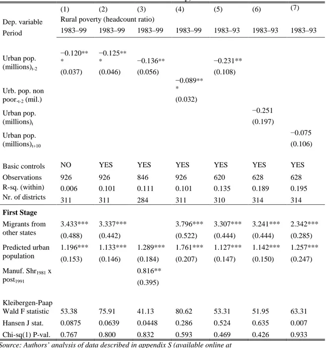
Columns 1 to 5 of table 3 present the results of the estimations using these instruments. Because the inclusion of the three instruments together leads to a weaker first stage, we included the strongest ones—migrants and predicted population—in all regressions except column 3, in which the migration instrument is substituted with the postliberalization instrument. In all cases, the first-stage coefficients substantiate the power of the instruments, with a Kleibergen-Paap Wald F-statistic well above the confidence threshold of the Stock and Yogo (2005) test for weak instruments.
Furthermore, the test of the overidentifying restrictions (Hansen’s J, reported in the last two rows of table 3) supports the exclusion restriction assumptions for all IV specifications. Analogous to OLS, the standard errors in the IV estimations are robust and clustered at the district level.28
<<Table 3 about here>>
The results from the second-stage regressions confirm those of the OLS regression, including the significant reducing impact of urbanization on rural poverty and the fact that most of this impact is driven by economic linkage effects. The main difference between these regressions concerns the absolute size of the urban population coefficient, which is almost twice as large as the OLS estimate (and over twice as large in the case of the 1983–93 period). According to the IV estimation, an increase in the urban population of 200,000 reduces rural poverty by between 2.4 and 2.6 percentage points, and urban growth was responsible for approximately one- quarter of the total rural poverty reduction during the 1983–99 period. The larger urban coefficient in the IV estimation is consistent with our theoretical expectations.
An attenuation bias in the OLS regression could be due to a favorable shock in rural areas, which reduces rural poverty, rural-urban migration, and thus the urbanization
absolute size of the coefficient. The larger IV coefficient could be due to measurement error in the endogenous variable.
<<B>>Falsification test
To further support the validity of our IVs, in columns 6 and 7 of table 3, we report a falsification test based on the assumption that we should not find an effect of future urban population on rural poverty in the two-stage specifications. On the contrary, if the coefficient of the future urban population is significant, this implies a district-specific trend that is correlated with both rural poverty change and urbanization, which makes the IV estimates inconsistent.
Such a test, however, cannot be directly implemented because the available urban population is lagged two years with respect to rural poverty in the data.
Therefore, there is a partial temporal overlap of the two variables, even if the urban population is referred to the subsequent period (e.g., rural poverty in 1983–1993 regressed on the urban population in 1991–2001). Therefore, we use the contemporaneous variable for the years 1981 and 1991 (plus 2001 for the future urban population), and we extrapolate the poverty data for those years using the 38th round and the 43rd round of the NSS survey, conducted in 1983 and 1987, respectively. In this way, we are able to exploit the variation in rural poverty that does not overlap in time with the variation in the urban population. In all other aspects, including the control variables and instruments, the regressions are identical to those reported in column 5 of table 3.
The results from the contemporaneous specification are qualitatively similar to those shown in column 5, with an even larger coefficient (−0.25), which is significant at the 80 percent level (the lower significance is probably due to the interpolation, which adds some noise to the dependent variable). When we substitute the urban
population with the future values (10 years later), the coefficient is much smaller (−0.07), with standard errors that are 50 percent higher than the coefficient value (0.11). This finding supports the assumption that the instruments are exogenous to a district-specific trend, potentially affecting both urban population growth and rural poverty dynamics.
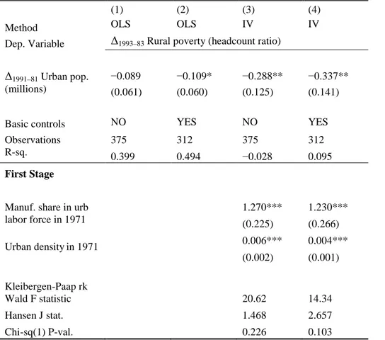
<<B>>First differences estimation
Given the importance of rigorously addressing the potential endogeneity bias in this type of analysis, we employ a different instrumentation strategy. We conduct an analysis of first differences instead of through fixed effects, regressing the change in rural poverty on the change in the urban population and the other control variables.
In this way, we are able to exploit the determinants of urban growth as instruments. In particular, we use two determinants that have proven to be important in the literature (Glaeser and Shapiro 2001; Glaeser and Saiz 2004): the share of manufacturing employment in the urban adult population in 1971 and the historical (1931) urban population density. Manufacturing employment has been shown to be an important determinant of subsequent urban growth in societies at relatively early stages of industrialization, such as the United States in the first part of the 20th century (Glaeser et al. 1995). Manufacturing specialization became negatively associated with urban growth as economies moved away from industries and toward tertiary sectors, as occurred in the United States at the end of the last century (Glaeser and Shapiro 2001). It is plausible that India, during the period of our analysis, could be considered an economy in the early days of the industrialization process, comparable to the United States in the first half of the 20th century. Hence, it could be supposed that manufacturing employment would be associated with subsequent urban growth in the
The second instrument in the first-difference estimation is the density of the urban population in 1931. The intuition here is that in a period of widespread urbanization across India, some districts were urbanizing relatively faster because their physical geography (e.g., terrain slope, water sources, railroads) was more suitable for urbanization. Because the effects of physical geography on urbanization are likely to be persistent over time and because these geographic factors do not change over time and were important for historical urbanization, the historical density of urban population is a good proxy for them.
Table 4 reports the results of the estimation of first difference. The results are strictly comparable to the fixed effects results for the 1983–93 period. The size of the IV urban population coefficient triples vis-à-vis its OLS counterpart (column 3 and 4 compared with column 1 and 2). This change is reassuringly similar to that experienced by the coefficient in the fixed effect regressions using a different set of instruments. The larger coefficients likely result because the instruments are now slightly weaker, although in the first-stage regression, their coefficients have the expected sign and are both significant. Even in this case, the Hansen test suggests that the instruments are correctly excluded from the second stage.
<<Table 4 about here>>
<<B>>Unpacking the economic linkage channels
So far, we have established that urban growth reduces rural poverty within the same district and that most of this impact is driven by economic linkage channels. In this section, we attempt to test the extent to which some of these channels explain the rural poverty reduction impact of urbanization. In section 2, we identified six main channels: consumption linkages, rural nonfarm employment, urban-rural remittances, rural land/labor ratio, rural land prices, and rural consumer prices. We can construct
variables to proxy four of these channels, but the district data on land and consumer prices are not available separately for rural and urban areas. We add these variables to both the baseline (as defined in (2)) and the IV specifications to obtain a sense of the relative importance of these channels.
To capture the consumption linkage effect of urbanization, we use crop- specific shares of cultivated land. We interact this share at the beginning of the period of our analysis with the urban population variable to test the impact of urbanization across districts on the basis of their production dependence on specific crops. This measure relies on the assumption that a district’s supply is a good proxy for urban demand. To identify the relevant crops, we first test for the relationship between urbanization and the main crops across Indian districts.29 Among the crops that display a significant relationship, we then select the relatively large crops, those with a share of total cultivated land above 5 percent throughout the period. These cultivations are most likely to affect rural economic livelihood.
These crops are rice (which covers, on average, 15 percent of the total cultivated land) and pulses (8 percent). These are important expenditure items for Indian households (Subramanian and Deaton, 1996). India is the world’s largest consumer and producer of pulses and is one of the largest consumers and producers of rice. This choice is reinforced by the results of Jha et al. (2005), who show that the rice market is not integrated within India. As shown below, our analysis suggests that urbanization is associated with an increase in the cultivation of rice and a decrease in the cultivation of pulses. Although the latter result is expected (because pulses are considered a relatively poor crop), the former result is surprising because rice is usually substituted with wheat and other food products as income rises. One reason
the consumption linkage of urbanization appears to operate mainly through an income effect (which increases the quantities of the usual crops) rather than a substitution effect.
We use census data to construct the share of rural employment in nonagriculture/nonhousehold activities, which should capture the rural nonfarm employment channel.30 Again, urban-rural remittance data are not available for the period of this analysis; therefore, we use the number of intradistrict rural-urban migrants as a proxy for the remittance channel. We also include the share of rural- urban migrants in the total rural population to control for the possible influence of rural poverty on migration.
Finally, we use the total cultivated area over the rural population as a direct proxy for the rural land/labor ratio channel. To the extent that urbanization increases the demand for agricultural goods, thus raising the return on land cultivation, this ratio can also capture part of the consumption linkages channel.
Column 1 in table 5 shows the coefficient of the urban population obtained by running specification (2) for the reduced number of observations for which all of the new variables are available. Adding the set of new variables brings the urban population coefficient to zero (column 2).31 All of the new variables have the expected sign, although rural nonfarm employment has a nonlinear effect on rural poverty. For relatively low shares of rural nonfarm employment (i.e., below 32 percent of total rural employment), increases in this share are associated with increases in rural poverty, whereas the opposite is true when nonfarm/nonhousehold employment is greater than the 32 percent threshold. This finding suggests that rural nonfarm activities tend to be more profitable than agriculture only when nonfarm activities represent a substantial part of the rural economy. When these activities are
relatively marginal, they are likely to be confined to petty trading and other low-yield, nontradable services (such as construction and rickshaw pulling). Nonfarm activities appears to be relatively marginal in most Indian districts (in 1999, only 14 percent of the districts had a rural nonfarm share of employment above 32 percent). Most of the nonfarm employment involves casual employment (daily wage) and self-employment, which tend to be associated with lower incomes and lower stability than regular employment (Lanjouw and Murgai 2009). In 1999, the latter represented only one- quarter of the rural nonfarm employment in India and was the category that grew the least during our period of analysis.
The effect of internal rural-urban migrants is negative, as expected, although it is only significant at the 11 percent level, suggesting that a rise in the number of migrants is associated with a reduction in poverty through the remittance channel.
Similarly, the cultivated area per rural population, which increases through urbanization, has a statistically significant poverty-reducing effect in rural areas.
Finally, the shares of rice and pulse cultivated areas have a positive association with rural poverty (although it is not significant for pulses), consistent with the relatively small margins that are typical of these crops. However urbanization has a higher, albeit only weakly significant, poverty-reducing effect in districts with relatively large rice and pulse cultivations (i.e., consumer linkages are stronger).
We repeat the same exercise using IV estimation. The results are almost identical for both the urban population and the variables’ coefficients.32
To substantiate our claim that urbanization reduces poverty through these channels, columns 3 to 7 show the significant effect of the urban population variable on each of these variables. Using the same specification and controls as in column 2,
we find that urbanization affects each variable positively and significantly, except for the share of the pulse area, which is affected negatively.
We check the relative contribution of each channel to the poverty-reducing effect of urbanization by adding each variable in turn to the specification in column 1.
According to this analysis, approximately three-quarters of the poverty-reducing effect of urbanization is accounted for by consumer linkages. Intradistrict rural-urban migration accounts for less than one-fifth, and the rural land/labor ratio and the rural nonfarm employment account for 4 percent and 3 percent, respectively. The small contribution of the latter channel is particularly surprising because rural nonfarm employment is often an important cause of rural poverty reduction (Berdegue et al.
2001; Lanjouw and Shariff 2002). This surprising result could be explained by considering that urbanization affects rural nonfarm employment positively and that the latter has an inverted-U effect on rural poverty in India.
<<Table 5 about here>>
Taken at face value, these results suggest that the other channels that we were not able to properly capture (i.e., rural consumer and land prices) are not likely to account for any of the poverty-reducing effect of urbanization on the rural areas within the district. This implication seems consistent with the ambiguous effects of these channels on rural poverty that were discussed in section 2.
<<A>>Conclusions
Do the poor in rural areas benefit from the population growth in urban areas?
If so, what is the size of the benefit? Despite the importance of these questions, little empirical evidence is available to provide adequate answers. We have attempted to address this gap by analyzing the effects of urbanization on rural poverty. Using data
on Indian districts from 1983 to 1999, we find that urbanization has a significant poverty-reducing effect on the surrounding rural areas. The results are robust to the inclusion of a number of controls and to the use of different types of specifications.
The results of the IV estimation suggest that the effect is causal and that the failure to control for causality downwardly biases the coefficient of urbanization. We find that an increase in the urban population of 200,000 determines a decrease in rural poverty in the same district of between 1.3 (lower bound) and 2.6 percentage points.
These figures represent between 13 percent and 25 percent of the overall reduction in rural poverty in India over the period. That amount is a substantial contribution, but it is lower than the contribution of another important change to the rural sector, i.e., the state-led rural bank branch expansion, which can explain approximately half of the overall decrease in rural poverty in India between 1961 and 2000 (Burgess and Pande 2005).33 However, the contribution of urbanization to rural poverty reduction is slightly higher than that of another important state rural policy in post-independence India—land reform, which explains approximately one-tenth of the rural poverty reduction between 1958 and 1992 (Besley and Burgess 2000).
Our analysis suggests that the poverty-reducing impact of urbanization occurs through economic linkage effects rather than through the direct movement of the rural poor to urban areas. This finding is not surprising given that rural-urban migrants appear to be, on average, less poor and more educated than rural nonmigrants. These economic linkage effects of urbanization on rural poverty are accounted for by four channels: consumer linkages (which explain most of these effects), urban-rural remittances, the changing rural land/labor ratio, and nonfarm employment.
These findings have a number of potentially important policy implications.
reduction. In fact, it is a popular tenet that investments in developing countries should be concentrated in rural areas to reduce poverty because the poor in developing countries are primarily concentrated there (see, for instance, World Bank( 2008)).
However, investments in rural areas are often onerous because substantial resources are needed to reach a population that is scattered among vast territories. To the extent that urbanization can have substantial poverty-reducing effects on rural areas, urban investments may become an important complement to rural investments in poverty- reduction strategies.
Second, our findings run counter to the popular myth that rural-urban migration may deplete rural areas, causing them to fall further behind. The relatively low rate of urbanization in India may be due to public policies that have not facilitated (and, in certain instances, have even constrained) rural-urban migration (Deshingkar and Start 2003). At the very least, this paper questions the appropriateness of this bias against rural-urban migration.
Although this paper has not addressed the issue of urban poverty, increasing urban populations imply that, in the future, urban poverty may become a main issue in its own right (Ravallion et al. 2007). Further research is needed to assess whether the growth of the urban population entails a trade-off between rural and urban poverty reduction.
NOTES
Massimiliano Calì (corresponding author) is research associate at the Overseas Development Institute, UK. His e-mail address is m.cali.ra@odi.org.uk. Carlo Menon is an economist with the OECD, Science, Technology and Industry Directorate and with the Bank of Italy.
The authors thank Andrew Shepherd, who inspired the main question of the research, and Henry Overman for their detailed comments on an earlier draft. Thanks also go to Kristian Behrens, Gilles Duranton, Giovanni Favero, Steve Gibbons, Vegard Iversen, Veena Jha, Guy Michaels, Elisabeth Sadoulet, Kunal Sen, Stephen Sheppard, Tony