Active matter: from collective self-propelled rods to cell-like particles

Active matter: from collective self-propelled rods to cell-like particles

Inaugural-Dissertation zur

Erlangung des Doktorgrads

der Mathematisch-Naturwissenschaftlichen Fakult¨at der Universit¨at zu K¨oln

vorgelegt von Clara Abaurrea Velasco

aus Zaragoza, Spanien

J¨ ulich 2018

Prof. Dr. Matthias Sperl Prof. Dr. Ulrich Schwarz

Tag der m¨ undlichen Pr¨ ufung: 07. Mai 2018

A mis padres, Jes´ us y Curra.

”Sometimes I sits and thinks, and sometimes I just sits.”

-A.A. Milne, Winnie-the-Pooh

Zusammenfassung

Aktive Materie umfasst Systeme, deren Komponenten kontinuierlich Energie aufneh- men und dissipieren. Aktive Systeme mit vielen Agenten zeigen ein sehr reiches und komplexes kollektives Verhalten auf vielen verschiedenen Gr¨oßenordnungen: Zytoske- lettfilamente, bewegliche Zellen, phoretische Mikroschwimmer, Fischschw¨arme und Vo- gelschw¨arme. Kleine ¨ Anderungen auf der Ebene des Einzelagenten k¨onnen sich rasch ausbreiten und auf lange Sicht entstehende Strukturen und Ordnung erzeugen. Zellskelett- Filamente und Motorproteine beispielweisse bilden aktive viskoelastische Netzwerke und B¨ undel, welche die Form und Bewegung von Zellen bestimmen. Bakterien, die mit niedriger Reynolds-Zahl schwimmen, bilden aktive Kolonien, in denen turbulente Dy- namik beobachtet wird. Wir untersuchen das kollektive Verhalten un die Dynamik von Bakterien und aktiven Filamenten mit Hilfe von Computersimulationen von selbstan- getriebenen St¨aben sowohl in Systemen mit periodischen Randbedingungen, als auch in Systemen mit r¨aumlicher Einschr¨ankung.

Phoretische Mikroschwimmer und genetisch ver¨anderte E. coli Bakterien zeigen einen dichteabh¨angig-reduzierten Antrieb. Wir untersuchen das kollektive Verhalten und die Dynamik von selbstangetriebenen St¨aben (SPRs) mit dichteabh¨angiger An- triebskraft. W¨ahrend SPRs mit dichteunabh¨angigem Antrieb Streifen und gigantisch- wurm¨ahnliche Cluster bilden, bilden SPRs mit dichteabh¨angig reduziertem Vortrieb Astern und polare B¨ander. Die dichteabh¨angige Verlangsamung verst¨arkt die polare Ordnung und Clusterbildung der St¨abe und induziert eine lotrechte Anordnung an den Clustergrenzen. Daher sind Regionen mit geringer Dichte in Clusterphasen nahezu leer von St¨aben. Dieses Ph¨anomen wird in Clusterphasen klassischer SPRs nicht beobachtet.

Wir untersuchen auch SPRs innerhalb von mobilen, starren, kreisf¨ormigen Begren- zungen, welche somit komplexe, selbstangetriebene, starre Ringe bilden. Die St¨abe sind am Ring verankert, k¨onnen jedoch entlang der Kontur des Rings gleiten. Dies erlaubt uns, Systeme mit Schub-, Zug- und Mischst¨aben zu studieren. Die Stabdynamik und die emergenten Strukturen bestimmen die Ringdynamik und Bewegung. Zudem vermit- telt die Ringmotilit¨at SPR-Clusterbildung. Aktive Brownsche Teilchen weisen f¨ ur kurze Beobachtungszeiten ein thermisches Diffusionsregime, f¨ ur mittlere Zeiten ein ballisti- sches Regime und f¨ ur lange Zeiten ein aktives Diffusionsregime auf. Die zus¨atzlichen internen Freiheitsgrade im komplexen, selbstangetriebenen Ring f¨ uhren zu einer Ge- samtringdynamik, die nicht durch das aktive Brownsche Teilchenmodell erfasst werden kann. Die Stab-Selbstorganisation f¨ uhrt zu komplexen Motilit¨atsmustern, wie Run- and-Tumble¨ und Run-and-CircleBewegungen. Diese Motilit¨atsmuster, werden auch bei beweglichen Zellen beobachtet.

In einem weiteren Schritt hin zur Modellierung der Zellmotilit¨at untersuchen wir

SPRs in mobilen, deformierbaren Ringen. Neben der Ringmotilit¨at spielt die Derfor-

mierbarkeit eine entscheidende Rolle f¨ ur die SPR-Ausrichtung und Clusterbildung. In

Abh¨angigkeit von der Aktivit¨at der St¨abchen und der Reibung zwischen dem Ring

und dem Substrat finden wir drei verschiedene Klassen von Ringformen: fluktuierend,

keratozyten¨ahnlich und neutrophilartig. Hier sind Zugkr¨afte an der R¨ uckseite der Rin-

ge von entscheidender Bedeutung f¨ ur die Erlangung von zell¨ahnlichen Formen und

der Austrittswinkel unabh¨angig vom Eintrittswinkel ist, was mit experimentellen Beob- achtungen von Keratozyten an Grenzfl¨achen zwischen glatten und mikro-strukturierten Oberfl¨achen ¨ ubereinstimmt. Dar¨ uber hinaus haben experimentelle Studien gezeigt, dass Substrateigenschaften, wie die Haftfestigkeit, die Form und Bewegung der Zelle stark beeinflussen. In ¨ Ubereinstimmung mit Experimenten zeigen Simulationen verformbarer Ringe an Reibungsgrenzfl¨achen Form¨anderungen und Ablenkungen der Bewegungsrich- tung der Ringe.

Unsere Simulationen beschreiben aktive Systeme mit stabf¨ormigen Komponenten,

deren Antrieb sich an die Umgebung anpasst. W¨ahrend SPRs mit dichteabh¨angiger

Verlangsamung teilweise das beobachtete Verhalten von Bakterien mit dichteabh¨angig-

reduziertem Antrieb erfassen, k¨onnen SPRs in einer ring¨ahnlichen Begrenzung als mi-

nimales, Weiche-Materie-Modell f¨ ur Zellmotilit¨at angesehen werden. Mit unseren Simu-

lationen k¨onnen wir systematisch den Einfluss verschiedener Parameter wie Zellantrieb

und Substrateigenschaften auf die Zellmotilit¨at charakterisieren. Obwohl unsere Mo-

delle biochemische Aspekte biologischer Systeme nicht ber¨ ucksichtigen, erm¨oglichen sie

uns, entscheidende mechanische Aspekte zu identifizieren. Sie erlauben uns verschiede-

ne zugrunde liegende Mechanismen zu testen, um mikroskopische Beobachtungen zu

interpretieren.

Abstract

Active matter comprises systems with sustained energy uptake and dissipation of its constituents. This applies to systems across many scales: cytoskeletal filaments, motile cells, phoretic microswimmers, fish schools, and bird flocks. Active systems with many agents show very rich and complex collective behavior. Small changes on the single- agent level can quickly propagate and generate emergent order and structures on the large scale. Cytoskeletal filaments and motor proteins form active viscoelastic networks and bundles which dictate the cell shape and motion. Bacteria, which are organisms that swim at low Reynolds number, form active colonies where turbulent-like dynamics is observed.

We study ensembles of self-propelled rods (SPRs) in periodic boundaries and in confinement to mimic the collective behavior and dynamics of bacteria, and active filaments. All our simulations are performed using Brownian dynamics, where friction and noise are chosen to fulfill the fluctuation dissipation theorem. Our models describe active systems that allow the propulsion to adapt to its environment. While SPRs with density-dependent slowing down partially capture the behavior observed for bacteria, SPRs in ring-like confinements can be considered as a minimal, soft matter model for cell motility.

Phoretic microswimmers and genetically modified E. coli show density-dependent reduced propulsion.This motivates the investigation of the collective behavior and dy- namics of SPRs with density-dependent propulsion force. While SPRs with density- independent propulsion form lanes and giant worm-like clusters, SPRs with density- dependent reduced propulsion form asters and polar bands. The density-dependent slowing down enhances polar ordering and cluster formation, and induces rod perpen- dicularity at cluster borders. Therefore, low-density regions in clustered phases are nearly empty of rods. This phenomenon is not observed in clustered phases of classical SPRs.

As a model of cellular motility due to cytoskeletal activity, SPRs inside mobile, rigid circular confinement are considered, which build complex self-propelled rings. The rods are anchored to the ring, but they can still slide along the ring. This allows us to study systems with pushing, pulling and mixed rods. The rod dynamics and emergent structures dictate the ring dynamics and motion, and the ring motility enhances SPR cluster formation. Active Brownian particles show a thermal diffusive regime at short times, a ballistic regime at intermediate times, and an active diffusive regime at long times. The additional internal degrees of freedom in a complex self-propelled ring lead to overall ring dynamics that cannot be captured by the active Brownian particle model. The rod self-organization gives rise to complex motility patterns, such as run- and-tumble and run-and-circle motion. Motility patterns observed for self-propelled rigid rings are also observed for motile cells.

Taking a further step towards a more realistic modeling of cell motility, we study

SPRs inside mobile, deformable rings. In addition to ring motility, also ring deforma-

bility plays a crucial role in SPR alignment and cluster formation. Depending on rod

activity and friction between the ring and substrate, we find three different classes of

the back of the rings are crucial to recovering cell-like shapes and motion. Scattering of keratocyte-like rings at walls shows that the angle of exit is independent of the initial angle, which agrees with experimental findings for keratocytes at interfaces between smooth and microgrooved surfaces. Furthermore, experimental studies have proven that substrate properties, such as adhesion strength, profoundly affect the cell shape and motion. In agreement with the experiments, simulations for deformable rings at friction interfaces show shape changes, and deflection of the ring trajectory.

Our simulations allow the systematic characterization of the effect of different pa-

rameters, such as cell propulsion and substrate properties, on cell motility. While our

models do not take into account biochemical aspects of biological systems, they allow

the identification of crucial mechanical aspects, and help to test different underlying

mechanisms to interpret microscopic observations.

Contents

1 Introduction 1

1.1 Active matter . . . . 1

1.2 Cytoskeleton . . . . 3

1.2.1 Cytoskeletal filaments . . . . 3

1.2.2 Molecular motors . . . . 9

1.2.3 Motility assays . . . . 9

1.3 Lipid bilayers and plasma membranes . . . . 11

1.4 Cell motility . . . . 16

1.5 Outline of the thesis . . . . 17

2 Theoretical background, model and simulation techniques 21 2.1 Swimming at low Reynolds number . . . . 22

2.2 Langevin equation . . . . 23

2.3 Anisotropic rod friction . . . . 24

2.4 Active Brownian particle model . . . . 26

2.5 Penetrable self-propelled rods . . . . 27

2.6 Semiflexible polymer ring . . . . 30

2.7 Rod-ring interaction . . . . 33

2.8 Brownian dynamics simulations . . . . 35

3 Collective behavior of density-dependent self-propelled rods 39 3.1 Density-independent propulsion force . . . . 40

3.2 Density-dependent propulsion force: phase diagrams . . . . 43

3.3 Density-dependent slowing-down enhances polarity . . . . 47

3.4 Density-dependent propulsion enhances clustering . . . . 50

3.5 Density-dependent propulsion induces perpendicularity . . . . 52

3.6 Rod dynamics . . . . 54

4 Self-propelled rigid rings 57 4.1 Internal structure and rod dynamics of stationary rings . . . . 58

4.2 Internal structure of mobile rings . . . . 67

4.3 Active Brownian motion . . . . 72

4.4 Beyond the active Brownian particle description . . . . 76

5 Self-propelled deformable rings 79

5.1 Deformable rings: phase diagrams and motility . . . . 80

5.1.1 Shape analysis . . . . 82

5.1.2 Motility analysis . . . . 87

5.1.3 Mixed systems . . . . 90

5.2 Deformable rings at walls . . . . 91

5.2.1 Trajectory and shape analysis for rings close to walls . . . . 94

5.2.2 Bending rigidity dependence of rings interacting with walls . . . 99

5.2.3 Interaction of mixed systems with walls . . . 101

5.3 Deformable rings at friction interfaces . . . 105

6 Conclusions and Outlook 113 6.1 Collective behavior of self-propelled rods with density-dependent re- duced propulsion . . . 113

6.2 Self-propelled rods in rigid rings: cell-like motility patterns . . . 115

6.3 Self-propelled rods in deformable rings as model cells . . . 116

6.4 Cell scattering at walls and interfaces . . . 117

6.5 Outlook . . . 118 A Density-dependent rods: Systems with n

= 18 and Pe = 100 and ta-

bles for polar and nematic order parameter 121

B Self-propelled rods inside a channel 125

C Moments of a distribution 127

Chapter 1 Introduction

1.1 Active matter

Active matter comprises systems where activity, produced at the single agent level, is converted into collective motion, stress or growth at larger scales, i.e., out-of-equilibrium systems. [1–3]. This applies to systems across many scales: cytoskeletal motility assays and active gels [4–9], motile cells and tissues [10–15], phoretic microswimmers [16–19], fish schools and bird flocks [20–26].

From a physics point of view, active matter systems are fascinating. Because the systems are out-of-equilibrium, the development of new tools in the field of non- equilibrium-physics has been necessary [30–33]. However, in many cases it is possible to make analogies between active systems and equilibrium statistical mechanics. For example, active nematics and bacterial colonies can be studied using liquid crystal theory [31, 34]. Magnetic colloids in external magnetic fields show active turbulent behavior for small Reynolds number, which has similar characteristics to classical tur- bulence [35]. Active particles show phase segregation [36–38]. Tissue shows a glass transition due to jamming and caging between cells [39–41].

Most systems found in biology are active matter systems that show collective be-

havior. A group of fish that stay together is called a shoal of fish; if the group swims

collectively, it is called a school of fish, see Fig. 1.1a. There are many benefits which

derive from shoaling behavior: defense against predators (better predator detection

and reducing the probability of individual capture) [42, 43], enhanced foraging [44],

higher chances of finding a mate [45] and hydrodynamic efficiency [23, 24]. Collective

cell migration is essential for wound healing [15], where the primary goal for epithelial

cells is to restore the epithelial barrier, see Fig. 1.1b. Recent studies have found that

cells respond differently to the same directional cues when they are isolated than when

they form part of a cohesive group. Swarming is a rapid and collective way for bacteria

to move. In vitro, swarming depends strongly on nutrient concentration and viscosity

of the culture medium. Swarming bacteria that swim away from their original location

tend to form dendritic fractal-like patterns, see Fig. 1.1c. The speeds and orientations

of swarming cells are correlated over short distances. For swarming E. coli, swirling

and small vortex-like structures are observed, and the typical run-and-tumble behav-

a) Barracuda b) Wound healing

c) Pseudomonas aeruginosa d) Active nematics

Figure 1.1: Active biological matter. a) Barracuda swimming collectively. Fig- ure reproduced from Ref. [27] ©2007 Robin Hughes. b) Wound closure in Madin–Darby canine kidney (MDCK) epithelial cell monolayers. Cells are shown immediately after wounding and microinjection, after 6 h, and after 18 h. Figure reproduced from Ref. [28] with permission from Cell Press. c) Swarming colony of the bacterium Pseudomonas aeruginosa. Figure reproduced from Ref. [29] © 2012 Jacopo Werther. d) Active droplet filled with microtubules and kinesin motor mixtures. Red and blue markers indicate locations and orientations of +1/2 and

− 1/2 defects, respectively. Figure reproduced from Ref. [8] with permission from

the Nature Publishing Group.

1.2 Cytoskeleton

ior observed for single cells is suppressed. Active nematics are a new class of liquid crystals, where the systems are driven away from equilibrium by the movement of their rod-like particles [7, 46]. This internally generated activity powers the continuous cre- ation and annihilation of topological defects, which leads to complex streaming flows whose chaotic dynamics seem to destroy long-range order [8,34,47]. Topological defects in an active nematics system made of microtubules and kinesins are highlighted by red arrows in Fig. 1.1d. Topological defects are regions where the nematic director field is discontinuous [48].

1.2 Cytoskeleton

The cytoskeleton helps cells maintain their shape and internal organization. Its role is to provide mechanical support for cells to move and divide. The cytoskeleton of eukaryotic cells is made of filamentous proteins, molecular motors, and crosslinkers.

1.2.1 Cytoskeletal filaments

Eukaryotic cells contain three kinds of cytoskeletal filaments: actin, microtubules and intermediate filaments [51–53]. All filaments are formed by polymerization of distinct types of protein subunits, monomers, and each type has its own characteristic shape and mechanical properties. Actin filaments are closely related to crawling cell motil- ity. Actin polymerization and filopodia formation at the front of cells [54–57], and stress fiber formation at the back [58, 59] drive cell shape changes and cell motility.

Microtubules are necessary for the active transport of molecules inside cells and play a crucial role in cell division [60, 61], and in neuronal axon growth [62, 63]. Intermediate filaments are one of the main components of desmosomes [64–66], cellular structures in charge of cell-to-cell adhesion. We focus here on actin, the filament that is most closely related to crawling cell motility.

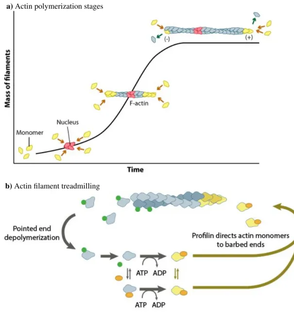
G-actin is a globular protein with a centrally located ATP binding site [67]. If ATP occupies the binding site, multimerization of G-actin monomers occurs, and a helix-shaped polar filamentous polymer called F-actin is formed, see Fig. 1.2a. G-actin attaches to the ATP-binding cleft of another G-actin. Actin filament polymerization oc- curs over three phases [68]: a nucleation phase, an elongation phase, and a steady-state phase. If the G-actin concentration is larger than the critical nucleation concentration, actin nuclei form. In vivo actin nucleation is regulated by proteins [69, 70], which leads to actin nucleation even if the G-actin concentration in the cell is smaller than the criti- cal nucleation concentration. In the elongation phase, free G-actin molecules in the cell attach to actin, generating growing actin filaments. Finally, in the steady-state phase, the actin filament length reaches a constant value. The rate at which the filament polymerizes is equal to the rate of depolymerization.

Actin filaments are polar filaments; actin monomers do not attach or detach from

both ends of the filament at random. G-actin molecules with ATP preferably attach

to the growing end of the filament, the + end. As the filament grows, the ATP starts

to hydrolize to ADP and inorganic orthophosphate, P

. Due to this process, in the

middle of the filament, we find many monomers with ADP-P

. After a while, the Pi

a) Actin polymerization stages

b) Actin filament treadmilling

Figure 1.2: Actin polymerization. a) Nucleation phase, elongation phase and steady-state phase. Figure reproduced from Ref. [49] with permission from MBInfo ©2018 National University of Singapore. b) Actin treadmilling.

Monomers bound to ATP attach to the + end of the filament. Monomers bound

to ADP detach from the - end of the filament. During this process, the fila-

ment length is conserved. Figure reproduced from Ref. [50] with permission from

MBInfo © 2018 National University of Singapore.

1.2 Cytoskeleton

Filament Persistence length Filament length Flexibility

Actin 15 µm 10 µm Semiflexible

Keratin 1 µm 2 µm Semiflexible

Microtubules 6 mm 200 nm - 25 µm Rigid

Table 1.1: Comparison of persistence length and flexibility between the three main types of cytoskeletal filaments of eukaryotic cells. Keratin is a type of intermediate filament. The values in this table are reproduced from the following Refs. [51–53, 84–86].

dissociates from the G-actin molecules. Actin monomers with ADP preferably detach from the shrinking end, the - end. This process leads to constant actin filament length and is know as actin treadmilling [71, 72], see Fig. 1.2b. Under the microscope, a treadmilling actin filament looks like a polymer of constant length, which is being propelled tangentially.

The actin cytoskeleton is essential for mesenchymal motility. At the front of mes- enchymal cells, we find pushing forces due to actin treadmilling. At the cell rear, we find retraction forces caused by actomyosin fibers or myosin-driven actin flow. Here, we focus on the actin polymerization and actin structures at the front of the cell. Actin structures at the rear of the cell are explained in Sec. 1.4.

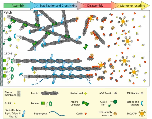
At the front of crawling cells, we typically find two types of actin structures:

branched actin in the lamellipodium, and actin bundles or cables in filopodia, see Fig. 1.3. The most important regulators of the actin assembly machinery in mesenchy- mal cells are the Arp2/3 complex and formins. Actin in the lamellipodium is nucleated by the combined actions of Arp2/3 and its cofactors [74, 75]. In actin bundles actin polymerization is regulated by formins [76].

Actin filaments are formed by polymerizing actin monomers at the barbed end, the + end. Capping proteins can bind to barbed ends, which inhibits further growth and terminates elongation. When an external stimulus triggers a signaling cascade in the cell, the Arp2/3 complex is activated [77, 78]. This protein can initiate new filament branches on preexisting filaments with a characteristic relative angle difference of ∼ 70 ° between both. Another protein that regulates actin dynamics and polymerization in the lamellipodium is cofilin. Cofilin actively severs actin filaments into actin monomers [79].

Formin is a protein which regulates and promotes actin polymerization [80]. Filopodia are tubule-like protrusions at the front of cells, which are made by several actin filaments bundled together. At the tip of filopodia, the concentration of G-actin monomers tends to be lower than in the lamellipodium, and formin is needed to regulate actin polymerization at the tip of filopodia [81, 82]. The depolymerization of actin bundles in the filopodia is also regulated by cofilin. One of the crosslinkers for actin filaments inside bundles is fimbrin.

In cellular processes, the mechanical properties of cytoskeletal filaments are of

course important, in particular, their rigidity, see Fig. 1.4 and Tab 1.1. Filaments

with lengths similar to, or larger than the persistence length, such as actin and in-

termediate filaments, behave as semiflexible polymers. Filaments with lengths much

smaller than the persistence length, such as microtubules, behave as rigid rods.

Figure 1.3: Actin structures in vivo at the front of mesenchymal cells. Top row:

branched actin structure found in the lamellipodium. Bottom row: actin bundles found in filopodia. The left side of the figure represent the cell lipid bilayer, and the right side of the figure indicates the cell inside. Legend with some of the molecules involved in actin polymerization, depolymerization, crosslinking, and capping is shown at the bottom of the figure. Figure reproduced from Ref. [73]

with permission from MBInfo ©2018 National University of Singapore.

1.2 Cytoskeleton

Figure 1.4: Comparison between the shape and dimensions of the three cytoskele-

tal filaments: actin, microtubules, and intermediate filaments. Figure reproduced

from Ref. [83] with permission from the Public Library of Science © 2014 Serge

Mostowy.

Figure 1.5: Myosin motor reaction cycle. In step 1 the myosin head domain attaches to the actin filament in a perpendicular orientation. In step 2 the ADP and Pi are released, and the myosin head changes configuration pulling on the actin. This step is known as the power stroke. In step 3 ATP binds to the myosin head and the head of the motor detaches from the filament. In step 4 the ATP hydrolization occurs and the myosin head recovers the perpendicular orientation with respect to the actin filament. Figure reproduced from Ref. [87] photo credit:

Amazonaws.com.

1.2 Cytoskeleton

1.2.2 Molecular motors

Actin polymerization and nucleation is an ATP-driven process. However, there is also another component of the cytoskeleton that drives the system out-of-equilibrium.

Cytoskeletal motor proteins are a class of molecular motors, composed of a head, a neck, and a tail domain [88], that can move along cytoskeletal filaments [89]. They convert chemical energy into mechanical work by the hydrolysis of ATP. Myosins are associated with actin filaments [88], kinesins [90, 91] and dyneins [92, 93] with microtubules. The interaction between myosin motors and actin filaments are discussed here since these complexes are prevalent in crawling cells.

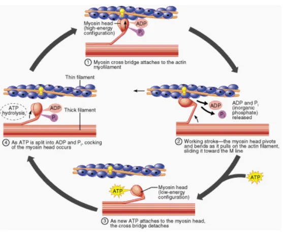
Myosins are a superfamily of molecular motors that comprises several types of myosin motors with different functions. Their heads bind filamentous actin and use ATP hydrolysis to generate force and to ”walk” along the filaments. Their necks act as linkers and as lever arms that translate the forces generated by the motor domains.

Their tails contain the binding sites that determine the specific functions of a particular myosin. The tails of myosins I and V bind to the plasma membrane, that is why these two motors have membrane-related functions [88]. A myosin motor is able to propel actin filaments performing a ”walking cycle” [68, 94]:

• The myosin head domain forms a new bridge to the adjacent actin molecule. A bound ATP molecule hydrolyzes into ADP+Pi, see step 1 of Fig. 1.5.

• The bound actin causes the release of the ADP and Pi molecules, which leads to a conformational change of the myosin head. This acts as a power stroke, see step 2 of Fig. 1.5.

• A new ATP molecule binds to the myosin head which causes the bridge between the actin filament and the myosin head to break, see step 3 of Fig. 1.5.

• Once the ATP molecule hydrolyzes, and the myosin head is in position to bind to the adjacent actin monomer the cycle starts again, see step 4 of Fig. 1.5.

Through this reaction cycle, myosins can take discrete steps along the actin filament.

In in vitro assays, the forces and step size per power stroke of skeletal muscle heavy meromyosin (HMM) are ∼ 4pN and ∼ 11nm, respectively [95]. The most ubiquitous types of myosin are myosin I, II and V. Myosin I is related to vesicle transport [96].

Myosin I has a single head domain and its step size is ∼ 10 nm. Most myosins belong to class II, and they can be found in muscular and non-muscular cells [97]. They consist of two heads, and two tail domains and their step sizes range from ∼ 5 to 15 nm.

Non-muscular myosin II has a fundamental role in processes such as cell adhesion, cell migration, and cell division. Myosin V is a very processive motor. The motor steps follow one another successively since the motor does not often detach [98, 99]. This allows single motors to support the movement of an organelle along its track. Myosin V can move in large steps of ∼ 36nm [100].

1.2.3 Motility assays

Cytoskeletal motility assays are in vitro systems, which were first created to better

understand the interaction between cytoskeletal filaments and molecular motors [101].

a) Motility assay sketch

b) Actin motility assay

c) Microtubule motility assay

Figure 1.6: Cytoskeletal motility assays. a) Molecular motors, HMM, are bound

to a coverslip. After addition of ATP free cytoskeletal filaments, actin, are pro-

pelled by the molecular motors. Figure reproduced from Ref. [4] with permission

from the Nature Publishing Group. b) Actin motility assay with HMM as molec-

ular motors. Snapshots show the filaments collective behavior as the filament

density increases. Figure reproduced from Ref. [4] with permission from the Na-

ture Publishing Group. c) Microtubule motility assay with dynein as molecular

motors. The figure shows snapshots of the same system as time evolves, time

is given in seconds at the top left corner. At the beginning of the experiment,

the microtubules are organized randomly, and at the end of the experiment, the

microtubules are organized in hexagonal-like vortices. Figure reproduced from

Ref. [5] with permission from the Nature Publishing Group.

1.3 Lipid bilayers and plasma membranes

In a motility assay, molecular motors are bound to a functionalized glass surface. Af- ter addition of ATP, free cytoskeletal filaments are moved by the molecular motors over the surface, see Fig. 1.6a. Although apparently a simple system, motility assays give rise to fascinating and complex collective behavior of the cytoskeletal filaments.

Nowadays, motility assays are often studied as model systems for active matter. It is experimentally possible to control the filament and motor concentration, such that motility assays have become an ideal system to develop continuum theories for active matter systems [33, 102, 103].

In actin motility assays with myosin II proteins as molecular motors [4], several phase transitions have been found depending on the filament density, see Fig. 1.6b.

At small actin filament densities, the filaments organize isotropically. As the density increases, the filaments start to show collective behavior. For densities ρ > ρ

, the filaments organize into motile homogeneous clusters. For densities ρ > ρ ∗ > ρ

, actin waves have been observed. In microtubule assays with dynein [5], collective behavior is also observed at large enough densities, see Fig 1.6c. For large densities, the alignment between microtubules leads to self-organization of the microtubules into hexagonal-like vortices. Inside the vortices, the microtubules circulate both clockwise and counter- clockwise. In this experiment, single microtubules are on average ∼ 16 ± 7µm long, whereas the diameters of the vortices are ∼ 400µm. Therefore, the structures observed happen on very large scales and can only be explained by the collective behavior of microtubule bundles.

1.3 Lipid bilayers and plasma membranes

Lipids are amphiphilic molecules that consist of a polar head group and non-polar hydrocarbon tails. The head is hydrophilic, whereas the hydrocarbon tails are hy- drophobic. Because of their amphiphilic nature, lipids adsorb, for instance, at oil-water interfaces. Here, the head group resides in the water, and the hydrocarbon chains point to the oil. Thus, lipids decrease the interfacial tension [104].

Depending on the lipid concentration, several types of self-organized structures in an aqueous solvent can be observed: bilayer, micelle, and liposomes, see Fig. 1.7a. For small lipid concentrations, the entropy dominates over the energy arising from the repul- sion between the hydrophobic tails and the water. As the lipid concentration increases, the minimization of the unfavorable contact between the hydrophobic chains and the water compensates the loss of entropy by micelle formation. The lipid concentration at which micelles are formed is known as critical micelle concentration (CMC) [107].

For even larger lipid concentrations, bilayers and liposomes can be observed.

In monolayers, the lipid type determines the spontaneous curvature. Lipids with

large heads, conical lipids, lead to spontaneous positive curvature. Lipids with large

tails, inverted-conical lipids, lead to spontaneous negative curvature. Cylindrical lipids

lead to planar configurations, see Fig. 1.7b. For lipid bilayers made of one type of

lipids, it is the asymmetry between lipid concentrations in both monolayers that leads

to spontaneous curvature [108]. In cell membranes, the spontaneous curvature is also

related to the asymmetry in the composition between the two monolayers. However,

not only lipids but also proteins can give rise to spontaneous curvature [109].

a) Lipids self-aggregate b) Lipids induce local curvature

Figure 1.7: Lipid bilayers. a) For large enough lipid concentrations lipids ag- gregate in micelles, liposomes and bilayers. Figure reproduced from Ref. [105].

b) Lipids can induce local curvature. Conical lipids induce positive curvature.

Inverted-conical lipids induce negative curvature. Cylindrical lipids do not induce

spontaneous curvature. Figure reproduced from Ref. [106] with permission from

MBInfo ©2018 National University of Singapore.

1.3 Lipid bilayers and plasma membranes

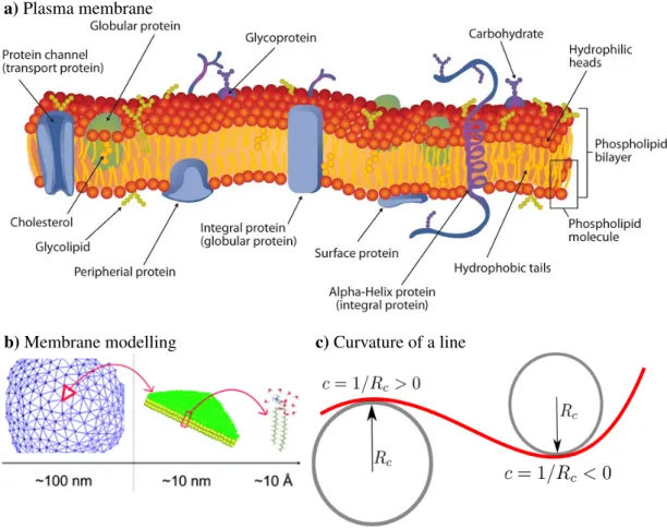
All cells, prokaryotic or eukaryotic, are surrounded by a plasma membrane. This thin and flexible structure acts as the boundary between the interior of the cell and the environment. The plasma membrane is primarily composed of proteins and lipids [110]:

lipids give membranes their flexibility, and proteins assist in the transfer of molecules across the membrane, see Fig. 1.8a.

The three main types of lipids that are found in biological membranes are phospho- lipids, cholesterol, and glycolipids [111]. Phospholipids make up the bulk of the lipids in the cell bilayer. Cholesterols are dispersed between phospholipids, and their role is to modulate plasma membrane permeability, mechanical strength, and biochemical interactions. Glycolipids help the cell to recognize other cells [88].

The cell membrane contains two types of proteins: integral membrane proteins are always inserted into the membrane, whereas peripheral membrane proteins temporarily adhere to the membrane [88, 112]. Membrane proteins fulfill three main functions:

structural proteins are related to cell support and shape, receptor proteins help cells communicate with their environment using signaling molecules, transport proteins and channels are in charge of transporting ions and molecules across the cell membrane.

The plasma membrane is a very complex and heterogeneous system. However, compared to the size of an entire cell, the membrane thickness is negligible. Therefore, on the cell scale, the mechanical properties of the plasma membrane can be modeled using a two-dimensional mathematical surface with curvature-elastic constants, see Fig. 1.8b. For such a continuous description, understanding the concept of curvature is necessary. The curvature of a line is calculated as the inverse of the radius of the circular arc that best approximates the curve at a point, R

, see Fig. 1.8c. To describe a two-dimensional surface, two curvatures at each point are needed. The two principal curvatures, c

, and c

, at a given point of a surface, are the eigenvalues of the curvature tensor at the point.

In 1973, Helfrich proposed a continuum expression for the membrane bending en- ergy [116],

H = 1 2

Z

A

dS

κ(2H + c

)

+ κ

K

. (1.1)

Here, the integral extends over the entire membrane area, κ is the membrane bending rigidity, κ

is the Gaussian splay modulus, H =

(c

+ c

) is the mean curvature, which is calculated as the average of the principal curvatures, c

is the spontaneous curvature, and K = c

c

is the Gaussian curvature, which is calculated as the product of the principal curvatures. If c

6 = 0, there is an asymmetry, such as different lipid and protein concentrations or compositions, between the two monolayers. In such systems, the membrane has a preferred curvature. For simplicity, we only consider cases with c

= 0. The integral of K over a closed surface is associated with the surface topology.

For systems where there are no changes in the global topology, the integral over the

Gaussian curvature is constant, as shown by the Gauss-Bonnet theorem. As such, the

only remaining term relevant for shape changes of the Helfrich bending energy is the

mean curvature H. For coarse-grained simulations of membranes a discretized version

of this model using triangulated surfaces is often employed.

a) Plasma membrane

b) Membrane modelling c) Curvature of a line

Figure 1.8: Modelling the plasma membrane. a) The plasma membrane of eu- karyotic cells is primarily composed of lipids and proteins. The types of lipids found in the plasma membrane are phospholipids, cholesterol, and glycolipids.

According to their structure, the types of proteins found in the surface are in- tegral proteins and peripheral membrane proteins. According to their function, proteins are divided into structural proteins, receptor proteins, and transport proteins. Figure reproduced from Ref [113]. b) On small scales ∼ 10˚ A, the mem- brane needs to be modeled in a very detailed manner using an atomistic approach.

On larger scales ∼ 10nm, the membrane can be modeled using a coarse-grained

approach, e.g., using Martini model [114]. On the cell scale ∼ 100nm, the mem-

brane can be considered as a mathematical surface, which from a computational

point of view is often discretized as a triangulated surface. Figure reproduced

from Ref. [115] with permission from the Royal Society of Chemistry. c) The

curvature of a line is at any point calculated as the inverse of the radius of a

circle with radius R

, which best approximates the curve at that point.

1.3 Lipid bilayers and plasma membranes

a) Sketch cell motility b) Stress fiber types

Figure 1.9: Actin and actomyosin structures in mesenchymal cells. a) Sketch of actin-based cell motility. 1) The cortical cytoskeleton is the portion of the cytoskeleton that lies just beneath the plasma membrane. 2) Focal adhesions are macromolecular assemblies that transmit the forces generated by stress fibers to the substrate. 2b) Transverse arcs are a particular type of stress fibers found at the lamellipodium. 3) The lamellipodium hosts rapid and localized polymeriza- tion of branched actin networks. Initiation of this network occurs via the activity of the Arp2/3 complex. VASP and FMNL2 favor filament elongation, whereas capping proteins block it. 4) Filopodia are filled with parallel actin bundles elongated by VASP and formins and held together by fascin and fimbrin. Fig- ure reproduced from Ref. [117] with permission from the American Physiological Society. b) Stress fibers are contractile actin bundles found in non-muscle cells.

They are made of actin and non-muscle myosin II. Ventral stress fibers are con-

nected by two focal adhesions to the substrate, and they are found at the rear of

the cell. Dorsal stress fibers are connected to the substrate by one focal adhesion,

and the other end is connected to transverse arcs. They are found at the front of

the cell, and they are oriented radially. Transverse arcs are connected to dorsal

stress fibers on both ends. They are found in the lamellipodium, and they are

oriented transversally. Figure reproduced from Ref. [118] with permission from

Rockefeller University Press.

1.4 Cell motility

Cell motility is indispensable for tissue formation during embryogenesis, wound healing and immune response. It is also essential in cancer metastasis, where cancer cells mi- grate from the original tumor towards new locations where metastases are formed [119].

Mesenchymal cell migration is a motility mode based on adhesion. The cells polarize and form a leading edge that extends actin-rich protrusions, leading to adhesive in- teractions with the substrate. Retraction of the contractile cell rear leads to cellular movement. There are two different types of structures in mesenchymal cells: viscoelas- tic actin structures, and elastic, contractile actomyosin structures [117, 120]. Actin structures: lamellipodium, and filopodia exert pushing forces; while actomyosin struc- tures: stress fibers, and myosin-driven actin flow, exert pulling forces. At the front of mesenchymal cells we find the lamellipodium and filopodia, see Fig. 1.9 structures 3 and 4. At the back of the cell, we find myosin-driven actin flow and stress fibers, struc- tures 2a and b. Actin polymerization at the front of the cell both in the lamellipodium and in filopodia is discussed in Sec. 1.2.1.

Stress fibers are contractile actomyosin bundles that have a central role in cell adhesion and morphogenesis. They are composed of bundles of 10 − 30 actin filaments, which are crosslinked together by α-actinin [58]. These actomyosin bundles are typically anchored to focal adhesions, which anchor the actin cytoskeleton to the substrate.

Stress fibers can be divided into three categories:

• Dorsal stress fibers are anchored to focal adhesions at their distal ends. These actin filament bundles do not typically contain myosin II [121]. Although they typically do not exert contractile forces, dorsal stress fibers serve as a platform for the assembly of other types of stress fibers and transmit stresses generated by transverse arcs [118, 121] .

• Transverse arcs are curved actomyosin filament bundles. They do not directly attach to focal adhesions but are connected to dorsal stress fibers. An important feature of transverse arcs in migrating cells is their ability to flow from the leading cell edge towards the cell center [118, 122]. This process is thought to be driven by the continuous contraction of arcs [123].

• Ventral stress fibers, located at the rear of the cell, are contractile actomyosin bundles that are attached to focal adhesions at both ends. They represent one of the major contractile structures in most mesenchymal cells [122].

Keratocytes, keratinocytes, and neutrophils are motile mesenchymal cells. Kerato- cytes are highly specialized corneal stroma cells. The stroma is the part of a tissue or organ with a structural or connective role [124]. The cornea is the outermost layer of the eye. It is the transparent, dome-shaped surface that covers the front of the eye and acts as a lens for the eye. Keratocytes play a crucial role in maintaining the structure and transparency of the cornea. They also play essential roles in corneal wound healing and tissue repair. Keratocytes tend to have fan-liked shapes and are widely used to study mesenchymal cell motility, see Fig. 1.9a. Fast-moving keratocytes with speeds of

∼ 40 µm/s are a classical system to study cell motility. Keratocyte locomotion can also

1.5 Outline of the thesis

a) Actin flow b) Myosin

Figure 1.10: Contractile forces in cell motility. a) Actin flow in a moving kera- tocyte. The myosin-driven actin retrograde flow is strongest at the back of the keratocyte. Figure reproduced from Ref. [129] with permission from Cell Press.

b) Moving keratocyte. Actin is stained in red and myosin is stained in green.

The myosin is mainly located at the back of the keratocyte. Figure reproduced from Ref. [12].

proceed in the absence of front protrusion [125], indicating the existence of an active mechanism independent of actin polymerization. Myosin is found at the rear of ker- atocytes [12, 126], where it contracts the actin network generating a rapid centripetal flow that pulls the rear forward, see Fig. 1.10.

Keratinocytes are the predominant cells in the epidermis [127]. Their primary function is the formation of a barrier against environmental damage by pathogenic bacteria, fungi, parasites, viruses, heat, UV radiation and water loss. Keratinocyte migration plays a crucial role in wound healing. They show elongated half-circular shapes, see Fig. 1.9b. Keratinocytes have a complex network of stress fibers. The flat back of the cells is caused by ventral stress fibers, while the transversal arcs in the lamellipodium help stabilize the half-circular shape.

Neutrophils are the main pathogen-fighting immune cells. Their primary functions are their ability to be recruited to sites of infection, to recognize and phagocytose microbes, and to kill pathogens through a combination of cytotoxic mechanisms. Neu- trophils in bulk adopt spherical shapes, neutrophils on surfaces tend to adopt elongated shapes with a roundish front and a pointed rear, see Fig. 1.9c. Neutrophils perform random motion when there are no external stimuli [128]. However, they show much more directed motion when performing chemotaxis, e.g., chasing bacteria.

1.5 Outline of the thesis

We study the collective behavior of self-propelled rods and present a physical model for cell motility with the use of computational tools and coarse-grained models.

In chapter 2, we present the theoretical background and the model used in our

simulations. A short introduction to the theory and concepts used subsequently is

given. From a simulations point of view, we focus in particular on the model for the

self-propelled rods, the deformable rings, and the rod-ring interactions. In chapter 3,

we describe and analyze the collective behavior and dynamics of density-dependent

a) Keratocyte

c) Neutrophil

b) Keratinocyte

Figure 1.11: Mesenchymal motile cells. a) Movin keratocyte. Arp2/3 is stained

in green and phalloidin is stained in red. Figure reproduced from Ref. [130] with

permission from Rockefeller University Press. Keratocytes typically have fan-like

shapes. b) Moving keratinocyte. Actin is stained in green. Figure courtesy of

Galiya Sakaeva, Dr. Bernd Hoffman, and Prof. Rudolf Merkel. Keratinocytes

show elongated half-circular shapes. c) Neutrophil, in grey, and bacteria, in

yellow. Colored scanning electron micrograph. Neutrophils adhered to surfaces

show elongated shapes with a roundish front and pointed rear. Figure reproduced

from Ref. [131] with permission from Science Photo Library.

1.5 Outline of the thesis

self-propelled rods. The density-dependent mechanism helps the clustering process

and introduces perpendicularity between the rods, which leads to aster formation. In

chapter 4, we describe the different motility patterns showed by complex-self propelled

rings. We model polymerization forces of cytoskeletal filaments by self-propelled rod-

like filaments with constant length pushing against a ring-like confinement. Retraction

forces are modeled by self-propelled rod-like filaments pulling on the confinement. We

correlate the rod dynamics and collective behavior inside the ring with the motion of

the ring. Although the model presented is fairly simple, it still manages to reproduce

cell-like motility patterns. In chapter 5, we extend the complex-ring model by adding

ring deformability. Rod dynamics and alignment now lead to motion and to shape

changes of the rings. We systematically characterize the different shapes obtained

by this model and correlate ring shape and motion. We also study the behavior of

deformable self-propelled rings on walls and at friction interfaces. In chapter 6, we

summarize the results obtained in this thesis, explain the limitations of the models and

give an outlook for future studies.

Chapter 2

Theoretical background, model and simulation techniques

In this section, we briefly present the theoretical background on which our model is based, and the model and simulation techniques used for our systems. Active matter systems, such as motility assays and cells, tend to be surrounded by water. Basic knowledge of fluid dynamics at low Reynolds number is, therefore, necessary to under- stand how such systems move and propel themselves. All the systems studied here are soft matter systems. Soft matter is a subfield of condensed matter, in which systems are deformed or structurally altered by thermal or mechanical stresses of the magnitude of thermal fluctuations. Brownian motion plays a crucial role in the dynamics of the systems studied here.

We focus on two-dimensional simulations because the phenomena we are interested in are mainly two-dimensional. Cytoskeletal motility assays are quasi-two-dimensional systems. The cytoskeletal filaments only escape to the third dimension during crossing events [5]. We simulate cytoskeletal motility assays, gliding bacteria, and self-propelled phoretic particles using self-propelled rods, see chapter 3. Cytoskeletal filaments are linear polymers. Their rigidity is given by the ratio of their contour length l and their persistence length l

. Polymers with l & l

are semiflexible and polymers with l l

are rigid. In cells, actin filaments behave as semiflexible polymers, whereas microtubules behave as rigid polymers [4, 5]. Values for the persistence lengths and typical lengths of cytoskeletal filaments can be found in Sec. 1.2.1. In our simulations, we consider stiff cytoskeletal filament bundles that we model as rods. The activity in our systems is given by the self-propulsion, this is a good approximation for modeling gliding bacteria and motility assays.

The most interesting aspects of mesenchymal cell motility are two-dimensional. The

important effects are the interaction of the cytoskeleton and the lipid bilayer with the

substrate: lamellipodium formation [55], filopodia protrusion [56, 57], and stress fibers

formation [58, 59]. We use quasi-two-dimensional self-propelled rods inside rings to

model cell-like systems, see chapters 4 and 5. In experiments, this would be equivalent

to viewing the section of the cell in contact with the substrate. In our simulations, the

rings act as the cell lipid bilayer. When considering cell motility, the lipid bilayer can

be modeled as a mathematical surface, see Sec. 1.3. Because we only focus on two-

dimensional phenomena for cells attached to planar substrates, we use a semiflexible polymer, instead of the Helfrich Hamiltonian, to model the membrane where it detaches from the substrate.

In the density-dependent rod simulations, rods are initialized inside the simulation box at random positions with random orientations. For the rod-ring simulations, rods are initialized inside the ring with the condition that they cannot cross the ring. This condition holds both for attached and non-attached rods. All rod-rod and rod-ring interactions are calculated using cell lists to minimize computational costs. Also, our code is parallelized using OpenMP.

2.1 Swimming at low Reynolds number

The Navier-Stokes equations were derived by Claude-Louis Navier and George Gabriel Stokes in 1822 [132]. They follow from the conservation and continuity equations, when these are applied to a fluid. For an incompressible fluid, ∇ · v = 0, the Navier-Stokes equations become [133]

ρ ∂v

∂t + (v · ∇ )v

= η ∇

v − ∇ p + f . (2.1) Here, v = v(r, t) is the velocity of a volume element and ∂v/∂t is the acceleration.

(v ·∇ )v is the convective, inertial, or non-linear term and is responsible for the transfer of kinetic energy in the fluid. η ∇

v is the dissipative or viscous term, where η is the fluid viscosity. f = f (r, t) is the external force acting on the volume element. It is possible to make Eq. 2.1 dimensionless by using a characteristic length L and velocity v

Lρv

η

∂v

∂t

+ (v

· ∇ )v

= ∇

v

− ∇ p

+ f

. (2.2) Here, the Reynolds number R = Lρv

/η is a dimensionless quantity that represents the ratio of inertial forces to viscous forces. The fluid behaves very differently at low and at large Reynolds number:

• At low Reynolds number there is no transport of momentum and the fluid re- sponse to forces is instantaneous. The viscous forces are dominant, the flow is laminar, and is characterized by smooth, constant fluid motion.

• At high Reynolds number the motion of a body transfers momentum to the surrounding fluid, which is convected and slowly dissipated. The inertial forces are dominant, the flow is turbulent and is characterized by vortices and other flow instabilities.

For microscopic swimmers, such as E.coli and other cells, R ≈ 10

1 [134]. This means that microscopic organisms swim at low Reynolds number and inertial forces are negligible for microswimmers [135]. For small Reynolds numbers R 1, the Navier- Stokes equation becomes the Stokes or creeping-flow equation

f = ∇ p − η ∇

v. (2.3)

2.2 Langevin equation

Compared with Eq. 2.1, Eq. 2.3 is linear and time-independent. Swimming at low Reynolds number has some unexpected consequences:

• All forces are instantaneously balanced: when a microswimmer propulsion force stops, the swimmer immediately stops. All the momentum transferred to the fluid is instantaneously dissipated.

• Eq. 2.3 is time-independent: the swimmer dynamics must fulfill f (t) = f( − t).

For one-dimensional microswimmers, cyclic motion patterns do not lead to net movement. The forces generated in the first half of the cycle balance the forces in the second half, this is known as the “scallop theorem” [135].

• Microswimmers must have time-irreversible propulsion and a swimming mecha- nism with more than one degree of freedom. In nature, microswimmers developed complicated swimming mechanisms. There are two main swimming mechanisms for microswimmers: waves and reciprocal forces combined with flexibility [136].

2.2 Langevin equation

When studying the dynamics of a particle in a solvent, if the hydrodynamic interactions are screened or can be considered negligible, the surrounding of the particle and its interaction with the solvent can be described in a stochastic manner. An example of this is the Langevin equation

˙

v + γv = f

m + Γ. (2.4)

Here, v is the particle velocity, f is the external force acting on the particle, and Γ is the stochastic force. The interaction between the solvent and the particle is given by γv and Γ, which are the dissipative and stochastic forces, respectively. Typically, the stochastic process is considered Gaussian and Markovian

h Γ(t) i = 0 (2.5)

h Γ(t)Γ(t

) i = aδ(t − t

), (2.6) where a is a measure for the strength of the noise. If we consider a one-dimensional system with m = 1 and no external force, f = 0, the solution of the Langevin equation is

v(t) = v

e

+ Z

0

dt

e

Γ(t

) (2.7)

x(t) = x

+ v

γ 1 − e

+ 1

γ Z

0

dt

1 − e

Γ(t

). (2.8) The velocity autocorrelation function then yields

h v(t)v(t) i = v

e

+ a

2γ 1 − e

−−−→ a

2γ . (2.9)

If we plug the result of the velocity autocorrelation, for t → ∞ , into the equipartition theorem, we obtain the value of the noise autocorrelation function

h E i = k

T

2 = m h v

i

2 = a

2γ . (2.10)

Here, k

is the Boltzmann constant and T is the temperature. With this last result and the noise autocorrelation function we obtain the fluctuation-dissipation theorem [137]

h Γ(t)Γ(t

) i = 2γk

T

m δ(t − t

). (2.11)

The fluctuation-dissipation theorem states: when there is a process that dissipates energy, γv, there is a reverse process related to thermal fluctuations, Γ. The fluctuation- dissipation model holds for all systems which fulfill detailed balance.

The mean squared displacement of the particle in the solvent is given by h (x(t) − x(0))

i = 2γk

T

m t

γ

− 1 − e

γ

. (2.12)

This last equation has two asymptotic behaviors:

• At short times the mean-squared displacement is ballistic

h (x(t) − x(0))

i = h v

i t

. (2.13)

• At long times the mean-squared displacement is diffusive

h (x(t) − x(0))

i = 2Dt. (2.14) Here, D is the diffusion coefficient. The diffusion coefficient can be defined using the mean-squared displacement using the Einstein relation, or from the velocity autocor- relation function using the Green-Kubo relation [137]. Expanding Eq. 2.14 to more dimensions, we obtain

h| r(t) − r(0) |

i = 2dDt, (2.15)

where d is the number of dimensions.

2.3 Anisotropic rod friction

We consider a rod of length L made up of N beads in a fluid [138]. We assume a thin rod that feels a torque M and rotates with angular velocity ω. In the overdamped regime,

ω = M

γ

, (2.16)

where γ

is the rod rotational friction. To calculate γ

, we can estimate the torque created by the friction forces M

upon rod rotation. Since there are no external forces or torques M = ωγ

= − M

. For bead i, the linear velocity v

is

v

= M × idl, (2.17)

2.3 Anisotropic rod friction

where d is the bead diameter and l indicates the direction along the rod axis. The friction force acting on bead i is γ

v

, where γ

is the friction obtained from Stoke’s law. A spherical particle of diameter d in a fluid feels a friction γ

= 3πηd, where η is the fluid viscosity. The friction torque felt by bead i is thus

M

=

N/2

X

i=−N/2

idl × γ

v

= − γ

N/2

X

i=−N/2

i

d

ω = − πL

η

4 ω (2.18)

The rotational friction obtained from this calculation is γ

= πL

η

4 (2.19)

A more precise hydrodynamic calculation, which consists on the derivation of the Smoluchowski equation by the Kirkwood theory for a cylinder gives a correction term α [138]

γ

= πL

η

3 (log (L/d) − α) (2.20)

Using the Einstein relation, we obtain the rod rotational diffusion coefficient D

= k

T

γ

= 3k

T (log (L/d) − α)

πL

η . (2.21)

We now focus on the rod translation. The translational velocity v of the rod can be decomposed in its components, v = v

+ v

, parallel and perpendicular to the long axis of the rod, such that the rod force can be written as

F = γ

v

+ γ

v

, (2.22)

where γ

is the friction coefficient in the parallel direction and γ

is the friction coeffi- cient in the perpendicular direction.

For a system with ”dry” friction, where no hydrodynamic interactions are consid- ered, the parallel and perpendicular frictions are equal, γ

= γ

. Here, each rod bead is considered as a single particle with isotropic friction. Thus, the total rod friction is also isotropic. For a system where there are hydrodynamic interactions, for a rod in a fluid, the rod frictions are anisotropic γ

6 = γ

. We can discretize the rod in Stokeslets, which is the primary Green’s function of the Stokes equation, and integrate the flow that each Stokeslet creates over the rod length. The linearity of the Stokes equation for an incompressible fluid, see Eq. 2.3, means that a Green’s function G exists. The Green’s function is found by solving the Stokes equations with the force term being replaced by a point force acting at the origin and is known as Oseen Tensor

G

(r) = 1 8πηr

δ

+ r

r

r

. (2.23)

Here, the second term of Eq. 2.23 gives rise to the anisotropy in the rod friction.

In our model, we consider a rod embedded in a fluid. This means that although

we perform Brownian dynamics simulations, the rods’ friction coefficients come from

hydrodynamics.

For a rod with a large aspect ratio in a fluid, the parallel and perpendicular friction coefficients, are [133, 138]

γ

= 2πηL

log (L/d) (2.24)

γ

= 2γ

. (2.25)

To obtain the parallel and perpendicular diffusion coefficients we apply the Einstein relations

D

= k

T

γ

= k

T log (L/d)

2πηL (2.26)

D

= k

T γ

= k

T log (L/d)

4πηL . (2.27)

This means that the diffusion in the parallel direction of the rod is two times higher than the diffusion in the perpendicular direction.

2.4 Active Brownian particle model

A spherical active Brownian particle, ABP, is the simplest possible model for a self- propelled particle. An ABP consists of a bead with self-propulsion velocity v

and rotational diffusion D

. The equations of motion of an ABP are

˙

r(t) = v

e(t) + 1

γ

(f(T) + Γ(t)) (2.28)

e(t) = ˙ e(t) × ξ(t). (2.29)

Here, e is the orientation vector of the propulsion force, v

is the propulsion velocity, γ

is the translational friction, f is an external force applied on the particle, Γ is thermal noise associated with the translational motion h Γ

(t)Γ

(t

) i = 2k

T γ

δ

δ(t − t

), and ξ is the noise associated with the rotational motion h ξ

(t)ξ

(t

) i = 2D

δ

δ(t − t

).

The mean-squared displacement of an ABP is given by [18, 139]

h (r(t) − r(0))

i = 4D

t + v

τ

2

2t τ

+ exp( − 2t/τ

) − 1

. (2.30)

Here, r is the ABP position, v

is the ABP self-propulsion velocity, D

is the thermal translation diffusion coefficient for a passive bead, and τ

= 1/D

is the rotational diffusion time of the ABP. Equation 2.30 has three different regimes:

• At short times, t < 4D

/v

, the motion is diffusive, with the thermal translational diffusion coefficient D

h (r(t) − r(0))

i = 4D

t. (2.31)

• At intermediate times, 4D

/v

≤ t ≤ τ

, the motion is ballistic

h (r(t) − r(0))

i = 4D

t + v

t

. (2.32)

2.5 Penetrable self-propelled rods

a) Rod sketch b) Rod potential

0 E r

0 L r

W ( r )

Single bead Along rod axis

Figure 2.1: Rod-rod interaction. a) Sketch of a self-propelled rod. Each rod is discretized into n

beads, F

is the rod propulsion force, v

is the center-of-mass velocity of rod i, ω

is the angular velocity of rod i, r

is the position of the center of mass of rod i, and θ

is the angle that rod i forms with the x-axis. b) Potential profile W (r) along the rod axis, E

is the rod energy barrier. The black curve is the summation of the contributions for all beads of the rod. The rod beads overlap half a bead.

• At long times times, t > τ

, the motion is diffusive with an effective diffusion coefficient D

h (r(t) − r(0))

i = (4D

+ v

τ

)t ≡ 4D

t. (2.33) The diffusion coefficient at large times is always larger than the thermal diffusion coefficient, D

> D

.

The results shown here for the three different regimes apply to an ABP in two dimen- sions.

2.5 Penetrable self-propelled rods

It has been experimentally observed that filaments in motility assays have a finite probability to cross each other [5]. To model such systems in two dimensions, we use an interaction potential that allows crossing events to occur. This means that the potential is finite when two rods overlap.

In our simulations each rod has length L

and is modeled using n

beads to calculate

rod-rod interactions. Rods are characterized by their center-of-mass positions r

, their

orientation angles θ

with respect to the x axis, their center of mass velocities v

,

and their angular velocities ω

[140], see Fig. 2.1a. The rod beads partially overlap,

such that the effective friction for rod-rod interaction is small and no interlocking

occurs [141]. Beads of neighboring rods therefore interact via a separation-shifted Lennard-Jones potential (SSLJ) [140, 142]

W (r) =





 4

σ² α²+r²

−

σ² α²+r²

+ W

r ≤ r

0 r > r

, (2.34)

where r is the distance between two beads, α characterizes the capping of the potential, and W

shifts the potential to avoid a discontinuity at r = r

. The length α = p 2

σ

− r

is calculated by requiring the potential to vanish at the minimum of the SSLJ potential, σ/r

= 2.5, hence the potential is purely repulsive. E

= φ(0) − φ(r

) is the potential energy barrier. Once E

has been set to a certain value, we obtain = α

E

/(α

− 4α

σ

+ 4σ

). With an effective bead radius is r

= r

/2, and an effective rod thickness r

, the rod aspect ratio is a = L/r

. The bead-bead distance within a rod is r

, see Fig. 2.1b.

A system with penetrable self-propelled rods has three energy scales; the thermal energy k

T , the propulsion strength | F

| L

, and the rod energy barrier E

. Two independent dimensionless ratios can be used to characterize the system: the P´eclet number [140]

Pe = Propulsion energy

Thermal energy = | F

| L

k

T = L

v

D

, (2.36)

and the penetrability coefficient [140]

Q = Propulsion energy

Energy barrier = | F

| L

E

. (2.37)

The P´eclet number characterizes the rod activity. If Pe is large, the rod propulsion is high and the effects of the noise are negligible. If Pe is small, the rod propulsion is low compared with the noise. A large Q value indicates that a rod is very penetrable, in such cases crossing events occur often. A small Q value indicates that a rod is impenetrable, in such cases crossing events rarely occur.

The effect of penetrability for self-propelled rods in two dimensions and cytoskele- tal filaments next to surfaces has previously been studied both in simulations and experiments [5, 140], see Fig. 2.2. The rod crossing probability P(φ) can be measured in experiments as a function of the angle between two cytoskeletal filaments φ, see Fig. 2.2b. Because it can also be calculated in simulations initializing two rods close to each other, with well-defined mutual orientations, it allows to connect the parameters in simulations with the experimental data. The simulations performed had different orientation, P´eclet number, energy barrier, and penetrability coefficient, see Fig. 2.2c.

1

In our simulations, we define the P´eclet number using the translational diffusion coefficient.

It is also possible to define the P´eclet number using the rotational diffusion coefficient Pe

= v

D

Lr with Pe = 6Pe

(2.35)

2

In the simulations, a crossing event is counted when two rods intersect significantly, i.e.,

such that the intersection point is at least 0.2L rod away from the ends of each rod. Thus,

events where one rod only “touches” the other rod are not counted.