Very Low Frequency Measurements carried out with an Unmanned Aircraft System

(1)

Very Low Frequency Measurements carried out with an Unmanned Aircraft System

Inaugural-Dissertation zur

Erlangung des Doktorgrades

der Mathematisch-Naturwissenschaftlichen Fakultät der Universität zu Köln

vorgelegt von Rudolf Eröss

aus Köln

(2)

.

Gutachter:

1. Berichterstatter (Betreuer): Prof. Dr. B. Tezkan

2. Berichterstatter: Prof. Dr. A. Junge

Tag der mündlichen Prüfung: 24.06.2015

(3)

.

Abstract

The present thesis, for the first time ever, carries out measurements with the Very Low Frequency (VLF) method with an unmanned helicopter. It is a feasibility study to test the applicability of using the VLF method together with an Un- manned Airborne System (UAS). This sensor-platform combination provides fast data acquisition at low cost. Additionally, a UAS is able to carry out surveys over heavily structured or dangerous terrain at low altitudes. This overcomes limita- tions of ground-based measurements as well as of measurements with manned aircraft.

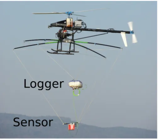
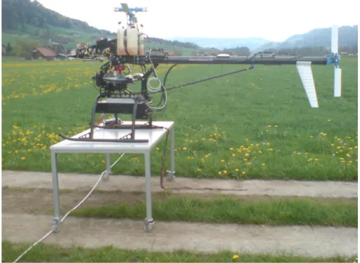
In the geophysical VLF technique, transfer functions relate the vertical magnetic field to the horizontal field components. These transfer functions contain infor- mation about lateral resistivity changes of the subsurface. The presented UAS- VLF measurements are conducted at two sites. As a reference, ground-based VLF and Radiomagnetotellurics (RMT) measurements are carried out addition- ally to the UAS-VLF measurements. Conception and execution of the measure- ments is made in cooperation with Mobile Geophysical Technologies (Celle, Ger- many). The components of the UAS are the unmanned helicopter Scout B1-100 from Aeroscout (Lucerne, Switzerland), the Analogue Digital Unit (ADU) data logger, and the Super High-Frequency induction coil Triple (SHFT) Sensor from metronix.

Achieving meaningful results with this novel sensor-platform combination poses several challenges. No information on how to construct a suitable suspension for the devices was available prior to the present study. On the one hand, the suspension has to minimize interferences such as pendulum motions, gyrations, and electromagnetic noise of the helicopter. On the other hand, it must preserve the airworthiness of the helicopter. For this, measurements of the electromagnetic helicopter noise are carried out and influences of sensor rotations on the transfer functions are investigated. It is shown that small rotations have a large impact on the transfer functions. Furthermore, the ADU data logger must have a distance of 2 m and the SHFT sensor a distance of 4 m to the helicopter. With the help of this information, a suitable suspension was constructed by Aeroscout.

A processing algorithm for the measured UAS-VLF data is developed. Two meth-

ods are presented to determine the transfer functions for available VLF transmit-

(4)

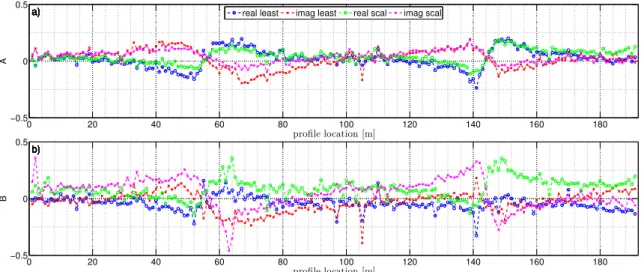
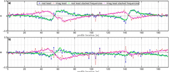
ters in a certain survey area. The transfer functions determined with a bivariate approach are less disturbed than those determined with a scalar approach. A ro- tation of the transfer functions is performed in order to be able to interpret the transfer functions with the 2D inversion algorithm MARE2DEM. In the last step of the processing, the transfer functions are in some cases shifted in order to obtain meaningful inversion models.

The first UAS-VLF field campaign took place in Wavre, Switzerland. The site is characterized by strong anthropogenic anomalies enabling a first proof-of-concept study for the UAS-VLF method. The second field campaign took place in Cux- haven, Germany. This site features a salt- to freshwater transition zone. The transfer functions obtained at the respective sites enable to determine the loca- tions of the anomalies correctly. Furthermore, the transfer functions are used to obtain resistivity models of the subsurface. For this, RMT data provide the back- ground resistivities. This is the first time that resistivity models are determined from UAS-VLF measurements. The inversion models obtained with UAS-VLF data agree well with the ground-based VLF and RMT results. It is shown that forward models explain the measured data well and demonstrate the reliability of the information obtained from UAS-VLF measurements.

ii

(5)

.

Kurzzusammenfassung

In dieser Arbeit werden erstmalig geophysikalischen Very Low Frequency (VLF) Messungen zusammen mit einem unbemannten Hubschrauber durchgeführt. Es ist eine Machbarkeitsstudie, welche untersucht ob es möglich ist die VLF Metho- de mit einem Unmanned Airborne Systems (UAS) zu kombinieren. Diese Kom- bination ermöglicht eine schnelle und kostengünstige Aufnahme von Messdaten.

Darüber hinaus können Daten über schwer zugänglichem oder gefährlichem Ge- lände in geringer Flughöhe aufgenommen werden. Dies umgeht Einschränkungen sowohl von bodengebundenen Messungen, als auch von Messungen mit bemann- ten Flugkörpern.

Bei der VLF Methode stellen Transferfunktionen eine Beziehung zwischen der vertikalen magnetischen Feldkomponente und den horizontalen magnetischen Feld- komponenten her. Diese Transferfunktionen enthalten Informationen über laterale Leitfähigkeitsveränderungen im Erdboden. Für zwei unterschiedliche Messgebie- te werden UAS-VLF Messungen vorgestellt. Als Referenz dienen parallel durch- geführte, bodengebundene VLF und Radiomagnetotellurik (RMT) Messungen.

Die Planung und anschließende Verwirklichung der Messungen wurde in Zusam- menarbeit mit Mobile Geophysical Technologies (Celle, Deutschland) durchge- führt. Die hierfür verwendeten Komponenten des UAS bestehen aus dem unbe- mannten Hubschrauber Scout B1- 100 von Aeroscout (Luzern, Schweiz), dem Analog Digital Unit (ADU) Datenlogger und dem Super High Frequency Indukti- onspulentriple (SHFT) Sensor von metronix.

Um mit dieser neuartigen Sensor-Plattform-Kombination sinnvolle Ergebnisse zu

erhalten, müssen einige Herausforderungen gemeistert werden. Bisher stehen kei-

ne Informationen darüber zur Verfügung, wie eine Aufhängung für die Geräte zu

konstruieren ist. Einerseits muss die Aufhängung den Einfluss etwaiger Störquel-

len auf die Geräte wie etwa Pendelbewegungen und Vibrationen oder elektroma-

gnetischem Rauschen des Hubschraubers minimieren. Andererseits muss Flug-

tauglichkeit des unbemannten Hubschraubers erhalten bleiben. Hierfür werden

Messungen des elektromagnetischen Hubschrauberrauschens durchgeführt und

der Einfluss von Sensorrotationen auf die Übertragungsfunktionen untersucht. Es

wird gezeigt, dass bereits kleine Sensordrehungen großen Einfluss auf die Über-

tragungsfunktionen haben. Außerdem sollte der ADU Datenlogger einen Abstand

(6)

von 2 m und der SHFT Sensor einen Abstand von 4 m zum Hubschrauber haben.

Anhand dieser Vorgaben ist von Aeroscout eine geeignete Aufhängung konstruiert worden.

Für die Auswertung der UAS-VLF Daten wird ein Programmpaket entwickelt.

Zwei Berechnungsmethoden werden vorgestellt, welche die Transferfunktionen aus den in einem gegebenen Messgebiet vorhandenen VLF Sendern bestimmen.

Auf Übertragungsfunktionen die mit der bivariaten Methode berechnet werden, haben Störungen weniger Einfluss als Übertragungsfunktionen die mit der skala- ren Methode berechnet werden. Die berechneten Übertragungsfunktionen werden rotiert um eine Interpretation mit dem MARE2DEM 2D-Inversionsalgorithmus zu ermöglichen. Im letzten Schritt der Datenverarbeitung werden Verschiebungen der Übertragungsfunktionen korrigiert. Dies ist teilweise notwendig um aussage- kräftige Inversionsmodelle zu erhalten.

Das erste Gebiet, in welchem UAS-VLF Messungen realisiert wurden, liegt in Wavre in der Schweiz. Hier wird zunächst erprobt ob und wie gut anthropoge- ne Anomalien mit der UAS-VLF Methode detektiert werden können. Das zwei- te Messgebiet liegt bei Cuxhaven in Deutschland über einem Salz- zu Süßwas- serübergang. Die jeweils berechneten Übertragungsfunktionen ermöglichen es, die Position der Anomalien im Untergrund korrekt zu lokalisieren. Die Übertra- gungsfunktionen können außerdem dazu verwendet werden Leitfähigkeitsmodel- le des Untergrunds zu erhalten. Hierfür werden die RMT Daten zur Bestimmung der Hintergrundleitfähigkeiten verwendet. Dies ist das erste mal, dass Leitfähig- keitsmodelle aus gemessenen UAS-VLF Daten abgeleitet werden. Die mit der UAS-VLF Methode bestimmten Positionen der Anomalien im Untergrund stim- men mit den Positionen, welche mit bodengebundenen VLF und RMT Messungen bestimmt wurden, überein. Es wird gezeigt, dass Vorwärtsmodellierungen in der Lage sind die gemessenen UAS-VLF Daten zu erklären und dass sie die Verläss- lichkeit der gewonnen Informationen bestätigen.

iv

(7)

.

Abbreviations

ADU Analog/Digital Signal Conditioning Unit-07

ASCII American Standard Code for Information Interchange

dB decibel

GPS Global Positioning System

ICAO International Civil Aviation Organization

MB megabyte

RPA Remotely Piloted Aircraft

ROV Remote Operated Vehicles

SHFT Super High-Frequency induction coil Triple SI International System of Units

UA Unmanned Aircraft

UAS Unmanned Aircraft System

UAV Unmanned Aerial Vehicle

USB Universal Serial Bus

RMT Radiomagnetotellurics

VLF Very Low Frequency

(10)

(11)

.

1 Introduction

1.1 Motivation and Objectives

The major aim of the present thesis is to answer the question whether it is possible to con- duct measurements with the geophysical Very Low Frequency (VLF) method on board of an unmanned aircraft and receive meaningful data. Why should one try to do such a thing, as ground-based measurements and manned aircraft measurements with the VLF method already exist and are well established (e. g. Pedersen et al. [1994]; Bosch and Müller [2005])?

The reason is that measurements on board of an unmanned aircraft have several advantages compared to ground-based measurements. Firstly, an unmanned aircraft can measure over heavily structured or even impassable terrain. It can fly autonomously with a constant veloc- ity over pre-defined profiles, thereby measuring on a regular grid with straight profile lines [Clarke, 2014]. The velocity of an unmanned aircraft can be adapted to the type of geophys- ical problem investigated. In general, a measurement conducted with an unmanned aircraft covers a greater area in the same time than a ground-based measurement.

In comparison to a manned aircraft, an unmanned aircraft can fly at very low altitudes down to a couple of meters above ground (e. g. Tezkan et al. [2011]). Additionally, unmanned aircraft are able to fly with very slow velocities – especially compared to manned aeroplanes.

This enables measurements with a higher accuracy and helps to find even small geophysical anomalies since the electromagnetic fields originating from subsurface anomalies decay with increasing altitude [Pedersen and Oskooi, 2004]. The listed advantages make geophysical measurements on board unmanned aircraft valuable for medium sized survey areas, that is several profiles with profile lengths of several hundred meters.

Several steps need to be taken to enable measurements with the geophysical VLF method combined with an unmanned aircraft and receive meaningful and interpretable data sets. The most important step is to realize a flight. To tackle this hurdle, an appropriate suspension which preserves a stable and safe flight and simultaneously enables low noise environment for the sensor, which is mounted as low as possible, is needed. A logger and a sensor implemented in inappropriate way may result in a perilous double pendulum – endangering safe flight.

The next step is to find survey areas that are adequate for first UAS-VLF measurements. A

suitable survey area should contain subsurface anomalies that are detectable under the difficult

(12)

conditions which a proof-of-concept study poses. For the first measurement campaign, an area with two anthropogenic anomalies is chosen. Here, the system is tested above relatively easy to detect subsurface anomalies. For the second measurement campaign, an area with a more natural target is chosen. It is investigated whether the UAS-VLF method is able to detect a salt- to freshwater transition zone. In both survey areas, ground-based VLF and RMT measurements are carried out firstly as a reference for comparison with the results of the UAS- VLF and secondly also to obtain the background resistivities of the survey areas.

Another important step is an adequate data processing, considering that the sensor is in a certain altitude above ground. First, an appropriate time series processing is performed and a method to identify the used transmitters is defined. Second, a method to determine the transfer functions (scalar or bivariate) is developed – including filtering and other corrections of the resulting transfer functions. Third, a quantitative interpretation of the data using the derived subsurface resistivity models is conducted.

The following questions are addressed in the present thesis:

• Is it possible to perform VLF measurements with an unmanned aircraft and obtain mean- ingful data?

• What additional problems occur during data processing if data of an UAS is used?

• How can crucial problems – like gyrations of the sensor and airworthiness of the UAS – be solved and how can the received data be processed appropriately?

• Are the subsurface anomalies detectable?

• Is it possible to obtain meaningful resistivity models of the subsurface from the UAS- VLF data?

• Are the obtained UAS-VLF results comparable with ground-based results?

• Do the obtained results agree with results of other geophysical methods?

1.2 Overview

This study is organized as follows. An introductory overview of basic electromagnetic con- cepts is given in Chapter 2. After this, the concept behind the geophysical methods (VLF and RMT) applied in the present work is explained. For the VLF method, a scalar and a bivariate approach to determine the Tipper is presented. The final sections of Chapter 2 are dedicated to explain the applied modelling and inversion theory. In Chapter 3, the terminol- ogy of unmanned aircraft is discussed and the UAS and the applied devices are introduced.

Subsequently, the processing of the VLF data is explained step by step in Chapter 4. The first three sections describe the data acquisition method, the time series analysis and how VLF

2

(13)

transmitters are identified. Afterwards, in sections four and five, it is described how the de- termination of the transfer functions is performed for the scalar and for the bivariate approach and the results are verified. The last sections of Chapter 4 describe additional adjustments to the transfer functions. Chapter 5 describes preparative experiments regarding helicopter noise and rotations of the sensor. It draws conclusions for the special suspension that needed to be constructed to enable the UAS-VLF measurements. An overview of the survey areas of the two measuring campaigns is given in Chapter 6. Chapter 6, additionally, presents the modelling and inversion results of the RMT and VLF data of the two measuring campaigns.

Finally, in Chapter 7, results of the present work are summarized and suggestions for further

research is given in Chapter 8.

(14)

(15)

.

2 Theory

The present chapter first gives an introduction into the basics of the electromagnetic theory.

Then, the Very Low Frequency (VLF) method is introduced. The possibilities, advantages, and disadvantages of the VLF method regarding geophysical problems are discussed. Sub- sequently, a description of the Radiomagnetotellurics (RMT) method is presented. At the end of this chapter, the theory underlying the applied modelling and inversion algorithms is explained. Following this general overview, the applied algorithms are described.

2.1 Electromagnetic Theory

Geophysical induction methods are most commonly applied with the goal of determining the electrical resistivities ρ (or electrical conductivities σ = 1/ρ) of the subsurface. The resistivi- ties ρ of the subsurface vary in many orders of magnitude depending on the properties of the materials in the ground.

In general, clays have different resistivities than rocks. In addition, the resistivities depend on the water saturation of the subsurface material and the salinity of the saturating water also plays an important role for the resistivities. Generally, matter with more free electrons has a lower resistivity than matter with less free electrons [Telford et al., 1990].

The equations that describe the interaction of electromagnetic fields with matter are Maxwell’s equations. The Maxwell’s equations consist of four coupled first order linear differential equa- tions. They can be written in differential or integral form:

∇· D = q

Z

S

D· dS = Z

V

q· dV (1)

∇· B = 0

Z

S

B· dS = 0 (2)

∇ × H = ∂D

∂ t + j

I

l

H· dl = Z

S

j + ∂D

∂ t

· dS (3)

∇ × E = − ∂B

∂t

I

l

E· dl = − Z

S

∂B

∂t · dS (4)

(16)

The variables are specified in Table 1. Using Gauss’ and Stocks’ theorem, Maxwell’s equa- tions can be derived in their integral form [Jackson, 1975]. Gauss’s law (equation (1)) de- scribes the relationship between the electrical field D and the electric charges q that cause it.

Equation (2) states that magnetic fields B are source free, it is called Gauss’s law for mag- netic fields. Ampère’s law (equation (3)) states that fields can be generated in two ways, by line currents j and displacement currents

^∂D_∂t

. Equation (4), Faraday’s law, states that a vary- ing magnetic field B causes an electric field E of opposite sign. Of superior importance for geophysical electromagnetic induction methods are equations (3) and (4).

Table 1: Variables and constants used in electrodynamics. Vectors written in bold. Dimensions of the quantities are given in the International System of Units (SI).

Parameter Symbol SI Unit

electric field intensity E

^V_m

electric displacement field (flux density) D

_m^As2

magnetic field (flux density) B T =

_m^Vs2

magnetic field intensity H

^A_m

current density j

_m^A2

electrical permittivity =

₀

_r _Vm^As

electrical permittivity of free space

₀

= 8.845 · 10

⁻¹² _Vm^As

relative electrical permittivity

_r

non-dimensional

magnetic permeability µ = µ

₀

µ

_r _Am^Vs

permeability of free space µ

₀

= 4π · 10

⁻⁷ _Am^Vs

relative permeability µ

r

non-dimensional

electrical conductivity σ

_Vm^A

electrical resistivity ρ Ωm =

^Vm_A

angular frequency ω = 2πf

¹_s

frequency f

¹_s

The relation to subsurface matter, which is the target in applied geophysics, is given by Ohm’s law:

j = σE (5)

The so called constitutive equations,

B = µH D = εE (6)

6

(17)

describe firstly the relationship between the electric field intensity E and the electric displace- ment field D, and secondly between the magnetic field B and the magnetic field intensity H in media. However, they reduce to scalar quantities in isotropic media. For most subsurface materials, the magnetic permeability µ equals the vacuum permeability µ

0

. These assumptions are often made in the applied geophysics and are applied in the present thesis.

From the material equations (5) and (6), the telegraph and Helmholtz equations can be derived.

These describe the damped propagation of electromagnetic fields. With the two assumptions that outside external sources and in regions of homogeneous conductivity, no free charges exist, and the current density is source free in homogeneous regions, ∇· E = 0 and ∇· j = 0.

With these simplifications, and by taking the curl of Faraday’s law and substituting ∇ × B with Ampère’s law, the telegraph equation is:

∆F = µσ ∂

∂t F + µε ∂

²

∂

²

t F F ∈ {E, H} (7)

The derived equation for H is identical. The first term on the right contains the conductivity and describes diffusion whereas the second term describes the wave propagation of the field.

By Fourier transformation, the wave equation can be transformed into the frequency domain resulting in the Helmholtz equation (with ∂

_t

= iω),

∆F = iωµσF + µεω

²

F F ∈ {E, H} (8)

with the wavenumber k, which implies the physical properties of media as k

²

= µεω

²

− iµσω.

The quasi static approximation (µεω

²

µσω) is commonly applied to equation (7) and (8) and simplifies them to:

∆F = µσ ∂

∂t F F ∈ {E, H} (9)

∆F = iωµσF F ∈ {E, H} (10)

This approximation is valid if conducting currents (σE) are much larger than displacement currents (∂

t

D). However, in high resistivity environments (e. g. an air layer) and high op- erating frequencies, the validity of the approximation is questionable (e. g. for UAS-VLF modelling).

For a homogeneous half-space equation (10) reduces to:

∂

²

F

∂z

²

= iωµσF = k

²

F F ∈ {E, H} (11)

and its general solution,

F = F

₀

e

^−ik

+ F

₁

e

^+ik

(12)

(18)

simplifies to F

₀

e

^−ik

describing an exponential decay with depth z. With the electric field given by E=E

_x

e

^−ik

and the magnetic field given by B=B

_y

e

^−ik

with E

_x

and B

_y

interrelated through Faraday’s law (equation (4)) follows:

∂E

x

∂z = −E

_x0

ke

^−kz

= −iωB

_y

= −iωB

_y0

e

^−kz

(13) The so called magnetotelluric impedance is then given by the relation of the electric and the magnetic field [Brasse, 2007]:

Z(ω) = E

x0

B

_y0

= iω

k = iω

√ iωµσ = s

iω

µσ (14)

Maxwell’s equations (3) and (4) yield to two decoupled sets of equations. With ∂

_x

≡ 0 and assuming time dependence e

^iωt

they become,

∂

_y

B

_z

− ∂

_z

B

_y

= µ

₀

(σE

_x

+ j

_x

) ∂

_z

E

_x

= −iωB

_y

−∂

_y

E

_x

= −iωB

_z

(15)

∂

_y

E

_z

− ∂

_z

E

_y

= iωB

_x

∂

_z

B

_x

= µ

₀

(σE

_y

+ j

_y

) −∂

_y

B

_x

= µ

₀

(σE

_z

+ j

_z

) (16) The first set of equations (i. e. (15)), in which the strike direction is parallel to the E-field, is called transverse electric (TE)-mode or E-polarization. The complementary second set of equations (i.e. (16)), in which the strike direction is parallel to the B-field, is called transverse magnetic (TM)-mode or B-polarization [Chave and Jones, 2012]. Strike directions for two dimensional models characterize the direction along which a conductivity structure is constant.

The depth where the absolute value of an electromagnetic wave of frequency f has decayed to 1/e is defined as skin or penetration depth δ:

δ = r 2

µωσ (17)

With µ = µ

₀

, ω = 2π/T and ρ = 1/σ equation (17) becomes an approximation for the skin depth:

δ ≈ 500 p

ρ/f [m] (18)

Thus, the skin depth is a function of resistivity and frequency.

Another method to determine the depth of investigation is to consider the phase φ information of the subsurface, which leads to the equation for z∗:

z

^∗

= r ρ

ωµ sin(φ) (19)

8

(19)

For details on electromagnetic theory it is referred to Jackson [1975], or with a relation to geophysics Telford et al. [1990].

2.2 Very Low Frequency Method

Here, at first, the physical concept behind the VLF method is explained. Subsequently, the methods to calculate the transfer functions are described.

2.2.1 Concept of the Method

The geophysical VLF method is a passive electromagnetic method. It exploits existing radio transmitters (usually used for communication with submarines). VLF transmitters are dis- tributed globally. They use the frequency range of 15 kHz to 30 kHz, the so called VLF band.

The possibility to use VLF transmitters to investigate the subsurface was described first by Paal [1965]. Since then, the VLF method is widely used as a near-surface geological mapping tool. An advantage of the VLF method is that there is no need to set up transmitters in the field. This makes measurements easier regarding logistical effort and cheaper compared to methods that need transmitters in the field. The depth of investigation for the available VLF frequencies usually ranges from several meters to 100 m, depending on the resistivity distribu- tion of the subsurface. Since VLF is based on electromagnetic induction, it is sensitive to good conductors. The reason is that in good conductors the current density becomes stronger. One major disadvantage is that it is not possible to derive any direct quantitative information on the electrical properties of the subsurface with the VLF method, it is only possible to detect lateral conductivity changes. To derive a subsurface resistivity distribution is usually the main goal and advantage of geophysical electromagnetic methods. However, VLF is an effective map- ping method, large areas can be investigated in a very time efficient way compared to other electromagnetic methods, because the sensor does not require direct contact to the surface.

Another disadvantage of the VLF method is the dependency on signals of remote transmitters, that is their existence and quality in terms of signal to noise, in a certain measuring area. The sensitivity of the VLF method to anthropogenic noise sources, such as high voltage power lines or railway lines, can also impede the quality of measured data.

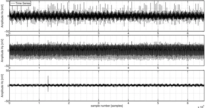
For measurements conducted with the geophysical VLF method, it is necessary to record the vertical magnetic field component H

z

and at least one of the horizontal magnetic field components H

_x

or H

_y

. Usually, the magnetic fields are measured along a profile. The recorded fields are a combination of the primary fields of VLF transmitters and the secondary fields (induced by the primary fields of VLF transmitters).

The vertical magnetic field component H

z

is only present over or in the vicinity of lateral con-

ductivity changes in the subsurface. The primary horizontal magnetic field (created by remote

VLF transmitters) induces eddy currents in conductive bodies in the subsurface. These eddy

(20)

currents create the secondary vertical magnetic field H

_z

that is essential for the VLF method.

In areas without lateral conductivity changes, the H

_z

component is zero. In other words, the VLF method is able to detect lateral conductivity changes in the subsurface (cf. Figure 1).

Vozoff [1972] assumes that the vertical component of the magnetic field H

z

is linearly related to the horizontal components H

_x

and H

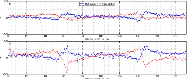
_y

, resulting in the following relationship:

H

_z

(ω) = A(ω) · H

_x

(ω) + B(ω) · H

_y

(ω) (20) This linear relation – the transfer function – between the horizontal and the vertical magnetic field (A, B) is also called the Tipper vector where, ω is the angular frequency and (H

x

, H

y

, H

_z

)

^T

is the complex magnetic field vector [Pedersen et al., 1994].

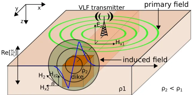
Figure 1: Sketch of the VLF method. The primary magnetic field H

_x1

(green lines), generated by a VLF transmitter, induces eddy currents in a conductive subsurface body. These currents create the secondary magnetic field components H

x2

and H

z2

(shaded circles).

The blue line shows the real part of the magnetic transfer function (or tipper) B, that is Re(H

z

/H

x

) = Re(B), along a profile at a selected VLF frequency [Bosch and Müller, 2005; Eröss et al., 2013].

As stated above, the VLF method is only sensitive for lateral conductivity changes. For a layered Earth (one dimensional case), both components of the Tipper vector equal zero. In a two dimensional case, the occurrence of the vertical magnetic field component H

_z

is utilized.

In case of a linear, lateral conductivity change exactly parallel to one of the axes of a chosen coordinate system (geological strike axis), the corresponding Tipper component (orthogonal to

10

(21)

the profile) is zero and the other one is not zero (2D case). That is, if the strike of an anomaly is parallel to the y-axis, the B component of the Tipper equals zero and the A component differs from zero.

The common case in the field is that neither A nor B equal zero. This either indicates a three dimensional anomaly or that the strike of the anomaly is not orthogonal to the chosen profile direction, resulting in a contribution to both Tipper components [Vozoff, 1972].

2.2.2 Calculation of the Tipper

In general, one can distinguish between two methods to calculate the tipper: the scalar and the bivariate approach. Both are briefly introduced in the following.

For the scalar approach, it is assumed that the subsurface anomaly (i. e. a good conducting body) is 2D and that one of the axes of the coordinate system is parallel to the anomaly. As a result, one component of the Tipper equals zero [Vozoff, 1972]. In the case of a strike exactly parallel to the y-axis (B = 0), equation (20) simplifies to

H

_z

(ω) = A(ω) · H

_x

(ω) (21)

considering H

_z

as noise free and the A component of the Tipper can simply be calculated as H

_z

(ω)

H

_x

(ω) = A(ω) (22)

and vice versa for the B component (after [Pedersen and Oskooi, 2004]). However, Pedersen et al. [1994] describe as a drawback that determining the transfer functions out of a single frequency can bias the result, emphasizing anomalies aligned with the direction of the used transmitter.

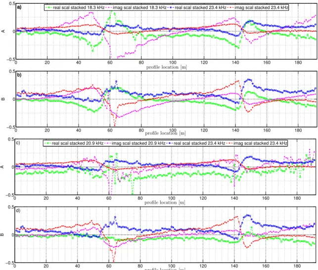
The bivariate approach is more complex, but has some advantages. It exploits the fact that often more than one transmitter is available at a certain measuring site and at a certain time.

Ideally, the Tipper vector is calculated with two independent measurements at the same angu- lar frequency ω but different transmitter directions (ideally 90

^◦

). In reality this is not possible because every transmitter uses a unique frequency and the transmitters are distributed irregu- larly. Therefore, it is assumed that the Tipper is independent of frequency in the VLF band.

In this case, the Tipper can be calculated by all received transmitters or a number of chosen transmitters. Using all the information the different transmitters provide at once leads to a more stable Tipper vector with increasing number of frequencies [Pedersen et al., 1994]. The Tipper vector is calculated via a least squares approach (gennerally explained in e.g. Chave and Jones [2012])

T = (G

^T

· G)

⁻¹

· G

^T

· d (23)

(22)

with the Tipper vector T(ω)

T(ω) = (A(ω), B (ω))

^T

(24) and the M × N matrix G(ω) containing the horizontal components H

_x

and H

_y

of the magnetic field,

G = (H

x

(ω

i

), H

y

(ω

i

)) (25) and d(ω) = H

z

(ω

i

) the vector containing the vertical magnetic field component H

z

at certain frequencies. ω

_i

indicates the different transmitter frequencies. For example, if only three transmitters are used, G is a matrix of dimension 3 × 2 [Hansen et al., 2012].

It is notable that the least squares problem can only be solved if the inverse (G

^T

· G)

⁻¹

exists, which requires det(G

^T

· G)

⁻¹

6= 0. This is the case if transmitters for two or more directions are available. For exact two transmitters of different directions, the least squares solution is exact because in this case equation (23) is a set of two equations and two variables. For transmitters of three or more directions, the solution is a least squares approximation. If all transmitters are in one direction, no additional information is gained and det(G

^T

· G)

⁻¹

can become zero. The reason is that two (linearly) independent realizations are required to find the transfer functions [Hansen et al., 2012].

2.3 Radiomagnetotellurics Method

Figure 2 shows the principle of the Radiomagnetotellurics (RMT) method. Horizontal mag- netic and electric fields are measured orthogonal to each other. With the usage of transmitters of different frequencies, a broader range of depths can be investigated compared to VLF. This way, information of the subsurface resistivity distribution is gained. The quantities derived from the measured magnetic and electrical fields are the apparent resistivity ρ

_a

and the phase φ.

Like the VLF method, the RMT method uses radio transmitters, that is no transmitter is needs to be applied in the field. However, the used frequencies are in range from 10 kHz to 1 MHz.

Therefore, RMT is a method to investigate depths from few meters up to 100 m and strongly dependent on the resistivity distribution of the subsurface. Similar to VLF, RMT is an induc- tion method and sensitive to good conductors since the induced current densities are stronger in good conductors. Electric fields are measured with grounded electrodes and magnetic fields are measured with inductions coils. The big advantage of the RMT method compared to VLF is the possibility to derive a resistivity model – and thus quantitative information – of the sub- surface. As for VLF, disadvantages of the RMT method are the dependency of the quality on foreign transmitter signals and the sensitivity to anthropogenic noise sources such as high voltage power lines or railway lines.

The theory to calculate apparent resistivity ρ

_a

and phase φ is similar to the magnetotelluric

12

(23)

(MT) theory [Cagniard, 1953]. The complex impedance tensor Z specifies the ratio between the measured electric and magnetic fields (Equation 26).

E

_x

(ω) E

y

(ω)

=

Z

_xx

Z

_xy

Z

yx

Z

yy

H

_x

(ω) H

y

(ω)

(26)

Figure 2: Sketch of the RMT method. The magnetic field H

_y

generated by a radio transmitter (modi- fied after Recher [2002]).

For a 2D resistivity distribution, two modes can be distinguished. The tangential electric, with the strike of the anomaly parallel to the transmitter direction, and the tangential magnetic, with the strike of the anomaly orthogonal to the transmitter direction. The apparent resistivities ρ

_a

and phases φ for both modes are calculated as follows:

ρ

_a_ij

= 1

ωµ |Z

_ij

(ω)|

²

(27)

φ

_ij

(ω) = arctan

imag(Z

_ij

) real(Z

_ij

)

, with i, j ∈ x, y, i 6= j (28)

where µ is the magnetic permeability and ω the angular frequency [Recher, 2002].

(24)

2.4 Modelling and Inversion

Measured geophysical field data can usually be used to compute resistivity models of the subsurface, which is the goal of electromagnetic geophysical methods. The search for a re- sistivity model that explains the measured data well including possible a priori information, is commonly termed inversion. In contrast, the process of computing synthetic data from a constructed resistivity model, is called forward modelling (the obtained data is synthetic since it stems from an artificial model and is not measured). For the inversion process, measured and synthetic data are compared and if they differ (by a certain defined level), the resistivity distribution of the subsurface model is changed (model update) and repeatedly compared with the measured data. This process can be iterated until measured and synthetic data agree to a satisfactory degree. For example, if their deviation falls below a certain defined level. Of- ten experience and time is needed to achieve meaningful models in this way. Since manual model updates are very time consuming even for simple subsurface resistivity distributions, the inversion process can be automated (cf. Figure 3).

Figure 3: Sketch of the inversion process [Recher, 2002].

Therefore, the inversion uses an iterative scheme – changing the model parameters m of the subsurface model – to fit the observed data d. The goal is to match measured and synthetic data within a predefined error range [Recher, 2002]. The inversion is repeated iteratively and the model parameters m

_k

are updated until the predefined goal is achieved or no further improvement is possible:

m

k+1

= m

k

+ ∆m

k

(29)

2.4.1 Inverse Problem

As stated above, the goal of an inversion is to find a resistivity model that explains the (VLF or RMT) data d

_i

, i = 1, ..., N , which contains the measured information. N is the number of measured data. For this, a parametrization of the subsurface represented by the model parameters m

i

, i = 1, ..., M , is needed. For a more concise notation, the m

j

can be considered as components of an M -dimensional column vector m

m = (m

₁

, m

₂

, ..., m

_M

)

^T

(30)

14

(25)

and the observed data d of components of the N-dimensional column vector [Chave and Jones, 2012]:

d = (d

₁

, d

₂

, ..., d

_N

)

^T

(31) For an inversion it is necessary to have a so called forward algorithm. This algorithm enables to calculate the synthetic data that would be observed with a given model parametrization.

This part of the inversion is called forward problem (equation (32)). The forward calculation derives electromagnetic fields out of geophysical quantities, that is the model parameters that form a resistivity distribution of the subsurface – strait forward – to emphasize: in this part no inversion takes place. In the best case, the measured data d would equal the forward calculation of the model m,

d = f (m) = (f

₁

(m), f

₂

(m), ..., f

_N

(m))

^T

, with i = 1, 2, ..., N (32) which is the transformation from model to data space. Here, the functions f

i

are implicitily de- fined by a code that solves the Maxwell equation. The solution is converted to the appropriate quantity defineing d

_i

[Chave and Jones, 2012].

Forward Problem

If the physical parameters of the Earth are independent of one Cartesian coordinate (2D case), Rodi and Mackie [2001] show that Maxwell’s equations can be decoupled in the transverse electric and transverse magnetic polarization. The source of the electromagnetic fields can be modelled as a current sheet at a height z = −h. In the quasi static approximation, to calculate RMT data [Schmucker and Weidelt, 1975], it is enough to solve,

∂

²

E

_x

∂y

²

+ ∂

²

E

_x

∂z

²

= −iωµσE

_x

(33)

∂E

_x

∂z

_z=−h

= iωµ (34)

for the TE-mode with E

_x

in strike direction and

∂

∂y

ρ ∂H

x

∂y

+ ∂

∂z

ρ ∂H

x

∂z

= −iωµH

_x

(35)

H

_x

z=0

= 1 (36)

for the TM-mode with E

_x

orthogonal to strike direction (cf. Section 2.1), where µ is the mag-

netic permeability and ω the angular frequency. The apparent resistivity of the TE polarization

(26)

after equation (26) is defined as ρ

a

= 1

ωµ (Z

xy

) = 1 ωµ

E

_x

H

_y

[Ωm] (37)

with H

_y

implied from Maxwell’s equations as H

_y

= 1

ωµ

∂E

_x

∂z (38)

For the TM polarization it is ρ

_a

= 1

ωµ (Z

_yx

) = 1 ωµ

E

_y

H

_x

[Ωm] (39)

and

E

y

= ρ ∂H

x

∂z (40)

Here, the model parameters (resistivities and thicknesses) and the angular frequency are the input parameters of the forward calculation. The forward code calculates the apparent resis- tivities ρ

_a

and phases φ for given frequencies ω and for a given resistivity model.

However, a model (of discrete parameters) is commonly not able to reproduce measured and thus noisy data. Considering errors in the prediction, data and model parameters of a subsur- face model are related in the following way:

d

_i

= f

_i

(m

₁

, m

₂

, ..., m

_M

) + e

_i

, with i = 1, 2, ..., N (41) With these considerations and assuming the inverse of f exists (and e = 0), it is easy to see where the term inversion comes from, since the solution of the linear case of equation (41) is

m = f

⁻¹

(d) (42) In other words, solving equation (41) equals finding the inverse of f , which is f

⁻¹

[Chave and Jones, 2012].

However, for most problems investigated in geophysical context, the inverse of f does not exist. Therefore, the goal is to find an estimate of the model m to explain the measured data d in the best way. If the data noise is uncorrelated and normally distributed, this can be achieved by a least-squares approach [Chave and Jones, 2012].

16

(27)

2.4.2 Least Squares Solution

Geophysical problems for which the number of unknown model parameters is smaller than the number of data points (M < N ) are stated over-determined problems. For this kind of over-determined problems, it is possible to use the least squares method to match the measured data as closely as possible or in a predefined way (e. g. RMS), but not exactly. In geophysics, this means to minimize the data misfit or objective function Φ

_d

(m), that is the discrepancy between d and the forward functional f(m)=Gm [Chave and Jones, 2012]

Φ

d

(m) = (d − Gm)

^T

(d − Gm) (43) Minimization of Φ

_d

(m) requires

^∂Φ(m)_∂m

i

=0. Calculating the derivative of Φ

_d

(m) with respect to m leads to

G

^T

Gm − G

^T

d = 0 (44) If the inverse of G

^T

G exists, the model vector is received by the data vector for this uncon- strained least square approach. Solving for m results in the normal equation:

m = (G

^T

G)

⁻¹

G

^T

d (45) 2.4.3 Linearization

In geophysics, the relation between m and d is often not linear. That is the earth response f(m) is not linear with the change of the physical properties m. However, it is assumed that linear behaviour for very small changes of the properties. In this case, the forward function f(m) can be linearized. The linearization is accomplished by expanding f (m) in a Taylor series around a known model m

₀

. Then equation (41) can be written as

d = f(m) = f(m

₀

) + A

_m₀

(m − m

₀

) + R

₂

(46) where A

_m₀

is the matrix of the model parameters of the spatial derivatives of the forward functional. In geophysics, this matrix is called Jacobian or sensitivity matrix

[A

_m₀

]

_ij

= ∂f

_i

(m)

∂m

_j

m=m0

(47) R

₂

represents terms of second and higher expansion. Neglecting this second and higher ex- pansion terms, the first order approximation of f(m) is

˜f(m; m

₀

) = d = f (m

₀

) + A

_m₀

(m − m

₀

) (48)

resulting in the now linearized forward problem ˜f around model m

₀

[Chave and Jones, 2012].

(28)

2.4.4 Regularization

In two or three dimensional geophysical modelling problems, the number of model parame- ters usually increases rapidly. In the more dimensional case, the number of unknown model parameters is larger than the number of data points (M > N ) and therefore a so called "ill- posed" problem. For such an ill-posed problem, the least squares solution would provide a great number of solutions, or no solution at all (cf. Section 2.4.2). Therefore, a regulariza- tion is needed to stabilize the inversion problem. The inversion code from Rodi and Mackie [2001] applied in this work, uses the Tikhonov-regularization [Tikhonov and Arsenin, 1977]

to minimize the objective function Φ(m)

Φ(m) = Φ

_d

(m) + λ Ω(m) (49)

= (d − f(m))(d − f(m))

^T

+ λ |Lm|

²

(50) as the sum of the data fit (equation (43)) and a regularization term. Ω is called stabilizing functional, λ is the regularization parameter and L is a differential operator (e. g. second- difference operator [Rodi and Mackie, 2001]). λ denotes the weighting between data fit and model smoothing. The second term is the stabilizing functional on the model. The next section shows how the regularization is used to solve the inversion problem.

2.4.5 Occam’s Inversion

The inversion strategy of the algorithms used in the present thesis are based on the so called Occam’s inversion [Constable et al., 1987]. For the following derivation see Recher [2002]

and Rodi and Mackie [2001]. To solve the inverse problem, a Tikhonov regularization (cf.

also equation (50)) is used to minimize the objective function

Φ(m) = (d − f(m))

^T

V

⁻¹

(d − f(m)) + λ m

^T

L

^T

Lm (51) V is the matrix of the variance of the error and the matrix L acts as a Laplace operator on m. The linearized forward function f(m) around the reference model m

₀

is given by (cf.

equation (48)),

˜f(m; m

₀

) = f(m

₀

) + A

_m₀

(m − m

₀

) (52) with the Jacobian A

_m₀

(cf. equation (46)) the objective function becomes

Φ(m; ˜ m

₀

) = (d − ˜f(m; m

₀

))

^T

V

⁻¹

(d − ˜f(m; m

₀

)) + λ m

^T

L

^T

Lm (53) To calculate the minimum of the objective function, the first ∂

j

Φ(m; ˜ m

0

) and second ∂

j

∂

k

Φ(m; ˜ m

0

) partial derivatives have to be determined

18

(29)

∂

_j

Φ(m; ˜ m

₀

) = −2A(m

₀

)

^T

V

⁻¹

(d − ˜f(m; m

₀

)) + 2λL

^T

Lm (54)

∂

_j

∂

_k

Φ(m; ˜ m

₀

) = 2A(m

₀

)

^T

V

⁻¹

A(m

₀

) + 2λL

^T

Lm (55) Considering the following identities, f ˜ (m

₀

; m

₀

) = f (m

₀

), ∂

_j

Φ(m ˜

₀

; m

₀

) = ∂

_j

Φ(m

₀

) and

∂

_j

∂

_k

Φ(m ˜

₀

; m

₀

) = ∂

_j

∂

_k

Φ(m

₀

), the objective function and its gradient can finally be written as:

Φ(m; ˜ m

₀

) = Φ(m

₀

) + ∂

_j

Φ(m

₀

)

^T

(m − m

₀

) (56) + 1

2 (m − m

₀

)

^T

∂

_j

∂

_k

Φ(m ˜

₀

)(m − m

₀

) (57)

∂

j

Φ(m; ˜ m

0

) = ∂

j

Φ(m

0

) + ∂

j

∂

k

Φ(m ˜

0

)(m − m

0

) = g(m; m

0

) (58) 2.4.6 Evaluation of the Modelling Results

One way to quantitatively judge the resulting model of an inversion is to regard the root mean square (RMS) error. It is important that the predicted data fits good to the measured data,

RMS = v u u t

1 N

N

X

i=1

(d

_i

− f(m)

_i

)

²

d

²_i

(59)

or in case of the misfit of MARE2DEM models (cf. 2.6)

RMS = v u u t

1 N

N

X

i=1

(d

_i

− f(m)

_i

)

²

1 (60)

The RMS is usually stated in percent. From the RMS value, it is not possible to judge how reliable results of a certain model are. For this, another way to judge the final model is to consider the sensitivities. For this consideration, the Jacobian of the last iteration is used. For example one column contains the partial derivatives of one model parameter. From this, it is possible to see the influence of one model parameter on the response. Finally, with a suitable illustration, it is possible to determine the parts of the model, where the sensitivity is high enough to be meaningful.

2.5 Radiomagnetotellurics Modelling

Rodi and Mackie [2001] present a non linear conjugate gradient algorithm for 2D magnetotel-

luric finite differences inversion. This algorithm is used for the RMT inversion in the present

thesis.

(30)

To solve equations (33) to (40), Maxwell’s equations are approximated by finite differences [Madden, 1972; Mackie et al., 1993]. The finite difference equations are expressed as a system of linear equations for each polarization and frequency. E

_x,y

and H

_y,x

are now calculated as a linear combination on a given site, interpolating and/or averaging the according horizontal field. The grids used for the finite differences method of the Mackie algorithm are structured grids. The Occam’s method (cf. Section 2.4.5) is used for the inversion.

The algorithm presented in Rodi and Mackie [2001] uses the nonlinear conjugate gradients (NLCG) method to avoid the computation of the whole Jacobian, as, for example, required by the Gauss-Newton method. The aim is to iteratively find a global minimum of the objective function Φ – in dependence of the step size α – along the gradient:

Φ(m ˜

_l

+ α

_l

p

_l

) = min

α

Φ(m ˜

_l

+ α

_l

p

_l

) (61)

m

_l+1

= m

_l

+ α

_l

p

_l

l = 0, 1, 2, ..., K (62) The inversion begins with m

₀

and the model sequence is m

_l

, (l = 0, 1, 2, ..., K). The search direction of the gradient p

_l

is determined by the steepest descent direction:

p

₀

= −C

₀

g

₀

(63)

p

_l

= −C

_l

g

_l

+ β

_l

p

l−1

l = 0, 1, 2, ..., K (64) with gradient g of the objective function (cf. equation (58)), using the Polak-Ribiere technique [Polak, 1971],

β

_l

= g

^T_l

C

_l

(g

_l

− g

l−1

) g

^T_l−1

C

l−1

g

l−1

(65) The preconditioner C plays an important role to find the gradient,

C

_l

= (γ

_l

I + τ L

^T

L)

⁻¹

(66) where γ

l

is a specified scalar. In this form, equation (66) acts like the approximated Hessian.

The preconditioner C is allowed to vary during the iteration. The use of an adequate precon- ditioner leads to a faster and more stable determination of p

_l

. For further information it is referred to Rodi and Mackie [2001]. A user manual for the algorithm is given in Mackie et al.

[1997].

2.6 Very Low Frequency Modelling

Key and Ovall [2011] present a parallel finite element algorithm for 2D MT modelling and inversion. Since this algorithm named MARE2DEM is used for the VLF modelling and in- version in the present thesis, the following section gives a brief explanation of the code. The

20

(31)

overview is strongly oriented on Key and Ovall [2011] and Key et al. [2012].

In order to solve Maxwell’s equations, MARE2DEM uses the finite element method. The FE method approximates an exact solution of a differential equation with a piecewise linear one.

After Fourier transformation, the coupled differential Maxwell’s equation can be written as

− ∇ · (σλ∇E

_x

) − ∇ · (ik

_x

λ∇H

_x

) + σE

_x

= f

₁

(67)

− ∇ · (ik

_x

∇E

_x

) − ∇ · (iωµλ∇H

_x

) + iωµH

_x

= f

₂

(68) where

λ

⁻¹

= k

_x²

− iωµσ = k

²_x

− ω

²

µ − iωµσ (69) f

1,2

are source terms and it is assumed that λ

⁻¹

6= 0, which should be true for conductivities in geophysical applications and frequencies not equal to zero.

After the electric field E

_x

and the magnetic field H

_x

are determined from equations (67) and (68), the transverse field components are computed. The last step is to convert the 2D wavenumber domain fields into 3D spatial domain fields by utilizing the inverse Fourier trans- formation [Key and Ovall, 2011]. In other words, the MARE2DEM code uses 2D finite ele- ments to solve for E

_x

and H

_x

with the conductivity strike along x. The other field components for the forward calculation are formed from their spatial gradients, so the Tipper is H

z

/H

y

which is determined from the TE-mode (cf. equations (15)).

For the inversion, the MARE2DEM code uses Occam’s method (cf. Section 2.4.5). It is no-

ticeable that for VLF inversions with Tipper data only, the background resistivity is essentially

unconstrained in the inversion. However, given a starting model, the code is able to solve for

lateral conductivity variations that fit the measured Tipper data. Especially the absolute value

of the conductivity of an isolated 2D conductor can be erroneous, but the lateral position of

a 2D anomaly is resolved well. Concerning the depth information of a resistivity model ob-

tained by inverting only one frequency (as performed in the present thesis), lateral variation of

the tipper data can help to constrain depth of a subsuface structure [Key, 2014].

(32)

(33)

.

3 Unmanned Aircraft System

There is a lot of confusion about how to properly name and abbreviate an Unmanned Air- craft System (UAS). The same acronym is often applied for multiple meanings. UAS is also used for Unmanned Aerial System and Unmanned Airborne System. In the past, the same ambiguity appeared for the now obsolete term UAV (Unmanned Aerial Vehicle, Unmanned Air Vehicle) [ICAO, 2011]. The official definition of UAS by the International Civil Aviation Organization (ICAO) in ICAO [2011] is given as: Unmanned aircraft system. An aircraft and its associated elements which are operated with no pilot on board". However, Austin [2011]

defines UAS differently:

"An unmanned aircraft system is just that – a system. It must always be considered as such.

The system comprises a number of sub-systems which include the aircraft (often referred to as a UAV or unmanned air vehicle), its payloads, the control station(s) (and, often, other remote stations), aircraft launch and recovery sub-systems where applicable, support sub-systems, communication sub-systems, transport sub-systems, etc".

The present thesis uses the latter definition, that is the term UAS is used in an all-encompassing sense, including the Unmanned Aircraft (UA), everything that is needed to operate it and its payloads, that is for the present thesis the electromagnetic devices.

Other denotations such as Remotely Piloted Aircraft (RPA) or Remote Operated Vehicles (ROV) are deliberately not used in the present thesis. An overview on the topic of UA is given in Clarke [2014].

The following sections give a brief overview of UAS in geophysics. The UA used in the present thesis is presented and the applied electromagnetic devices are described as well as the developed suspension.

3.1 Unmanned Aircraft in General

The first reported aerial geophysical survey was carried out by Logachev and Hawkes [1946]

from 19 – 21 July in 1936. It was called an "experimental magnetic survey by airplane". Since

this first aerial campaign, a lot of time has passed and manned aerial geophysical surveying

has become common (e. g. BURVAL [2003]).

(34)

In comparison to this, geophysical surveys with UAS are quite recent. A first attempt to carry out geophysical VLF measurements with a UAS was made by Kipfinger [1998]. However, the main result of this study was that the received data was very noisy and a further investigation of the noise (originating from the UA) was proposed. After the UA crashed, further researches became difficult. From today’s perspective, one could guess that UAS technology was not sufficiently advanced at the time.

In the previous decade, due to rapid developments in fields such as miniaturization, compute power, positioning, communication combined with the construction of modern aircraft and UAS, the number of developmental initiatives and purposes in geosciences related to UAS increased rapidly. An overview about the developments is given in Colomina and Molina [2014].

Modern UAS have characteristics "such as the ability to hover, to quickly re-orient the aircraft or a device that it carries, to sustain a very steady flight along a pre-determined bearing, to remain airborne for long periods, and to offer flexibility in the choice of take-off and landing locations and conditions" [Clarke, 2014]. They are capable of flying at low altitudes and constant predefined velocities, an advantage when measuring at profiles difficult or impossible to investigate using ground-based measurements. Another obvious but important aspect is that no crew is on board, which might be endangered in critical flight conditions. Additionally, the lower expenditures of UAS compared to manned aircraft projects is also a relevant factor (e. g.

less fuel, less people involved). Furthermore, manned aircraft operate at higher altitudes than UAS. This may be a disadvantage as the vertical magnetic field decreases with altitude as exp(- 2π h/λ) where λ is the scale length of a surface conductor and h is the flight height [Pedersen and Oskooi, 2004].

The advantages of UAS compared to manned aircraft and ground-based measurements re- sulted in the first geophysical measurements using the magnetics method on board an un- manned helicopter [Tezkan et al., 2011]. This successful pilot project was the predecessor of this work. However, whereas Tezkan et al. [2011] used the magnetics method, the VLF method combined with a UA is subject of the present thesis.

3.2 Applied Unmanned Aircraft

The Scout B1-100 UAV (cf. Figure 4), of Aeroscout – an unmanned helicopter – is used to carry out the geophysical measurements. The helicopter is 1.3 m high, 3.3 m long, has a width of 1 m and the main rotor diameter is 3.2 m.

24

(35)

Figure 4: Picture of the Scout B1-100 UAV from Aeroscout [2014], Switzerland.

This UA is capable of 90 minutes autonomous flight. A complete route can be programmed, optionally using a differential Global Positioning System (GPS) for positioning. The payload options are flexible up to 18 kg, a valuable feature for different geophysical methods and their corresponding devices. Table 2 shows the major characteristics of the Scout B1-100 UAV.

Table 2: Technical parameters of the Scout B1-100 UAV [Aeroscout, 2014].

Technical Data

Main rotor diameter 3.2 m Tail rotor diameter 0.65 m Main rotor speed 860 rpm

Empty weight 50 kg

Gasoline engine 100 ccm, 2-stroke

Engine power 18 hp

Electric starter 16 V

Fuel tank volume 2 × 5.0 L (approx. 90 min endurance) Material of rotor blades carbon

Material of main body aluminum

Length 3.3 m

Width 1.0 m

Height 1.3 m

Free payload capacity 18.0 kg

(36)

3.3 Devices and Suspension

The Super High-Frequency induction coil Triple (SHFT) sensor and Analog/Digital Signal Conditioning Unit-07 (ADU) data logger from metronix are used to carry out the VLF mea- surements.

The SHFT sensor is able to measure three orthogonal components of the magnetic field simul- taneously. The device covers the frequency range from 1 kHz to 300 kHz and it weighs 5.5 kg [metronix SHFT, 2014].

The ADU data logger is able to record signals in the range of 1 Hz to 250 kHz. It weighs 7 kg and is able to record all three magnetic field components simultaneously [metronix ADU, 2014]. Both, the sensor and the data logger are needed to carry out a measurement. To improve the airworthiness, a weight reduction of the devices was realized by Johannes Stoll (Mobile Geophysical Technologies) in cooperation with metronix.

To be able to carry out the UAS-VLF measurements, an appropriate suspension has to be developed and constructed. In general, the suspension has to fulfil three requirements in order to reduce noise and to enable a stable flight of the UAS. First, the sensor and the logger need to be in a certain distance from each other and the UA to reduce the electromagnetic noise to a tolerable level, that is the signal of an anomaly must be stronger than the noise created by the UA (cf. Section 5.1). Second, vibrations and rotations of the sensor have to be mitigated. Third, pendulum motions of sensor and logger have to be minimized to ensure airworthiness of the UAS and to prevent the sensor from unintended movements. The three described requirements of the suspension were developed jointly with Aeroscout and Mobile Geophysical Technologies.

A suitable suspension was especially constructed by Aeroscout to meet these requirements (Figure 5). The main issue was to find a compromise between a: a short distance between the devices and the helicopter and between the two devices (flight stability) and b: a large distance between the devices to the helicopter and each other (low noise). Investigations regarding the noise dependencies are presented in Section 5.1. Details on how the UAS-VLF measurements are carried out are given in Section 4.1.

A video of a UAS-VLF survey flight is provided on the Aeroscout homepage, http://www.aeroscout.ch/index.php/services or on YouTube, https://www.youtube.com/watch?v=Ddz2C6oUNo4.

26

(37)

Figure 5: The UAS-VLF system: Scout B1-100 UAV with suspension, ADU-07 logger, and SHFT

sensor in action.

(38)

(39)

.

4 Processing of Very Low Frequency Data

In this chapter the processing chain is described step by step. For the present thesis, a UAS- VLF data processing tool is developed from scratch. This means the following analysis and processing procedures are self-developed using Matlab. The processing tool imports the data (Section 4.1), discretizes the time series, and afterwards performs a Fourier transformation (Section 4.2). Subsequently, the VLF transmitters are identified (Section 4.3) and the transfer functions are determined with a scalar and a bivariate approach (Section 4.4). To verify the correctness of the new code, the results are compared to those of the robust magnetotelluric data processing approach of Becken [2013] (Section 4.5). After this comparison, a rotation of the transfer function is presented and motivated (Section 4.6). Finally, a possible shift of the transfer functions is motivated and discussed (Section 4.7).

Very Low Frequency Measurements carried out with an Unmanned Aircraft System