Variational approach to coarse-graining of generalized gradient flows

Variational approach to coarse-graining of generalized gradient flows

Manh Hong Duong, Agnes Lamacz, Mark A. Peletier, Upanshu Sharma

Preprint 2015-07 August 2015

Fakultät für Mathematik

Technische Universität Dortmund Vogelpothsweg 87

44227 Dortmund tu-dortmund.de/MathPreprints

Variational approach to coarse-graining of generalized gradient flows

Manh Hong Duong, Agnes Lamacz, Mark A. Peletier and Upanshu Sharma August 4, 2015

Abstract

In this paper we present a variational technique that handles coarse-graining and passing to a limit in a unified manner. The technique is based on a duality structure, which is present in many gradient flows and other variational evolutions, and which often arises from a large-deviations principle. It has three main features: (A) a natural interaction between the duality structure and the coarse-graining, (B) application to systems with non-dissipative effects, and (C) application to coarse-graining of approximate solutions which solve the equation only to some error. As examples, we use this technique to solve three limit problems, the overdamped limit of the Vlasov-Fokker-Planck equation and the small-noise limit of randomly perturbed Hamiltonian systems with one and with many degrees of freedom.

Contents

1 Introduction 2

1.1 Variational approach—an outline . . . . 2

1.2 Origin of the functional I

^ε

: large deviations of a stochastic particle system . . . . 4

1.3 Concrete Problems . . . . 6

1.3.1 Overdamped limit of the Vlasov-Fokker-Planck equation . . . . 6

1.3.2 Small-noise limit of a randomly perturbed Hamiltonian system with one degree of freedom . . . . 6

1.3.3 Small-noise limit of a randomly perturbed Hamiltonian system with d degrees of freedom 8 1.4 Comparison with other work . . . . 8

1.5 Outline of the article . . . . 9

1.6 Summary of notation . . . . 9

2 Overdamped Limit of the VFP equation 9 2.1 Setup of the system . . . . 9

2.2 A priori bounds . . . . 10

2.3 Coarse-graining and compactness . . . . 13

2.4 Local equilibrium . . . . 14

2.5 Liminf inequality . . . . 15

2.6 Discussion . . . . 17

3 Diffusion on a Graph, d = 1 17 3.1 Construction of the graph Γ . . . . 18

3.2 Adding noise: diffusion on the graph . . . . 19

3.3 Compactness . . . . 19

3.4 Local equilibrium . . . . 20

3.5 Continuity of ρ and ˆ ρ . . . . 21

3.6 Liminf inequality . . . . 22

3.7 Study of the limit problem . . . . 24

3.8 Conclusion and Discussion . . . . 27

4 Diffusion on a Graph, d > 1 27

5 Conclusion and discussion 29

A Proof of Lemma 2.1 30

B Proof of Theorem 2.3 32

1 Introduction

Coarse-graining is the procedure of approximating a system by a simpler or lower-dimensional one, often in some limiting regime. It arises naturally in various fields such as thermodynamics, quantum mechanics, and molecular dynamics, just to name a few. Typically coarse-graining requires a separation of temporal and/or spatial scales, i.e. the presence of fast and slow variables. As the ratio of ‘fast’ to ‘slow’ increases, some form of averaging or homogenization should allow one to remove the fast scales, and obtain a limiting system that focuses on the slow ones.

Coarse-graining limits are by nature singular limits, since information is lost in the coarse-graining procedure; therefore rigorous proofs of such limits are always non-trivial. Although the literature abounds with cases that have been treated successfully, and some fields can even be called well-developed—singular limits in ODEs and homogenization theory, to name just two—many more cases seem out of reach, such as coarse-graining in materials [dPC07], climate prediction [SATS07], and complex systems [FR07, NN12].

All proofs of singular limits hinge on using certain special structure of the equations; well-known ex- amples are compensated compactness [Tar79, Mur87], the theories of viscosity solutions [CIL92] and en- tropy solutions [Kru70, Smo94], and the methods of periodic unfolding [CDG02, CDG08] and two-scale convergence [All92]. Variational-evolution structure, such as in the case of gradient flows and variational rate-independent systems, also facilitates limits [SS04, Ste08, MRS08, DS10, Ser11, MRS12, Mie14].

In this paper we introduce and study such a structure, which arises from the theory of large deviations for stochastic processes. In recent years we have discovered that many gradient flows, and also many ‘generalized’

gradient systems, can be matched one-to-one to the large-deviation characterization of some stochastic process [ADPZ11, ADPZ13, DPZ14, DPZ13, DLZ12, MPR14]. The large-deviation rate functional, in this connection, can be seen to define the generalized gradient system. This connection has many philosophical and practical implications, which are discussed in the references above.

We show how in such systems, described by a rate functional, ‘passing to a limit’ is facilitated by the duality structure that a rate function inherits from the large-deviation context, in a way that meshes particularly well with coarse-graining.

1.1 Variational approach—an outline

The systems that we consider in this paper are evolution equations in a space of measures. Typical exam- ples are the forward Kolmogorov equations associated with stochastic processes, but also various nonlinear equations, as in one of the examples below.

Consider the family of evolution equations

∂

t

ρ

^ε

= N

^ε

ρ

^ε

,

ρ

^ε

|

_t=0

= ρ

^ε₀

, (1)

where N

^ε

is a linear or nonlinear operator. The unknown ρ

^ε

is a time-dependent Borel measure on a state space X, i.e. ρ

^ε

: [0, T ] → M(X). In the systems of this paper, (1) has a variational formulation characterized by a functional I

^ε

such that

I

^ε

≥ 0 and ρ

^ε

solves (1) ⇐⇒ I

^ε

(ρ

^ε

) = 0. (2)

This variational formulation is closely related to the Brezis-Ekeland-Nayroles variational principle [BE76, Nay76, Ste08, Gho09] and the integrated energy-dissipation identity for gradient flows [AGS08]; see Section 5.

Our interest in this paper is the limit ε → 0, and we wish to study the behaviour of the system in this limit. If we postpone the aspect of coarse-graining for the moment, this corresponds to studying the limit of ρ

^ε

as ε → 0. Since ρ

^ε

is characterized by I

^ε

, establishing the limiting behaviour consists of answering two questions:

1. Compactness : Do solutions of I

^ε

(ρ

^ε

) = 0 have useful compactness properties, allowing one to extract

a subsequence that converges in a suitable topology, say ς ?

2. Liminf inequality : Is there a limit functional I ≥ 0 such that ρ

^ε

−→

^ς

ρ = ⇒ lim inf

ε→0

I

^ε

(ρ

^ε

) ≥ I(ρ)? (3)

And if so, does one have

I(ρ) = 0 ⇐⇒ ρ solves ∂

t

ρ = N ρ, for some operator N ?

A special aspect of the method of the present paper is that it also applies to approximate solutions. By this we mean that we are interested in sequences of time-dependent Borel measures ρ

^ε

such that sup

_ε>0

I

^ε

(ρ

^ε

) ≤ C for some C ≥ 0. The exact solutions are special cases when C = 0. The main message of our approach is that all the results then follow from this uniform bound and assumptions on well-prepared initial data.

The compactness question will be answered by the first crucial property of the functionals I

^ε

, which is that they provide an a priori bound of the type

S

^ε

(ρ

^ε_t

) + Z

t

0

R

^ε

(ρ

^ε_s

) ds ≤ S

^ε

(ρ

^ε₀

) + I

^ε

(ρ

^ε

), (4) where ρ

^ε_t

denotes time slice at time t and S

^ε

and R

^ε

are functionals. In the examples of this paper S

^ε

is a free energy and R

^ε

a relative Fisher Information, but the structure is more general. This inequality is reminiscent of the energy-dissipation inequality in the gradient-flow setting. The uniform bound, by assumption, of the right-hand side of (4) implies that each term in the left-hand side of (4), i.e., the free energy at any time t > 0 and the integral of the Fisher information, is also bounded. This will be used to apply the Arzel` a-Ascoli theorem to obtain certain compactness and ‘local-equilibrium’ properties. All this discussion will be made clear in each example in this paper.

The second crucial property of the functionals I

^ε

is that they satisfy a duality relation of the type I

^ε

(ρ) = sup

f

J

^ε

(ρ, f), (5)

where the supremum is taken over a class of smooth functions f . It is well known how such duality structures give rise to good convergence properties such as (3), but the focus in this paper is on how this duality structure combines well with coarse-graining.

In this paper we define coarse-graining to be a shift to a reduced, lower dimensional description via a coarse-graining map ξ : X → Y which identifies relevant information and is typically highly non-injective.

Note that ξ may depend on ε. A typical example of such a coarse-graining map is a ‘reaction coordinate’ in molecular dynamics. The coarse-grained equivalent of ρ

^ε

: [0, T ] → M(X ) is the push-forward ˆ ρ

^ε

:= ξ

#

ρ

^ε

: [0, T ] → M(Y). If ρ

^ε

is the law of a stochastic process X

^ε

, then ξ

#

ρ

^ε

is the law of the process ξ(X

^ε

).

There might be several reasons to be interested in ξ

#

ρ

^ε

rather than ρ

^ε

itself. The push-forward ξ

#

ρ

^ε

obeys a dynamics with fewer degrees of freedom, since ξ is non-injective; this might allow for more effi- cient computation. Our first example (see Section 1.3), the overdamped limit in the Vlasov-Fokker-Planck equation, is an example of this. As a second reason, by removing certain degrees of freedom, some specific behaviour of ρ

^ε

might become clearer; this is the case with our second and third examples (Section 1.3), where the effect of ξ is to remove a rapid oscillation, leaving behind a slower diffusive movement. Whatever the reason, in this paper we assume that some ξ is given, and that we wish to study the limit of ξ

#

ρ

^ε

as ε → 0.

The core of the arguments of this paper, that leads to the characterization of the equation satisfied by

the limit of ξ

#

ρ

^ε

, is captured by the following formal calculation:

I

^ε

(ρ

^ε

) = sup

f

J

^ε

(ρ

^ε

, f )

f=g◦ξ

≥ sup

g

J

^ε

(ρ

^ε

, g ◦ ξ)



 y ε → 0 sup

g

J (ρ, g ◦ ξ)

(∗)

=: sup

g

J ˆ ( ˆ ρ, g)

^(∗∗)

= : I( ˆ ˆ ρ) Let us go through the lines one by one.

First, the inequality in the calculation above is due to reduction to a subset of special functions f , namely those of the form f = g ◦ ξ. This is in fact an implementation of coarse-graining: in the supremum we decide to limit ourselves to observables of the form g ◦ ξ which only have access to the information provided by ξ.

After this reduction we pass to the limit and show that J

^ε

(ρ

^ε

, g ◦ ξ) converges to some J (ρ, g ◦ ξ)—at least for appropriately chosen coarse-graining maps.

In the step (∗) one requires that the loss-of-information in passing from ρ to ˆ ρ is consistent with the loss- of-resolution in considering only functions f = g ◦ ξ. This step requires a proof of local equilibrium, which describes how the behaviour of ρ that is not represented explicitly by the push-forward ˆ ρ, can nonetheless be deduced from ˆ ρ. This local-equilibrium property is at the core of various coarse-graining methods and is typically determined case by case.

We finally define ˆ I by duality in terms of ˆ J as in (∗∗). In a successful application of this method, the resulting functional ˆ I at the end has ‘good’ properties despite the loss-of-accuracy introduced by the restriction to functions of the form g ◦ ξ, and this fact acts as a test of success. Such good properties should include, for instance, the property that ˆ I = 0 has a unique solution in an appropriate sense.

Now let us explain the origin of the functionals I

^ε

.

1.2 Origin of the functional I

^ε

: large deviations of a stochastic particle system

The abstract methodology that we described above arises naturally in the context of large deviations, and we next describe this in the context of the three examples that we discuss in the next section. All three originate from (slight modifications of) one stochastic process, that models a collection of interacting particles with inertia in the physical space R

^d

:

dQ

ⁿ_i

(t) = P

_iⁿ

(t)

m dt, (6a)

dP

_iⁿ

(t) = −∇V (Q

ⁿ_i

(t))dt − 1 n

n

X

j=1

∇ψ(Q

ⁿ_j

(t) − Q

ⁿ_i

(t))dt − γ

m P

_iⁿ

(t)dt + p

2γθ dW

_i

(t). (6b) Here Q

ⁿ_i

∈ R

^d

and P

_iⁿ

∈ R

^d

are the position and momentum of particles i = 1, . . . , n with mass m.

Equation (6a) is the usual relation between Q

ⁿ_i

and P

_iⁿ

, and (6b) is a force balance which describes the forces acting on the particle. For this system, corresponding to the first example below, these forces are (a) a force arising from a fixed potential V , (b) an interaction force deriving from a potential ψ, (c) a friction force, and (d) a stochastic force characterized by independent d-dimensional Wiener measures W

i

. Throughout this paper we collect Q

ⁿ_i

and P

_iⁿ

into a single variable X

_iⁿ

= (Q

ⁿ_i

, P

_iⁿ

).

The parameter γ characterizes the intensity of collisions of the particle with the solvent; it is present in

both the friction term and the noise term, since they both arise from these collisions (and in accordance with

the Einstein relation). The parameter θ = kT

a

, where k is the Boltzmann constant and T

a

is the absolute

temperature, measures the mean kinetic energy of the solvent molecules, and therefore characterizes the

magnitude of collision noise. Typical applications of this system are for instance as a simplified model for chemical reactions, or as a model for particles interacting through Coulomb, gravitational, or volume- exclusion forces. However, our focus in this paper is on methodology, not on technicality, so we will assume that ψ is sufficiently smooth later on.

We now consider the many-particle limit n → ∞ in (6). It is a well-known fact that the empirical measure ρ

n

(t) = 1

n

n

X

i=1

δ

X_iⁿ(t)

(7)

converges almost surely to the unique solution of the Vlasov-Fokker-Planck (VFP) equation [Oel84]

∂

_t

ρ = ( L

ρ

)

^∗

ρ, ( L

µ

)

^∗

ρ := − div

_q

ρ p m

+ div

_p

ρ

∇

q

V + ∇

q

ψ ∗ µ + γ p m

+ γθ ∆

_p

ρ, (8)

= − div ρJ∇(H + ψ ∗ µ) + γ div

_p

ρ p

m + γθ∆

_p

ρ, (9)

with an initial datum that derives from the initial distribution of X

_iⁿ

. The spatial domain here is R

^2d

with coordinates (q, p) ∈ R

^d

× R

^d

, and subscripts such as in ∇

q

and ∆

_p

indicate that differential operators act only on corresponding variables. The convolution is defined by (ψ ∗ ρ)(q) = R

R^2d

ψ(q − q

⁰

)ρ(q

⁰

, p

⁰

)dq

⁰

dp

⁰

. In the second line above we use a slightly shorter way of writing L

µ^∗

, by introducing the Hamiltonian H (q, p) = p

²

/2m+V (q) and the canonical symplectic matrix J =

_−I^{0 I}₀

. This way of writing also highlights that the system is a combination of conservative effects, described by J , H, and ψ, and dissipative effects, which are parametrized by γ. For future reference we also give the primal form L

µ

explicitly:

L

µ

f = J ∇(H + ψ ∗ µ) · ∇f − γ p

m · ∇

_p

f + γθ∆

_p

f.

The almost-sure convergence of ρ

n

to the solution ρ of the (deterministic) VFP equation is the starting point for a large-deviation result. In particular it has been shown that the sequence (ρ

n

) has a large-deviation property [DG87, BDF12, DPZ13] which characterizes the probability of finding the empirical measure far from the limit ρ, written informally as

Prob(ρ

_n

≈ ρ) ∼ exp

− n 2 I(ρ)

,

in terms of a rate functional I : C([0, T ]; P( R

^2d

)) → R . Assuming that the initial data X

_iⁿ

are chosen to be deterministic, and such that the initial empirical measure ρ

n

(0) converges narrowly to some ρ

0

; then I has the form, see [DPZ13],

I(ρ) := sup

f∈C_b^1,2(R×R^2d)

Z

R^2d

f

_T

dρ

_T

− Z

R^2d

f

₀

dρ

₀

−

T

Z

0

Z

R^2d

∂

_t

f + L

ρt

f

dρ

_t

dt − 1 2

T

Z

0

Z

R^2d

Λ(f, f ) dρ

_t

dt, (10)

provided ρ

t

|

t=0

= ρ

0

, where Λ is the carr´ e-du-champ operator (e.g. [BGL

⁺

14, Section 1.4.2]) Λ(f, g) := 1

2 L

µ

(f g) − f L

µ

g − g L

µ

f

= γθ ∇

p

f ∇

p

g.

If the initial measure ρ

_t

|

t=0

is not equal to the limit ρ

₀

of the stochastic initial empirical measures, then I(ρ) = ∞.

Note that the functional I in (10) is non-negative, since f ≡ 0 is admissible. If I(ρ) = 0, then by replacing

f by λf and letting λ tend to zero we find that ρ is the weak solution of (8) (which is unique, given initial

data ρ

0

[Fun84]). Therefore I is of the form that we discussed in Section 1.1: I ≥ 0, and I(ρ) = 0 iff ρ

solves (8), which is a realization of (1).

1.3 Concrete Problems

We now apply the coarse-graining method of Section 1.1 to three limits: the overdamped limit γ → ∞, and two small-noise limits θ → 0. In each of these three limits, the VFP equation (8) is the starting point, and we prove convergence to a limiting system using appropriate coarse-graining maps. Note that the convergence is therefore from one deterministic equation to another one; but the method makes use of the large-deviation structure that the VFP equation has inherited from its stochastic origin.

1.3.1 Overdamped limit of the Vlasov-Fokker-Planck equation

The first limit that we consider is the limit of large friction, γ → ∞, in the Vlasov-Fokker-Planck equation (8), setting θ = 1 for convenience. To motivate what follows, we divide (8) throughout by γ and formally let γ → ∞ to find

div

p

ρ p m

+ ∆

p

ρ = 0,

which suggests that in the limit γ → ∞, ρ should be Maxwellian in p, i.e.

ρ

_t

(dq, dp) = Z

⁻¹

exp

− p

²

2m

dp σ

_t

(dq), (11)

where Z is the normalization constant for the Maxwellian distribution. The main result in Section 2 shows that after an appropriate time rescaling, in the limit γ → ∞, the remaining unknown σ ∈ C([0, T ]; P ( R

^d

)) solves the Vlasov-Fokker-Planck equation

∂

_t

σ = div(σ∇V (q)) + div(σ(∇ψ ∗ σ)) + ∆σ. (12)

In his seminal work [Kra40], Kramers formally discussed these results for the ‘Kramers equation’, which corresponds to (8) with ψ = 0, and this limit has become known as the Smoluchowski-Kramers approximation.

Nelson made these ideas rigorous [Nel67] by studying the corresponding stochastic differential equations (SDEs); he showed that under suitable rescaling the solution to the Langevin equation converges almost surely to the solution of (12) with ψ = 0. Since then various generalizations and related results have been proved [Fre04, CF06, Nar94, HVW12], mostly using stochastic and asymptotic techniques.

In this article we recover some of the results mentioned above for the VFP equation using the variational technique described in Section 1.1. Our proof is made up of the following three steps. Theorem 2.4 provides the necessary compactness properties to pass to the limit, Lemma 2.5 gives characterization (11) of the limit, and in Theorem 2.6 we prove the convergence of the solution of the VFP equation to the solution of (12).

1.3.2 Small-noise limit of a randomly perturbed Hamiltonian system with one degree of freedom

In our second example we consider the following equation

∂

t

ρ = − div

q

ρ p

m

+ div

p

(ρ∇

q

V ) + ε∆

p

ρ on R × R

²

, (13) where (q, p) ∈ R

²

, t ∈ R and div

_q

, div

_p

, ∆

_p

are one-dimensional derivatives. This equation can also be written as

∂

t

ρ = − div(ρJ∇H) + ε∆

p

ρ, on R × R

²

. (14)

This corresponds to the VFP equation (8) with ψ = 0, without friction and with small noise ε = γθ.

In addition to the interpretation as the many-particle limit of (6), Equation (14) also is the forward Kolmogorov equation of a randomly perturbed Hamiltonian system in R

²

with Hamiltonian H :

X = Q

P

, dX

t

= J ∇H (X

t

) + √ 2ε

0 1

dW

t

, (15)

(a)ε= 0.005 (b)ε= 0.00005

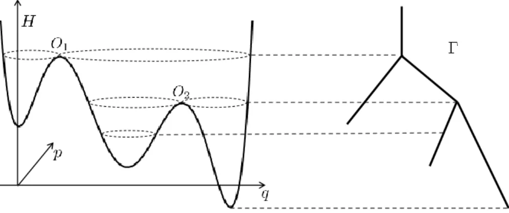
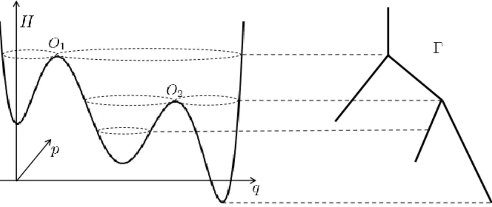
Figure 1: Simulation of (15) for varying ε. Shown are the level curves of the Hamiltonian H and for each case a single trajectory.

where W

t

is a 1-dimensional Wiener process. This system is a prototype for a large class of Hamiltonian systems perturbed by random noise. When the amplitude ε of the noise is small, the dynamics (14) splits into fast and slow components. The fast component approximately follows an unperturbed trajectory of the Hamiltonian system, which is a level set of H . The slow component is visible as a slow modification of the value of H, corresponding to a motion transversal to the level sets of H . Figure 1 illustrates this.

Following [FW94] and others, in order to focus on the slow, Hamiltonian-changing motion, we rescale time such that the Hamiltonian, level-set-following motion is fast, of rate O(1/ε), and the level-set-changing motion is of rate O(1). In other words, the process (15) ‘whizzes round’ level sets of H , while shifting from one level set to another at rate O(1).

This behaviour suggests choosing a coarse-graining map ξ : R

²

→ Γ, which maps a whole level set to a single point in a new space Γ; because of the structure of level sets of H , the set Γ has a structure that is called a graph, a union of one-dimensional intervals locally parametrized by the value of the Hamiltonian.

Figure 2 illustrates this, and in Section 3 we discuss it in full detail.

After projecting onto the graph Γ, the process turns out to behave like a diffusion process on Γ. This property was first made rigorous in [FW94] for a system with one degree of freedom, as here, and non- degenerate noise, using probabilistic techniques. In [FW98] the authors consider the case of degenerate noise by using probabilistic and analytic techniques based on hypoelliptic operators. More recently this problem has been handled using PDE techniques [IS12] (the elliptic case) and Dirichlet forms [BvR14]. In Section 3 we give a new proof, using the structure outlined in Section 1.1.

Figure 2: Left: Hamiltonian R

²

3 (q, p) 7→ H(q, p), Right: Graph Γ

1.3.3 Small-noise limit of a randomly perturbed Hamiltonian system with d degrees of free- dom

The convergence of solutions of (14) as ε → 0 to a diffusion process on a graph requires that the non-perturbed system has a unique invariant measure on each connected component of a level set. While this is true for a Hamiltonian system with one degree of freedom, in the higher-dimensional case one might have additional first integrals of motion. In such a system the slow component will not be a one-dimensional process but a more complicated object—see [FW04]. However, by introducing an additional stochastic perturbation that destroys all first integrals except the Hamiltonian, one can regain the necessary ergodicity, such that the slow dynamics again lives on a graph.

In Section 4 we discuss this case. Equation (14) gains an additional noise term, and reads

∂

_t

ρ = − div(ρJ∇H) + κ div(a∇ρ) + ε∆

_p

ρ, (16)

where a : R

^2d

→ R

^2d×2d

with a∇H = 0, dim(Kernel(a)) = 1 and κ, ε > 0 with κ ε. The spatial domain is R

^2d

, d > 1 with coordinates (q, p) ∈ R

^d

× R

^d

and the unknown is a trajectory in the space of probability measures ρ : [0, T ] → P( R

^2d

). As before the aim is to derive the dynamics as ε → 0. This problem was studied in [FW01] and the results closely mirror the previous case. The main difference lies in the proof of the local equilibrium statement, which we discuss in Section 4.

1.4 Comparison with other work

The novelty of the present paper lies in the following.

1. In comparison with existing literature on the three concrete examples treated in this paper: The results of the three examples are known in the literature (see for instance [Nel67, FW94, FW98, FW01]), but they are proved by different techniques and in a different setting. The variational approach of this paper, which has a clear microscopic interpretation from the large-deviation principle, to these problems is new. We provide alternative proofs, recovering known results, in a unified framework. In addition, we obtain all the results on compactness, local-equilibrium properties and liminf inequalities solely from the variational structures. The approach also is applicable to approximate solutions, which obey the original fine-grained dynamics only to some error. This allows us to work with larger class of measures and to relax many regularity conditions required by the exact solutions. Furthermore, our abstract setting has potential applications to many other systems.

2. In comparison with recently developed variational-evolutionary methods: Many recently developed vari- ational techniques for ‘passing to a limit’ such as the Sandier-Saferty method based on the Ψ-Ψ

^∗

struc- ture [SS04, AMP

⁺

12, Mie14] only apply to gradient flows, i.e. dissipative systems. The approach of this paper also applies to certain variational-evolutionary systems that include non-dissipative effects, such as GENERIC systems [ ¨ Ott05, DPZ13], as in the examples. Since our approach only uses the duality structure of the rate functionals, which holds true for more general systems, we expect that our method works for other limits in non-gradient-flow systems such as the Langevin limit of the Nos´ e-Hoover-Langevin thermostat [FG11, OP11].

3. Quantification of the coarse-graining error. The use of the rate functional as a central ingredient in

‘passing to a limit’ and coarse-graining also allows us to obtain quantitative estimates of the coarse- graining error. One intermediate result of our analysis is a functional inequality similar to the energy- dissipation inequality in the gradient-flow setting (see (4)). This inequality provides an upper bound on the free energy and the integral of the Fisher information by the rate functional and initial free energy.

This offers an alternative to the Talagrand and log-Sobolev inequalities used in the literature [LL10, GOVW09] to obtain quantification of the coarse-graining error. To keep the paper to a reasonable length, we address this issue in details separately in a companion article [DLP

⁺

15].

We provide further comments in Section 5.

1.5 Outline of the article

The rest of the paper is devoted to the study of three concrete problems: the overdamped limit of the VFP equation in Section 2, diffusion on a graph with one degree of freedom in Section 3 and diffusion on a graph with many degrees of freedom in Section 4. In each Section, the main steps in the abstract framework are performed in detail. Section 5 provides further discussion. Finally, detailed proofs of some theorems are given in Appendices A and B.

1.6 Summary of notation

±

_kj

±1, depending on which end vertex O

j

lies of edge I

k

Sec. 3.1

F Free energy (22), (45)

Γ, γ The graph Γ and its elements γ Sec. 3.1

H(·|·) relative entropy (21)

H (q, p) H(q, p) = p

²

/2m + V (q), the Hamiltonian H

ⁿ

n-dimensional Haursdoff measure

I(·|·) relative Fisher Information (24) Int The interior of a set

I

^ε

Large-deviation rate functional for the diffusion-on-graph problem (46) I

^γ

Large-deviation rate functional for the VFP equation (19)

J J =

_−I^{0 I}₀

, the canonical symplectic matrix L Lebesgue measure

M(X ) space of finite, non-negative Borel measures on X P (X ) space of probability measures on X

ˆ

ρ push-forward under ξ of ρ (44)

T (γ) period of the periodic orbit at γ ∈ Γ (48)

V (q) potential on position x x = (q, p) joint variable

ξ

^γ

, ξ coarse-graining maps (30), (43)

Throughout we use measure notation and terminology. For a given topological space X , the space M(X ) is the space of non-negative, finite Borel measures on X; P (X ) is the space of probability measures on X . For a measure ρ ∈ M([0, T ] × R

^2d

), for instance, we often write ρ

t

∈ M( R

^2d

) for the time slice at time t; we also often use both the notation ρ(x)dx and ρ(dx) when ρ is Lebesgue-absolutely-continuous. We equip M(X ) and P (X ) with the narrow topology, in which convergence is characterized by duality with continuous and bounded functions on X .

2 Overdamped Limit of the VFP equation

2.1 Setup of the system

In this section we prove the large-friction limit γ → ∞ of the VFP equation (8). Setting θ = 1 for convenience, and speeding time up by a factor γ, the VFP equation reads

∂

t

ρ = L

ρ^∗

ρ, L

ν^∗

ρ := −γ div ρJ ∇(H + ψ ∗ ν ) + γ

²

div

p

ρ p

m

+ ∆

p

ρ

, (17)

where, as before, J =

_−I^{0 I}₀

and H (q, p) = p

²

/2m + V (q). The spatial domain is R

^2d

with coordinates (q, p) ∈ R

^d

× R

^d

with d ≥ 1, and ρ ∈ C([0, T ]; P( R

^2d

)). For later reference we also mention the primal form of the operator L

ν^∗

:

L

ν

f = γJ∇(H + ψ ∗ ν) · ∇f − γ

²

p

m · ∇

p

f + γ

²

∆

p

f. (18)

We assume

(V1) The potential V ∈ C

²

( R

^d

) has globally bounded second derivative. Furthermore V ≥ 0, |∇V |

²

≤ C(1 + V ) for some C > 0, and e

^−V

∈ L

¹

( R

^d

).

(V2) The interaction potential ψ ∈ C

²

( R

^d

) ∩ L

¹

( R

^d

) is symmetric, has globally bounded first and second derivatives, and the mapping ν 7→ R

ν ∗ ψ dν is convex (and therefore non-negative).

As we described in Section 1.1, the study of the limit γ → ∞ contains the following steps:

1. Prove compactness;

2. Prove a local-equilibrium property;

3. Prove a liminf inequality.

Each of these results is based on the large-deviation structure, which for Equation (17) is

I

^γ

(ρ) = sup

f∈C_b^1,2(R×R^2d)

Z

R^2d

f

_T

dρ

_T

− Z

R^2d

f

₀

dρ

₀

−

T

Z

0

Z

R^2d

∂

_t

f

_t

+ L

ρt

f

_t

dρ

_t

dt − γ

²

2

T

Z

0

Z

R^2d

|∇

p

f

_t

|

²

dρ

_t

dt

. (19)

Alternatively the rate functional can be written as [DPZ13, Theorem 2.5]

I

^γ

(ρ) =



 



 

 1 2

T

Z

0

Z

R^2d

|h

_t

|

²

dρ

_t

dt if ∂

_t

ρ

_t

= L

ρ^∗_t

ρ

_t

− γ div

_p

(ρ

_t

h

_t

), for h ∈ L

²

(0, T ; L

²_∇

(ρ

_t

)),

+∞ otherwise,

(20)

where L

ν

is given in (18), and L

²_∇

(ρ

t

) is the completion of {∇

p

ϕ : ϕ ∈ C

_c^∞

( R

^2d

)} in the ρ

t

-weighted L

²

norm. This second form shows clearly how I

^γ

(ρ) = 0 is equivalent to the property that ρ solves the VFP equation (17). It also shows that if I

^γ

(ρ) > 0 then ρ is an approximative solution in the sense that it satisfies the VFP equation up to some error −γ div

p

(ρ

t

h

t

) whose norm is controlled by the rate functional.

2.2 A priori bounds

We give ourselves a sequence, indexed by γ, of solutions ρ

^γ

to the VFP equation (17) with initial datum ρ

^γ_t

|

t=0

= ρ

0

. We will deduce the compactness of the sequence ρ

^γ

from a priori estimates, that are themselves derived from the rate function I

^γ

.

For nonnegative measures ν, ζ on R

^2d

we first introduce:

• Relative entropy:

H(νkζ) =





 Z

R^2d

[f log f ] dζ if ν = f ζ,

∞ otherwise.

(21)

• The free energy for this system:

F(ν ) := H(ν|Z

_H⁻¹

e

^−H

dx) + 1 2 Z

R^2d

ψ ∗ ν dν = Z

R^2d

h

log g + H + 1 2 ψ ∗ g i

gdx + log Z

H

, (22) where Z

H

= R

e

^−H

and the second expression makes sense whenever ν = gdx.

The convexity of the term involving ψ (condition (V2)) implies that the free energy F is strictly convex and has a unique minimizer µ ∈ P( R

^2d

). This minimizer is a stationary point of the evolution (17), and has the implicit characterization

µ ∈ P( R

^2d

) : µ(dqdp) = Z

⁻¹

exp

−

H(q, p) + (ψ ∗ µ)(q)

dqdp, (23)

where Z is the normalization constant for µ. Note that ∇

p

µ = −µ∇

p

H = −pµ/m.

We also define the relative Fisher Information with respect to µ (in the p-variable only):

I(ν|µ) = sup

ϕ∈C_c^∞(R^2d)

2 Z

R^2d

h

∆

p

ϕ − p

m ∇

p

ϕ − 1

2 |∇

p

ϕ|

²

i

dν. (24)

In the more common case in which the derivatives ∆

p

and ∇

p

are replaced by the full derivatives ∆ and

∇, the relative Fisher Information has an equivalent formulation in terms of the Lebesgue density of ν. In our case such equivalence only holds when ν is absolutely-continuous with respect to the Lebesgue measure in both q and p:

Lemma 2.1 (Equivalence of relative-Fisher-Information expressions for a.c. measures). If ν ∈ P( R

^2d

), ν(dx) = f (x)dx with f ∈ L

¹

( R

^2d

), then

I(ν|µ) =





 Z

R^2d

∇

p

f

f 1

{f >0}

+ p m

2

f dqdp, if ∇

p

f ∈ L

¹_loc

(dqdp),

∞ otherwise,

(25)

where 1

{f >0}

denotes the indicator function of the set {x ∈ R

^2d

| f (x) > 0}.

For a measure of the form ζ(dq)f (p)dp, with ζ 6 dq, I in (24) may be finite while the integral in (25) is not defined. Because of the central role of duality in this paper, definition (24) is a natural one, as we shall see below. The proof of Lemma 2.1 is given in Appendix A.

In the introduction we mentioned that we expect ρ

^γ

to become Maxwellian in the limit γ → ∞. This will be driven by a vanishing relative Fisher Information, as we shall see below. For a.c. measures, the characterization (25) already provides the property

I(f dx|µ) = 0 = ⇒ f (q, p) = ˜ f (q) exp

− p

²

2m

.

This property holds more generally:

Lemma 2.2 (Zero relative Fisher Information implies Maxwellian). If ν ∈ P( R

^2d

) with I(ν|µ) = 0, then there exists σ ∈ P( R

^d

) such that

ν(dqdp) = Z

⁻¹

exp

− p

²

2m

σ(dq)dp,

where Z = R

R^d

e

^−p2/2m

dp is the normalization constant for the Maxwellian distribution.

Proof. From

I(ν |µ) = sup

ϕ∈C_c^∞(R^2d)

2 Z

R^2d

∆

p

ϕ − p

m · ∇

p

ϕ − 1 2 |∇

p

ϕ|

²

dν = 0 (26)

we conclude upon disintegrating ν as ν (dqdp) = σ(dq)ν

q

(dp), for σ-a.e. q: sup

φ∈C_c^∞(R^d)

Z

R^d

∆

_p

φ − p

m · ∇

_p

φ − 1 2 |∇

_p

φ|

²

ν

_q

(dp) = 0.

By replacing φ by λφ, λ > 0, and taking λ → 0 we find

∀φ ∈ C

_c^∞

( R

^d

) : Z

R^d

∆

_p

φ − p m · ∇

p

φ

ν

_q

(dp) = 0, which is the weak form of an elliptic equation on R

^d

with unique solution

ν

q

(dp) = 1 Z exp

− p

²

2m

dp.

This proves the lemma.

In the following theorem we give the central a priori estimate, in which free energy and relative Fisher Information are bounded from above by the rate functional and the relative entropy at initial time.

Theorem 2.3 (A priori bounds). Fix γ > 0 and let ρ ∈ C([0, T ]; P( R

^2d

)) with ρ

_t

|

_t=0

=: ρ

₀

satisfy

I

^γ

(ρ) < ∞, F(ρ

0

) < ∞. (27)

Then for any t ∈ [0, T ] we have

F(ρ

t

) + γ

²

2

Z

t 0

I(ρ

s

|µ) ds ≤ I

^γ

(ρ) + F(ρ

0

). (28)

From (28) we obtain the separate inequality Z

R^2d

H dρ

t

≤ F(ρ

0

) + I

^γ

(ρ) − log Z

R^2d

e

^−H

. (29)

This estimate will lead to a priori bounds in two ways. First, the bound on the free energy gives tightness estimates, and therefore compactness in space (Theorem 2.4); secondly, the relative Fisher Information is bounded by C/γ

²

and therefore vanishes in the limit γ → ∞. This fact is used to prove that the limiting measure is Maxwellian (Lemma 2.5).

Proof. We give a heuristic motivation here; Appendix B contains a full proof. Given a trajectory ρ as in the theorem, note that by (20) ρ satisfies

∂

t

ρ

t

= −γ div ρ

t

J ∇(H + ψ ∗ ρ

t

) + γ

²

div

p

ρ

t

p

m + ∆

p

ρ

t

− γ div

p

ρ

t

h

t

. We then formally calculate

d

dt F(ρ

t

) = Z

R^2d

log ρ

t

+ 1 + H + ψ ∗ ρ

t

−γ div ρ

t

J∇(H + ψ ∗ ρ

t

) + γ

²

div

p

ρ

t

p

m + ∆

p

ρ

t

− γ div

_p

ρ

_t

h

_t

= −γ

²

Z

R^2d

1 ρ

t

∇

p

ρ

_t

+ ρ

_t

p m

2

+ γ Z

R^2d

h

_t

∇

p

ρ

_t

+ ρ

_t

p m

≤ − γ

²

2

Z

R^2d

1 ρ

t

∇

_p

ρ

_t

+ ρ

_t

p m

2

+ 1 2

Z

R^2d

ρ

_t

h

²_t

,

where the first O(γ) term cancels because of the antisymmetry of J . After integration in time this latter expression yields (28).

For exact solutions of the VFP equation, i.e. when I

^γ

(ρ) = 0, this argument can be made rigorous following e.g. [BCS97]. However, the fairly low regularity of the right-hand side in (20) prevents these techniques from working. ‘Mild’ solutions, defined using the variation-of-constants formula and the Green function for the hypoelliptic operator, are not well-defined either, for the same reason: the term RR

∇

p

G·h dρ

that appears in such an expression is generally not integrable. In the appendix we give a different proof,

using the method of dual equations.

2.3 Coarse-graining and compactness

As we described in the introduction, in the overdamped limit γ → ∞ we expect that ρ will resemble a Maxwellian distribution Z

⁻¹

exp −p

²

/2m

σ

t

(dq), and that the q-dependent part σ will solve the Vlasov- Fokker-Planck equation (12). We will prove this statement using the method described in Section 1.1.

It would be natural to define ‘coarse-graining’ in this context as the projection ξ(q, p) := q, since that should eliminate the fast dynamics of p and focus on the slower dynamics of q. However, this choice fails: it completely decouples the dynamics of q from that of p, thereby preventing the noise in p from transferring to q. Following the lead of Kramers [Kra40], therefore, we define a slightly different coarse-graining map

ξ

^γ

: R

^2d

→ R

^d

, ξ

^γ

(q, p) := q + p

γ . (30)

In the limit γ → ∞, ξ

^γ

→ ξ locally uniformly, recovering the projection onto the q-coordinate.

The theorem below gives the compactness properties of the solutions ρ

^γ

of the rescaled VFP equation that allow us to pass to the limit. There are two levels of compactness, a weaker one in the original space R

^2d

, and a stronger one in the coarse-grained space R

^d

= ξ

^γ

( R

^2d

). This is similar to other multilevel compactness results as in e.g. [GOVW09].

Theorem 2.4 (Compactness). Let a sequence ρ

^γ

∈ C([0, T ]; P ( R

^2d

)) satisfy for a suitable constant C > 0 and every γ the estimate

I

^γ

(ρ

^γ

) + F(ρ

^γ_t

|

t=0

) ≤ C. (31) Then there exist a subsequence (not relabelled) such that

1. ρ

^γ

→ ρ in M([0, T ] × R

^2d

) with respect to the narrow topology.

2. ξ

_#^γ

ρ

^γ

→ ξ

_#

ρ in C([0, T ]; P ( R

^d

)) with respect to the uniform topology in time and narrow topology on P ( R

^d

).

For a.e. t ∈ [0, T ] the limit ρ

_t

satisfies

I(ρ

t

|µ) = 0 (32)

Proof. To prove part 1, note that the positivity of the convolution integral involving ψ and the free-energy- dissipation inequality (28) imply that H(ρ

^γ_t

|Z

_H⁻¹

e

^−H

dx) is bounded uniformly in t and γ. By an argument as in [ASZ09, Prop. 4.2] this implies that {ρ

^γ_t

: t ∈ [0, T ], γ > 1} is tight, upon which compactness in M([0, T ] × R

^2d

) follows.

To prove (32) we remark that

0 ≤ sup

ϕ∈C_c^∞(R×R^2d)

2 Z

T

0

Z

R^2d

h

∆

_p

ϕ − p

m ∇

_p

ϕ − 1

2 |∇

_p

ϕ|

²

i

dρ

^γ_t

dt ≤ Z

T

0

I (ρ

^γ_t

|µ) dt ≤ C γ

²

γ→∞

−→ 0,

and by passing to the limit on the left-hand side we find sup

ϕ∈C_c^∞(R×R^2d)

2 Z

T

0

Z

R^2d

h

∆

p

ϕ − p

m ∇

p

ϕ − 1

2 |∇

p

ϕ|

²

i

dρ

t

dt = 0.

By disintegrating ρ in time as ρ(dtdqdp) = ρ

_t

(dqdp)dt, we find that I(ρ

_t

|µ) = 0 for (Lebesgue-) almost all t.

We prove part 2 with the Arzel` a-Ascoli theorem. For any t ∈ [0, T ] the sequence ξ

_#^γ

ρ

^γ_t

is tight, which follows from the tightness of ρ

^γ_t

proved above and the local uniform convergence ξ

^γ

→ ξ (see e.g. [AGS08, Lemma 5.2.1]).

To prove equicontinuity we will show sup

γ>1

sup

t∈[0,T−h]

sup

ϕ∈C_c²(R^d) kϕk_{C2 (R}d)≤1

Z

R^d

ϕ(ξ

_#^γ

ρ

^γ_t+h

− ξ

^γ_#

ρ

^γ_t

) −−−→

^h→0

0. (33)

Note that the boundedness of the rate functional, definition (20), and tightness of ρ

^γ

imply that there esxists some h

^γ

∈ L

²

(0, T ; L

²_∇

(ρ

^γ_t

)) with

∂

t

ρ

^γ_t

= (L

_ρ^γ

t

)

^∗

ρ

^γ_t

− γ div

p

(ρ

^γ_t

h

^γ_t

). (34)

in duality with C

_b²

( R

^2d

). Therefore for any f ∈ C

_b²

( R

^2d

) we have in the sense of distributions on [0, T ], d

dt Z

R^2d

f ρ

^γ_t

= Z

R^2d

γ p

m · ∇

q

f − γ∇

q

V · ∇

p

f − γ∇

p

f · (∇

q

ψ ∗ ρ

^γ

) − γ

²

p

m · ∇

p

f + γ

²

∆

p

f + γ∇

p

f · h

^γ_t

)

dρ

^γ_t

.

To prove (33), make the choice f = ϕ ◦ ξ

^γ

for ϕ ∈ C

_c²

( R

^d

) and integrate over [t, t + h] to arrive at Z

R^d

ϕ(ξ

^γ_#

ρ

^γ_t+h

− ξ

_#^γ

ρ

^γ_t

) = Z

t+h

t

Z

R^2d

− ∇V (q) · ∇ϕ

q + p γ

− (∇

q

ψ ∗ ρ

^γ_s

)(q) · ∇ϕ

q + p γ

+ ∆ϕ

q + p γ

+ ∇ϕ

q + p

γ

· h

^γ_s

(q, p)

dρ

^γ_s

ds.

We estimate the first term on the right hand side by using H¨ older’s inequality and growth condition (V1),

Z

t+h t

Z

R^2d

∇V (q) · ∇ϕ

q + p γ

dρ

^γ_s

ds

≤ k∇ϕk

_∞

√ h

Z

t+h t

Z

R^2d

|∇V (q)|

²

dρ

^γ_s

ds

!

1/2

≤k∇ϕk

_∞

√ h

Z

t+h t

Z

R^2d

C(1 + V (q))ρ

^γ_s

ds

!

1/2

≤ Ck∇ϕk ˜

_∞

h

where the last inequality follows from the free-energy-dissipation inequality (28). For the second term we use |∇

q

ψ ∗ ρ

^γ_s

| ≤ k∇

q

ψk

_∞

and the last term is estimated by H¨ older’s inequality,

Z

t+h t

Z

R^2d

∇ϕ

q + p γ

h

^γ_s

(q, p)dρ

^γ_s

ds

≤ k∇ϕk

_∞

√ h

Z

t+h t

Z

R^2d

|h

^γ_s

|

²

dρ

^γ_s

ds

¹₂

≤k∇ϕk

_∞

√

h (2I

^γ

(ρ

^γ

))

¹²

≤ Ck∇ϕk

_∞

√ h.

To sum up we have

Z

R^d

ϕ(ξ

_#^γ

ρ

^γ_t+h

− ξ

_#^γ

ρ

^γ_t

)

≤ C √

h −−−→

^h→0

0, where C is independent of t and γ.

Thus by the Arzel` a-Ascoli theorem there exists a ν ∈ C([0, T ]; P( R

^d

)) such that ξ

^γ_#

ρ

^γ

→ ν with respect to uniform topology in time and narrow topology on P ( R

^d

). Since ρ

^γ

→ ρ in M([0, T ] × R

^2d

) and ξ

^γ

→ ξ locally uniformly, we have ξ

_#^γ

ρ

^γ

→ ξ

#

ρ in M([0, T ] × R

^d

) (again using [AGS08, Lemma 5.2.1]), implying that ν = ξ

#

ρ. This concludes the proof of Theorem 2.4.

2.4 Local equilibrium

A central step in any coarse-graining method is the treatment of the information that is ‘lost’ upon coarse- graining. The lemma below uses the a priori estimate (28) to reconstruct this information, which for this system means showing that ρ

^γ

becomes Maxwellian in p as γ → ∞.

Lemma 2.5 (Local equilibrium). Under the same conditions as in Theorem 2.4 let us assume that ρ

^γ

→ ρ in M([0, T ]× R

^2d

) with respect to the narrow topology. Then there exists σ ∈ M([0, T ]× R

^d

), σ(dtdq) = σ

t

(dq)dt, such that for allmost all t ∈ [0, T ],

ρ

t

(dqdp) = Z

⁻¹

exp

− p

²

2m

σ

t

(dq)dp, (35)

where Z = R

R^d

e

^−p2/2m

dp is the normalization constant for the Maxwellian distribution. Furthermore ξ

_#^γ

ρ

^γ_t

→ σ

t

narrowly for every t ∈ [0, T ].

Proof. Since ρ

^γ

→ ρ narrowly in M([0, T ]× R

^2d

), the limit ρ also has the disintegration structure ρ(dtdpdq) = ρ

t

(dpdq)dt, with ρ

t

∈ P( R

^2d

). From the a priori estimate (28) and the duality definition of I we have I(ρ

t

|µ) = 0 for almost all t, and the characterization (35) then follows from Lemma 2.2. The compactness results in Theorem 2.4 imply that ξ

_#^γ

ρ

^γ_t

→ ξ

#

ρ

t

= σ

t

for all t ∈ [0, T ].

2.5 Liminf inequality

The final step in the variational technique is proving an appropriate liminf inequality which also provides the structure of the limiting coarse-grained evolution. The following theorem makes this step rigorous.

Define the (limiting) functional I : C([0, T ]; P ( R

^d

)) → R by I(σ) := sup

g∈C_b^1,2(R×R^d)

Z

R^d

g

_T

dσ

_T

− Z

R^d

g

₀

dσ

₀

− Z

T

0

Z

R^d

∂

_t

g − ∇V · ∇g − (∇ψ ∗ σ) · ∇g + ∆g dσ

_t

dt

− 1 2

Z

T 0

Z

R^d

|∇g|

²

dσ

_t

dt. (36) Note that I ≥ 0 (since g = 0 is admissible); we have the equivalence

I(σ) = 0 ⇐⇒ ∂

t

σ = div σ∇V (q) + div σ(∇ψ ∗ σ) + ∆σ in [0, T ] × R

^d

.

Theorem 2.6 (Liminf inequality). Under the same conditions as in Theorem 2.4 we assume that ρ

^γ

→ ρ narrowly in M([0, T ] × R

^2d

) and ξ

^γ_#

ρ

^γ

→ ξ

#

ρ ≡ σ in C([0, T ]; P( R

^d

)). Then

lim inf

γ→∞

I

^γ

(ρ

^γ

) ≥ I(σ).

Proof. Write the large deviation rate functional I

^γ

: C([0, T ]; P ( R

^2d

)) → R in (19) as I

^γ

(ρ) = sup

f∈C_b^1,2(R×R^2d)

J

^γ

(ρ, f), (37)

where J

^γ

(ρ, f ) =

Z

R^2d

f

T

dρ

T

− Z

R^2d

f

0

dρ

0

− Z

T

0

Z

R^2d

∂

t

f + γ p

m · ∇

q

f − γ∇

q

V · ∇

p

f − γ∇

p

f · (∇

q

ψ ∗ ρ

t

)

− γ

²

p

m · ∇

p

f + γ

²

∆

p

f

dρ

t

dt − γ

²

2

Z

T 0

Z

R^2d

|∇

p

f |

²

dρ

t

dt.

Define A := {f = g ◦ ξ

^γ

with g ∈ C

_b^1,2

( R × R

^d

)}. Then we have

I

^γ

(ρ

^γ

) ≥ sup

f∈A

J

^γ

(ρ

^γ

, f), and

J

^γ

(ρ

^γ

, g ◦ ξ

^γ

) = Z

R^2d

g

T

◦ ξ

^γ

dρ

^γ_T

− Z

R^2d

g

0

◦ ξ

^γ

dρ

^γ₀

− Z

T

0

Z

R^2d

∂

t

(g ◦ ξ

^γ

) − ∇

q

V (q) · ∇g

q + p γ

+ ∆g

q + p γ

− ∇g

q + p γ

· (∇

q

ψ ∗ ρ

^γ_t

)(q)

dρ

^γ_t

dt − 1 2

Z

T 0

Z

R^2d

|∇(g ◦ ξ

^γ

)|

²

dρ

^γ_t

dt. (38)

Note how the specific dependence of ξ

^γ

(q, p) = q + p/γ on γ has caused the coefficients γ and γ

²

in the expression above to vanish. Adding and subtracting ∇V (q+p/γ)·∇g(q+p/γ) in (38) and defining ˆ ρ

^γ

:= ξ

_#^γ

ρ

^γ

, J

^γ

can be rewritten as

J

^γ

(ρ, g ◦ ξ

^γ

) = Z

R^d

g

T

dˆ ρ

^γ_T

− Z

R^d

g

0

dˆ ρ

^γ₀

− Z

T

0

Z

R^d

(∂

t

g − ∇V · ∇g + ∆g) (ζ) ˆ ρ

^γ_t

(dζ)dt − 1 2

Z

T 0

Z

R^d

|∇g|

²

dˆ ρ

^γ_t

dt

− Z

T

0

Z

R^2d

∇V

q + p γ

− ∇V (q)

· ∇g

q + p γ

dρ

^γ_t

dt + Z

T

0

Z

R^2d

∇g

q + p γ

· (∇

q

ψ ∗ ρ

^γ_t

)(q)dρ

^γ_t

dt.

(39) We now show that (39) converges to the right-hand side of (36), term by term. Since ξ

_#^γ

ρ

^γ

→ ξ

_#

ρ = σ narrowly in M([0, T ] × R

^2d

) and g ∈ C

_b²

( R × R

^d

) we have

Z

T 0

Z

R^d

∂

t

g − ∇V · ∇g + ∆g + 1 2 |∇g|

²

dˆ ρ

^γ_t

dt −

^γ→∞

−−− → Z

T

0

Z

R^d

∂

t

g − ∇V · ∇g + ∆g + 1 2 |∇g|

²

dσ

t

dt.

Taylor expansion of ∇V around q and estimate (29) give

Z

T 0

Z

R^2d

∇V

q + p γ

− ∇V (q)

· ∇g

q + p γ

dρ

^γ_t

dt

≤

≤ kD

²

V k

∞

k∇gk

∞

√ T

Z

T 0

Z

R^2d

p

²

γ

²

dρ

^γ_t

dt

!

^1/2

≤ C γ

−

γ→∞

−−− → 0.

Adding and subtracting ∇g(q) · (∇

q

ψ ∗ ρ

^γ_t

)(q) in (39) we find Z

T

0

Z

R^2d

∇g

q + p γ

· (∇

q

ψ ∗ ρ

^γ_t

)(q)dρ

^γ_t

dt = Z

T

0

Z

R^2d

∇g(q) · (∇

q

ψ ∗ ρ

^γ_t

)(q)dρ

^γ_t

dt +

Z

T 0

Z

R^2d

∇g

q + p γ

− ∇g(q)

· (∇

_q

ψ ∗ ρ

^γ_t

)(q)dρ

^γ_t

dt.

Since ρ

^γ

→ ρ we have ρ

^γ

⊗ ρ

^γ

→ ρ ⊗ ρ and therefore passing to the limit in the first term and using the local-equilibrium characterization of Lemma 2.5, we obtain

Z

T 0

Z

R^2d

∇g(q) · (∇

q

ψ ∗ ρ

^γ

)(q) dρ

^γ_t

dt −−−→

^γ→0

Z

T

0

Z

R^d

∇g · (∇ψ ∗ σ) dσ

_t

dt.

For the second term we calculate

Z

T 0

Z

R^2d

∇g

q + p γ

− ∇g(q)

· (∇

q

ψ ∗ ρ

^γ

)(q)dρ

^γ_t

dt

≤kD

²

gk

∞

k∇

q

ψk

∞

√ T

Z

T 0

Z

R^2d

p

²

γ

²

dρ

^γ_t

dt

!

^1/2

≤ C γ

−

γ→∞

−−− → 0.

Therefore Z

T

0

Z

R^2d

∇g

q + p γ

· (∇

q

ψ∗ρ

^γ

)(q)dρ

^γ_t

dt −

^γ→∞

−−− → Z

T

0

Z

R^d

∇g · (∇ψ ∗ σ) dσ

t

dt.

2.6 Discussion

The ingredients of the convergence proof above are, as mentioned before, (a) a compactness result, (b) a local-equilibrium result, and (c) a liminf inequality. All three follow from the large-deviation structure, through the rate functional I

^γ

. We now comment on these.

Compactness. Compactness in the sense of measures is, both for ρ

^γ

and for ξ

_#^γ

ρ

^γ

, a simple consequence of the confinement provided by the growth of H . In Theorem 2.4 we provide a stronger statement for ξ

_#^γ

ρ

^γ

, by showing continuity in time, in order for the limiting functional I(σ) in (36) to be well defined. This continuity depends on the boundedness of I

^γ

.

Local equilibrium. The local-equilibrium statement depends crucially on the structure of I

^γ

, and more specifically on the large coefficient γ

²

multiplying the derivatives in p. This coefficient also ends up as a prefactor of the relative Fisher Information in the a priori estimate (28), and through this estimate it drives the local-equilibrium result.

Liminf inequality. As remarked in the introduction, the duality structure of I

^γ

is the key to the liminf inequality, as it allows for relatively weak convergence of ρ

^γ

and ξ

_#^γ

ρ

^γ

. The role of the local equilibrium is to allow us to replace the p-dependence in some of the integrals by the Maxwellian dependence, and therefore to reduce all terms to dependence on the macroscopic information ξ

_#^γ

ρ

^γ

only.

As we have shown, the choice of the coarse-graining map has the advantage that it has caused the (large) coefficients γ and γ

²

in the expression of the rate functionals to vanish. In other words, it cancels out the inertial effects and transforms a Laplacian in p variable to a Laplacian in the coarse-grained variable while rescaling it to be of order 1. The choice ξ(q, p) = q, on the other hand, would lose too much information by completely discarding the diffusion.

3 Diffusion on a Graph, d = 1

In this section we derive the small-noise limit of a randomly perturbed Hamiltonian system, which corre- sponds to passing to the limit ε → 0 in (14). In terms of a rescaled time, in order to focus on the time scale of the noise, equation (14) becomes

∂

t

ρ

^ε

= − 1

ε div(ρ

^ε

J∇H) + ∆

p

ρ

^ε

. (40)

Here ρ

^ε

∈ C([0, T ], P ( R

²

)), J =

_{−1 0}^{0 1}

is again the canonical symplectic matrix, ∆

p

is the Laplacian in the p-direction, and the equation holds in the sense of distributions. The Hamiltonian H ∈ C

²

( R

^2d

; R ) is again defined by H (q, p) = p

²

/2m + V (q) for some potential V : R

^d

→ R . We make the following assumptions (that we formulate on H for convenience):

(A1) H ≥ 0, and H is coercive, i.e. H (x) −−−−→ ∞;

^|x|→∞

(A2) |∇H |, |∆H |, |∇

p

H |

²

≤ C(1 + H);

(A3) H has a finite number of non-degenerate (i.e. non-singular Hessian) saddle points O

₁

, . . . , O

_n

with H (O

i

) 6= H (O

j

) for every i, j ∈ {1, . . . , n}, i 6= j.

As explained in the introduction, and in contrast to the VFP equation of the previous section, equa- tion (40) has two equally valid interpretations: as a PDE in its own right, or as the Fokker-Planck (forward Kolmogorov) equation of the stochastic process

X

^ε

= Q

^ε

P

^ε

, dX

_t^ε

= 1

ε J ∇H(X

_t^ε

)dt + √ 2

0 1

dW

t

. (41)

For the sequel we will think of ρ

^ε

as the law of the process X

_t^ε

; although this is not strictly necessary, it

helps in illustrating the ideas.