WCET analysis and optimization for multi-core real-time systems

WCET Analysis and Optimization for Multi-Core Real-Time Systems

Dissertation

zur Erlangung des Grades eines

Doktors der Ingenieurwissenschaften

der Technischen Universität Dortmund an der Fakultät für Informatik

von Timon Kelter

Dortmund

2015

Tag der mündlichen Prüfung: 12. März 2015

Dekan / Dekanin: Prof. Dr. Gernot Fink Gutachter / Gutachterinnen: Prof. Dr. Peter Marwedel

Prof. Dr. Isabelle Puaut

Acknowledgments

First and foremost I want to thank my advisor Prof. Dr. Peter Marwedel for pointing my research into a rewarding direction from the start on and for providing me with the opportunity to work on this fascinating field of research in an inspiring, international team. Without his continued support this thesis would not exist. I would also like to thank Prof. Dr. Isabelle Puaut for her time and commitment to review this thesis.

The implementation of the WCET analyzer and the WCET optimizations which are presented in this thesis would not have been possible without the previous work of numerous colleagues at our chair over the course of more than one decade. I am especially grateful for the provision of the WCC framework, on which the majority of my practical work was built. In this context, I owe special thanks to Prof. Dr. Heiko Falk for being one of the most thorough reviewers and advisors I have ever met, to Dr. Paul Lokuciejewski for introducing me to this interesting field of research, to Dr.

Sascha Plazar for being a fantastic office neighbor, to Jan Christopher Kleinsorge for our mutual motivation to finish the PhD project and to all of them for the enjoyable time in countless on- and off-topic disucssions.

For proof-reading my drafts and papers, for helpful discussions and for being re- ally good colleagues I would also like to thank Björn Bönninghoff, Olaf Neugebauer, Pascal Libuschewski, Chen-Wei Huang, Dr. Michael Engel, Helena Kotthaus, An- dreas Heinig, Florian Schmoll and Dr. Daniel Cordes. On the implementation side, my work was supported by Jan Körtner, Hendrik Borghorst, Tim Harde, Chris- tian Günter and Henning Garus. Without their help the whole WCET analyzer implementation would be in a different shape now.

Furthermore, I am deeply thankful towards the former WCET analysis team at the National University of Singapore, most of all to Dr. Sudipta Chattopadhyay and Prof. Dr. Abhik Roychoudhury, for giving me the opportunity to work on the Chronos WCET analyzer. Without these first steps I possibly would have not found my way into the topic of WCET analysis.

What has kept me going in the last years was of course not only scientific progress but also the support that I received from friends and family, who kept me grounded when my thoughts were spinning around work issues. Many thanks to all of you – you know who you are. In particular I owe my father a big debt of gratitude for motivating me to pick up computer science as a profession and to finally strive for the PhD.

iii

Abstract

During the design of safety-critical real-time systems, developers must be able to verify that a system shows a timely reaction to external events. To achieve this, the Worst-Case Execution Time (WCET) of each task in such a system must be determined. The WCET is used in the schedulability analysis in order to verify that all tasks will meet their deadlines and to verify the overall timing of the system.

Unfortunately, the execution time of a task depends on the task’s input values, the initial system state, the preemptions due to tasks executing on the same core and on the interference due to tasks executing in parallel on other cores. These dependencies render it close to impossible to cover every feasible timing behavior in measurements. It is preferable to create a static analysis which determines the WCET based on a safe mathematical model.

The static WCET analysis tools which are currently available are restricted to a single task running uninterruptedly on a single-core system. There are also exten- sions of these tools which can capture the effects of multi-tasking, i.e., preemptions by higher-priority tasks, on the WCET for certain well-defined scenarios. These tools are nowadays already used to verify industrial real-time software, e.g., in the automotive and avionics domain. Up to now, there are no mature tools which can handle the case of parallel tasks on a multi-core platform, where the tasks potentially interfere with each other.

This dissertation presents multiple approaches towards a WCET analysis for different types of multi-core systems. They are based upon previous work on the modeling of hardware and program behavior but extend it to the treatment of shared resources like shared caches and shared buses. We present multiple methods of inte- grating shared bus analysis into the classical WCET analysis framework and show that time-triggered bus arbitration policies can be efficiently analyzed with high pre- cision. In order to get precise WCET estimations for the case of shared caches, we present an efficient analysis of interactions in parallel systems which utilizes timing information to cut down the search space. All of the analyses were implemented in a research C compiler. Extensive evaluations on real-time benchmarks show that they are up to 11 . 96 times more precise than previous approaches.

Finally, we present two compiler optimizations which are tailored towards the optimization of the WCET of tasks in multi-core systems, namely an evolutionary optimization of shared resource schedules and an instruction scheduling which uses WCET analysis results to optimally place shared resource requests of individual tasks. Experiments show that the two combined optimizations are able to achieve an average WCET reduction of 33% .

During the course of this thesis, a complete WCET analysis framework was developed which can be used for further work like the integration of multi-task and multi-core-aware techniques into a single analyzer.

v

Publications

Parts of this thesis have been published in journals and the proceedings of the following conferences and workshops (in chronological order):

Timon Kelter, Heiko Falk, Peter Marwedel, Sudipta Chattopadhyay, and Abhik Roychoud- hury. “Bus-Aware Multicore WCET Analysis through TDMA Offset Bounds”. In: Pro- ceedings of the 23rd Euromicro Conference on Real-Time Systems (ECRTS). Porto, Portugal, 07/2011, pp. 3–12.

Sudipta Chattopadhyay, Chong Lee Kee, Abhik Roychoudhury, Timon Kelter, Heiko Falk, and Peter Marwedel. “A Unified WCET Analysis Framework for Multi-Core Platforms”.

In: IEEE Real-Time and Embedded Technology and Applications Symposium (RTAS).

Beijing, China, 04/2012, pp. 99–108.

Timon Kelter, Tim Harde, Peter Marwedel, and Heiko Falk. “Evaluation of Resource Ar- bitration Methods for Multi-Core Real-Time Systems”. In: Proceedings of the 13th In- ternational Workshop on Worst-Case Execution Time Analysis (WCET). Ed. by Claire Maiza. Paris, France, 07/2013.

Timon Kelter, Heiko Falk, Peter Marwedel, Sudipta Chattopadhyay, and Abhik Roychoud- hury. “Static Analysis of Multi-Core TDMA Resource Arbitration Delays”. English.

In: Real-Time Systems 50.2 (03/2014), pp. 185–229. issn: 0922-6443. doi: 10.1007/

s11241-013-9189-x. url: http://dx.doi.org/10.1007/s11241-013-9189-x.

Sudipta Chattopadhyay, Lee Kee Chong, Abhik Roychoudhury, Timon Kelter, Peter Mar- wedel, and Heiko Falk. “A Unified WCET Analysis Framework for Multicore Platforms”.

In: ACM Transactions on Embedded Computing Systems 13.4s (04/2014), 124:1–124:29.

issn : 1539-9087. doi : 10 . 1145 / 2584654. url : http : / / doi . acm . org / 10 . 1145 / 2584654.

Timon Kelter, Peter Marwedel, and Hendrik Borghorst. “WCET-aware Scheduling Opti- mizations for Multi-Core Real-Time Systems”. In: International Conference on Em- bedded Computer Systems: Architectures, Modeling, and Simulation (SAMOS). Samos, Greece, 07/2014.

Chen-Wei Huang, Timon Kelter, Bjoern Boenninghoff, Jan Kleinsorge, Michael Engel, Peter Marwedel, and Shiao-Li Tsao. “Static WCET Analysis of the H.264/AVC Decoder Ex- ploiting Coding Information”. In: International Conference on Embedded and Real-Time Computing Systems and Applications (RTCSA). IEEE. Chongqing, China, 08/2014.

Timon Kelter and Peter Marwedel. “Parallelism Analysis: Precise WCET Values for Com- plex Multi-Core Systems”. In: Third International Workshop on Formal Techniques for Safety-Critical Systems (FTSCS). Ed. by Cyrille Artho and Peter Ölveczky. Luxem- bourg: Springer, 11/2014.

vii

Contents

1 Introduction 1

1.1 Motivation . . . . 3

1.2 Contributions of this Work . . . . 7

1.3 Organization of the Thesis . . . . 8

1.4 Author’s Contribution to this Dissertation . . . . 9

2 Timing Analysis Concepts 11 2.1 Abstract Interpretation . . . . 12

2.2 WCET Analysis for Uninterrupted Single Tasks . . . . 18

2.2.1 Static WCET Analysis . . . . 19

2.2.2 Parametric WCET analysis . . . . 21

2.2.3 Hybrid WCET analysis . . . . 21

2.2.4 Early-Stage WCET analysis . . . . 22

2.2.5 Statistical WCET analysis . . . . 22

2.2.6 WCET-friendly Hardware Design . . . . 23

2.2.7 Experiences with Practical Application of WCET Analysis 23 2.2.8 Timing Anomalies . . . . 24

2.2.9 Compositionality in WCET Analysis . . . . 27

2.3 Timing Analysis of Sequential Multi-Task Systems . . . . 29

2.3.1 Accounting for the Timing Behavior of System Calls . . . 29

2.3.2 Accounting for Task Interaction Impacts on the WCET . 30 2.3.3 Schedulability of Multi-Task Systems with Given WCETs 32 2.4 Timing Analysis of Parallel Multi-Task Systems . . . . 32

2.4.1 Multi-Core Systems . . . . 33

2.4.2 Distributed Systems . . . . 34

3 WCC Framework 37 3.1 Related Work . . . . 38

3.2 Compiler Phases . . . . 39

3.3 Flow Fact Management . . . . 41

3.4 System Model . . . . 43

3.5 Extensions for Binary Input Files . . . . 47

4 Single-Core WCET-Analysis 51 4.1 IPCFG Construction . . . . 52

4.1.1 Analysis Graph . . . . 54

4.1.2 Context Graph . . . . 55

4.2 Value Analysis . . . . 60

4.2.1 Abstract Value Domain . . . . 60

ix

x Contents

4.2.2 Challenges of Predicated Execution . . . . 62

4.3 Microarchitectural Analysis . . . . 63

4.3.1 ARM7TDMI Pipeline Model . . . . 67

4.3.2 Cache Analysis . . . . 70

4.4 Path Analysis . . . . 73

4.5 Evaluation . . . . 76

5 Multi-Core WCET Analysis 81 5.1 Introduction . . . . 82

5.2 Multi-Core Challenges . . . . 82

5.2.1 Shared Caches . . . . 82

5.2.2 Shared Interconnection Structures . . . . 83

5.3 Related Work . . . . 86

5.3.1 WCET Analysis Approaches for Multi-Cores . . . . 86

5.3.2 WCET-friendly Multi-Core Architecture Design . . . . 89

5.4 Partitioned Multi-Core WCET Analysis . . . . 90

5.4.1 Shared Cache Handling . . . . 91

5.4.2 Shared Bus Analysis Preliminaries . . . . 94

5.4.3 Basic Bus Domains . . . . 96

5.4.4 Loop Unrolling . . . . 100

5.4.5 Offset Contexts . . . . 101

5.4.6 Offset Relocation . . . . 104

5.4.7 Timing-Anomaly-Free Analysis . . . . 110

5.4.8 Evaluation . . . . 113

5.5 Unified WCET Analysis for Complex Multi-Cores . . . . 120

5.5.1 Related Work . . . . 120

5.5.2 Task Model . . . . 123

5.5.3 Motivating Example . . . . 123

5.5.4 Prerequisites . . . . 126

5.5.5 Parallel Execution Graph Construction . . . . 127

5.5.6 Parallel System States . . . . 132

5.5.7 Correctness . . . . 135

5.5.8 Extensions . . . . 138

5.5.9 Evaluation . . . . 140

5.6 Summary . . . . 144

6 Multi-Core WCET Optimization 147 6.1 Multi-Objective Evolutionary Schedule Optimization . . . . 147

6.1.1 Related Work . . . . 148

6.1.2 Evolutionary Algorithm . . . . 148

6.1.3 Evaluation . . . . 150

6.2 WCET-driven Multi-Core Instruction Scheduling . . . . 154

6.2.1 Related Work . . . . 155

Contents xi

6.2.2 Scheduling Heuristics . . . . 156 6.2.3 Evaluation . . . . 158 6.3 Summary . . . . 160

7 Conclusion and Future Work 163

7.1 Summary . . . . 163 7.2 Future Work . . . . 165

List of Figures 169

List of Tables 169

List of Algorithms 171

Glossary 173

Bibliography 175

A Employed Benchmarks 209

Chapter 1

Introduction

This dissertation deals with an aspect of computer science that has been a second- class citizen since the emergence of the discipline: With time. Or, to put it more precisely, with safe bounds on the timing behavior of programs running on a com- puter system.

Since the days of mainframes, attempts have been made to increase the pro- ductivity of a programmer by supplying him with ever more powerful program- ming languages and compilers for the latter [Myc07], by teaching useful idioms and patterns [GHJ+95] and by making the single computers faster to allow the soft- ware complexity to increase steadily [Sch97]. The runtime behavior of algorithms has traditionally been classified asymptotically in big O notation which eases or even enables the reasoning about runtime behavior for complex algorithms [Weg03].

For many computer applications the asymptotical classification is sufficient, even though its limitations are already stressed by examples like the Simplex algorithm, which in spite of having exponential asymptotical runtime performs better than its polynomial-time counterparts on most real-world examples [Cor10, Choosing an optimizer for your LP problem].

The major shortcoming of this type of runtime classification is that it is not us- able in the important area of real-time systems, i.e., computer systems in which the executed tasks must always fulfill their work in a bounded time interval or before a given deadline. An asymptotic modeling which ignores constant factors in the run- time formula is not applicable here, since taking twice the allowed time or only once is an important difference, possibly rendering the system dysfunctional in the former case. Most real-time systems are also embedded systems, i.e., “information processing systems embedded into enclosing products” [Mar11], which are integrated into many devices of daily life. Application domains for embedded systems are numerous and cover areas like automotive electronics, avionics, railways, telecommunication, the health sector, security, consumer-electronics, fabrication equipment, smart build- ings, logistics, robotics, military applications, and many more [Mar11].

Real-time systems are generally classified as soft or hard real-time systems, where

“soft” means that deadlines may be violated for a few executions of a task, but not regularly and “hard” means that not a single deadline must be violated. Multimedia applications like audio and video decoders are prime examples for soft real-time sys- tems, whereas industrial Electronic Control Units (ECU) in robotics, power stations, cars and planes are typical hard-real time systems. Modern cars for example have more than 70 ECUs [ES08] for engine control, safety features like anti-lock braking

1

2 Chapter 1. Introduction

Model-driven Design ( ASCET , SCADE , ...)

Coding Conventions (MISRA-C, ...)

Standardization and Re-use (OSEK, AUTOSAR, ...) Real-Time

System Design Formal Verification

( Astrée , Model checking, abstract interpretation, ...)

Testing (Unit tests, In- tegration Tests, Coverage Criteria, ...)

WCET Analysis ( aiT , Static, Dy- namic, Hybrid, ...) Schedulability Analysis

(Real-Time Calculus, Static schedulabil-

ity theorems, ...) Figure 1.1: Real-time system verification tools.

and electronic stability program and multi-media functions. At least for the first two categories, hard-real time implementations clearly must be provided to ensure a timely reaction of the system. According to a recent market study, about 60%

of all embedded development projects [BW13] require real-time capabilities, though in some of these cases soft-real time may be sufficient. Still, the rising number of complications with real-world safety-critical embedded systems of everyday life, mostly cars ¹ , demonstrates that (semi-)automated safety certification of embedded systems is highly desirable. Here, WCET analysis comes into play, as a means to semi-automatically verify the timing behavior of the task set under analysis. Of course, this has to be complemented by other analyses as sketched in Figure 1.1.

The upper half of the figure shows methodologies, coding conventions and stan- dard components which are used to avoid programming errors and to increase the productivity. They have a direct influence on the shape of the final real-time system code. As an example, code generation from models and conventions like MISRA- C [MIS13] can ease the WCET analysis by limiting the variability of the code and prohibiting hard-to-analyze software constructions.

The lower half of Figure 1.1 shows tools which are used to verify a system that has already been partly or fully designed. Formal verification is needed to detect run-time errors like, e.g., null-pointer, overflow, out-of-bounds bugs. One of the best- known tools in this area is Astrée ² [Abs14b] which similar to WCET analysis relies on abstract interpretation to derive static information about the program. Model- checking has also proven to be useful especially when a system implementation is already generated from a high-level model. Model checkers focus on proving the

1

As an example, there were 24 retractions of vehicle classes in the year 2011 [Ele12].

2

Here and throughout the rest of this thesis, example tools are set in small caps.

1.1. Motivation 3

absence of deadlocks, reachability conditions and program termination, rather than on run-time errors in real code. Testing is mandatory for any type of development, with a wealth of testing frameworks and methodologies being available and widely used.

WCET and schedulability analysis are then providing what formal error-checking and testing alone cannot offer, namely safe and precise bounds on the runtime of individual tasks (WCET analysis) and statements on whether the given task set will always meet its deadline on the given platform (Schedulability analysis).

aiT [Abs14a] is the de-facto standard for industrially used WCET analysis. In ad- dition to delivering highly precise WCET values for single tasks, it can also compute the worst-case memory consumption of tasks.

Therefore, WCET analysis is one of the key elements in timing verification.

With imprecise, or worse with unsafe WCET values all statements derived in the schedulability analysis are overly pessimistic or even void.

1.1 Motivation

Unfortunately, a precise WCET analysis is undecidable in general. This is easy to see, since the WCET analysis problem is just an extension of the halting problem, where we not only ask whether a program will terminate, but also when it will terminate. Since the halting problem is undecidable [Weg99], so is the WCET analysis problem ³ . In addition, the timing behavior of modern hardware shows enough variance to render a simple enumeration of all possible execution paths infeasible.

Therefore, any practically feasible WCET analysis has to use approximation as a means to make the problem decidable at all. We will see in Chapter 2 that even with algorithmic approximation, WCET analysis potentially still requires some user interaction for complex tasks.

Since WCET analysis in general requires approximation, we distinguish between the WCET real , which is the true worst-case runtime of the task under analysis, and estimations WCET est ≥ WCET real . In Figure 1.2 an example distribution of runtimes is given, where the WCET real is marked along with with one possible example of a WCET est for this task. It is worth noticing that for any real task a runtime distribution as shown in Figure 1.2 can hardly be constructed, since it needs to cover all input combinations and all possible initial system states. Similar to the WCET we can also define the Best-Case Execution Time (BCET) of a task which is also indicated in Figure 1.2, where we again distinguish between the BCET real

and the BCET est ≤ BCET real . The BCET is also important in the timing analysis, to, e.g., derive minimum task inter-arrival times in the schedulability analysis, but

3

Even though Kirner, Zimmermann and Richter argue that the halting problem is in fact not

undecidable for existing bounded-memory platforms [KZR09], it still is orders of magnitude too

complex to decide in reasonable time.

4 Chapter 1. Introduction

BCET real

BCET est

WCET real

WCET est

Program runtime

F requency

Figure 1.2: A sample distribution of runtimes of a program, along with with sam- ple BCET and WCET estimates.

since most WCET analysis concepts are also directly applicable to BCET analysis, we focus on the WCET side in the following. Nevertheless, most analyses from Chapter 4 and Chapter 5 yield both BCET and WCET values. Since the WCET real

is unknown in general, we use the term “WCET” as a synonym for “WCET est ” throughout this thesis (same for BCET).

Any WCET analysis is required to be safe, i.e., the relation WCET est ≥ WCET real

must always hold. In addition, it is desirable for the analysis to be precise, which means that the difference WCET est − WCET real should be minimized. To the best of the author’s knowledge, theoretical bounds on the precision of WCET analyses are not available, so the precision is usually determined empirically by comparing the WCET est with measured execution times.

For a task which runs uninterruptedly on a single core, effective WCET analysis methodologies were developed and compared throughout the last two decades, which deliver WCET estimates which are 3% to 25% above the WCET real [Abs14a]. One key problem for these analyses is that preemptions by other tasks are usually not accounted for in the WCET analysis itself, but only during schedulability analysis (cf. Figure 1.1). This decomposition of WCET and schedulability eases the anal- ysis of both, but also promotes overestimation, since the communication between WCET and schedulability analysis is unidirectional and on a very coarse level. Most importantly, the schedulability analysis intentionally has no access to the detailed worst-case hardware states that are generated by the WCET analysis. Instead, the schedulability tests are solely based on numeric WCET values and platform assumptions to lower their algorithmic complexity.

WCET analysis faces an equally important problem due to the latest hardware

development trends, namely the shift towards multi-core architectures. While until

2005 the performance improvement of new chips mainly was generated by frequency

increases, we are now faced with stagnating frequencies and rising numbers of cores

per chip [Sut12]. This can be seen as a general trend towards parallel computing

which does not stop at homogeneous multi-cores, but continues with heterogeneous

1.1. Motivation 5

1 . 5 GHz 1 . 1 V 1 . 0 GHz 0 . 95 V 10

20 30

Powe r (W )

Dual Core Single Core

Figure 1.3: Multi-core implementation power consumption for the FreeScale MPC8641 [Fre09, Section 1.1], depending on the core frequency and voltage.

multi-cores (since 2009) and “elastic cloud compute cores” (since 2010), e.g., the outsourcing of computations to commercial or private clouds. While the latter is not expected to have a big impact on hard real-time systems, multi-cores have already arrived in the embedded market.

As Equation 1.1 shows, the power consumption of a core is directly proportional to the frequency, but according to [Fre09] increased voltages are needed to reach higher frequencies due to electrotechnical reasons. Therefore, by rule of thumb, a doubling of frequencies leads to a fourfold increase in power consumption [Fre09].

Power ∝ Capacitance × Voltage ² × Frequency (1.1)

This power consumption increase in turn generates more heat which leads to de-

creased component lifetime and higher cooling needs. For battery-driven devices

like many embedded systems all of these points are highly important and motivate

the now widespread use of multi-cores also in the embedded domain. As an exam-

ple, Figure 1.3 shows the power consumption of the FreeScale MPC8641 in single-

and dual-core configurations as found in [Fre09]. It is visible that the dual-core

configuration only needs about 30% more power than the single-core one, whereas a

single-core implementation with doubled frequency would have caused an four-fold

increase of the power demand as mentioned above. A more extreme example is the

IBM SyNAPSE chip, according to IBM research the biggest chip that was ever built

by IBM, which integrates 4096 cores on a single chip [Joh14]. Each core is running

at 1 kHz only, leading to a marginal power consumption of 70 mW. Though this chip

is not yet in volume production, it shows the capabilities of multi-cores. Finally,

Figure 1.4 presents recent ARM architectures which can be found in abundance

in modern smartphones and embedded systems. It is visible that high-performance

(with the exception of the Cortex-A8) is only achieved with multi-core designs, espe-

cially since these chips are often used in passively cooled systems where the heating

problem mentioned above is a severe issue. For the ARM designs and similar chips

which are intended to offer more than some kilohertz of per-core frequency it is

6 Chapter 1. Introduction

Efficiency

F eatures/P erformance

ARM7 ARM9

ARM11

Cortex-M0

Cortex-M3

Cortex-R4 Cortex-A5

Cortex-A8

Cortex-A9

Cortex-A15

Figure 1.4: ARM Processor Families [ARM14b]. Multi-core architectures are marked in gray.

already predicted that the multi-core scaling will finally end due to thermal issues which arise when all cores on the same chip are powered on [EBS+11]. This effect is also called “dark silicon”, since it implies that not all cores can be powered on at the same time without causing the system to overheat. Therefore, even though the integration density may still increase the number of concurrently usable cores does not, because some of them must be powered off, i.e., they are “dark silicon”.

Nevertheless, multi-cores will continue to scale for some time and will remain the predominant type of computing system for the foreseeable future.

From the WCET perspective, the problem with this inevitable trend is that the cores in a multi-core system usually share some hardware components for efficiency reasons. Typical examples of this are shared I/O-devices, shared main memory and shared cache levels. Since these resources can only be accessed by one task at a time, concurrent requests to the resource need to be sequentialized by some kind of arbiter. This arbitration delay now has to be bounded as precisely as possible by the static WCET analysis, which may be hard to achieve, depending on the employed arbitration strategy. In addition, some shared components have a shared state which determines the timing behavior of the component. A prime example for this is a shared cache where it makes a big difference in terms of timing whether the requested block was found in the cache or not. Therefore WCET analysis now faces the problem of finding static estimates of

1. the arbitration delay and

2. the shared state

1.2. Contributions of this Work 7

of any shared resource, or to put it in other words, the interference on this resource.

Both may depend on the order of concurrent accesses which are issued to the re- source. As an example, a shared cache will have a different state if two conflicting cache blocks A and B are requested in the order A, B, A, B or B, B, A, A . Mature WCET analysis tools for multi-cores are not yet available, therefore the alarming reaction of industrial real-time system designers is to switch all but one single core off [WHK+13]. This removes all interference-related problems, but of course also ef- fectively degrades the multi-core system to a single-core one. Since the most recent hardware generation is often only available as multi-core chips, this is sometimes still the only viable option.

1.2 Contributions of this Work

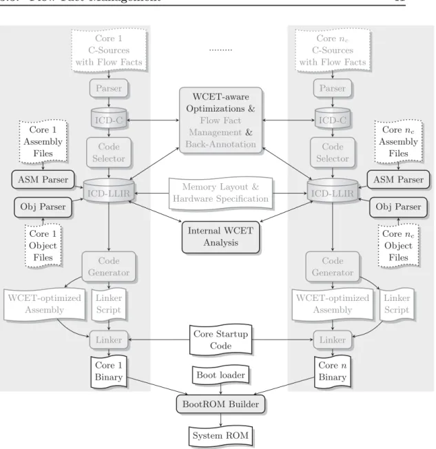
This thesis presents multiple approaches towards a precise WCET analysis for multi- cores, which may help to alleviate the aforementioned problems with the adoption of multi-core hardware in real-time system design. Also, the concrete implementation of these approaches inside the WCET-aware C Compiler (WCC) is demonstrated and used to evaluate the presented techniques. The WCC also provides unique opportunities to couple the analysis of a task’s WCET with the optimization of the latter. Therefore, this thesis also presents two optimizations which utilize this unique capability to demonstrate that an optimization of task WCETs is feasible and useful in practice.

We build our approach on the branch of WCET analysis methods which has proven to be most efficient in the past, namely on a decomposition of the WCET analysis into microarchitectural analysis and path analysis. This approach is also employed in the de-facto standard WCET analyzer aiT [Abs14a]. It consists of an abstract interpretation-based microarchitectural analysis phase, during which the best- and worst-case runtime of each basic block in the task’s control-flow graph is determined. With these values a successive path analysis can compute the shortest and longest path through the control-flow graph, whose length corresponds to the BCET and WCET, respectively.

For the single-core case, the WCET analysis methodology is reviewed. Focus is laid on how to achieve a value analysis with sufficient precision and on the modeling of microarchitectural features, since these form the basis for a precise WCET analysis of both single- and multi-core systems.

The extension of the microarchitectural modeling to include shared buses and

shared caches is discussed, and the possibility to model the behavior of time-

triggered arbiters by means of TDMA offsets is presented. These can be used to

statically capture the duration of shared resource access requests. Their true poten-

tial only unfolds when they are not applied naively, but combined with intelligent

loop unrolling techniques. Since the loop unrolling incurs a significant analysis time

8 Chapter 1. Introduction

overhead, the concepts of offset relocation and offset contexts are established to allow for a fast but also precise WCET analysis.

The timing behavior of stateful resources and non-time-triggered arbiters relies on the ordering of accesses, therefore any analysis which tries to bound this timing must safely consider all possible interleavings of potentially parallel actions. This thesis for the first time presents a structured way to explore such interleavings on the single-machine-cycle level. To avoid some part of the combinatorial explosion that is inevitable in such analyses, a timing-based pruning criterion is developed which uses the generated timing information to rule out invalid parallel system states.

The presented analysis methods are compared with respect to the achievable precision and to the overhead which is incurred by platform configurations which are routinely advertised for being more predictable and thus easier to analyze.

Finally, two compiler optimizations are given, which can be used to decrease the WCET of tasks in a multi-core system. The first is a WCET-aware multi- criteria evolutionary optimization of the schedule of shared resources. By efficiently exploring different system configurations a suitable schedule can be found for a given task set. It is also shown that this schedule is highly dependent on the given tasks, i.e., an optimal default schedule cannot be specified in general, necessitating an optimization like the one presented here.

The second optimization is a WCET-driven instruction scheduling which utilizes the close coupling of analyses and optimizations inside the WCC by using microar- chitectural analysis results to optimally place single instructions inside the tasks’

source code. The placement is done in such a way that the single shared resource accesses incur minimum access overhead, which is only possible with the help of detailed microarchitectural information.

1.3 Organization of the Thesis

The structure of the remaining parts of this thesis is as follows:

• Chapter 2 presents the existing concepts used in WCET analysis. It starts with a general review of abstract interpretation, the basic method onto which the presented WCET analysis is built. Subsequently, different approaches to WCET analysis are shown, and necessary definitions of WCET-related phe- nomena like timing compositionality and timing anomalies are given. The chapter closes with a presentation of preexisting approaches to WCET analy- sis in multi-task and multi-core systems.

• The WCC framework is introduced in Chapter 3. Starting with an overview

of the compiler infrastructure and related work on similar projects, it covers

the assumed system model and the compiler phases. Finally, extensions of

the WCC framework to incorporate binary code into WCET analysis and

optimization are presented.

1.4. Author’s Contribution to this Dissertation 9

• Chapter 4 picks up the WCET analysis concepts presented in Chapter 2 and demonstrates how these are used in the context of the WCC framework to create a WCET (and BCET) analyzer for a single-core ARM platform.

• The main contributions of this thesis are found in Chapter 5, where the methods for WCET analysis in multi-core systems are discussed. It covers TDMA offset analysis for time-triggered arbiters as well as precise analysis for less predictable architectures and an extensive evaluation.

• Chapter 6 contains the presentation of the aforementioned two compiler op- timizations tailored towards WCET optimization. It starts with the evolu- tionary shared resource schedule optimizations and then proceeds with the WCET-aware multi-core instruction scheduler. For both optimizations, eval- uation results on a large number of real-time benchmarks are given.

• Finally, Chapter 7 closes the thesis with a summary and an outlook on future work.

1.4 Author’s Contribution to this Dissertation

According to §10(2) of the “Promotionsordung der Fakultät für Informatik der Tech- nischen Universität Dortmund vom 29. August 2011”, a dissertation within the context of doctoral studies has to contain a separate list that highlights the au- thor’s contributions to research and results obtained in cooperation with other re- searchers. Therefore, the following overview lists the contribution of the author on the presented results for each chapter:

• Chapter 2: This chapter summarizes related work only, therefore there is no contribution to account for.

• Chapter 3: The WCC framework [FL10] was created by a multitude of people, among others Heiko Falk, Paul Lokuciejewski, Sascha Plazar and Jan Kleinsorge. The author has also worked on this framework to some extent by using it as a basis for the multi-core WCET analysis and optimizations.

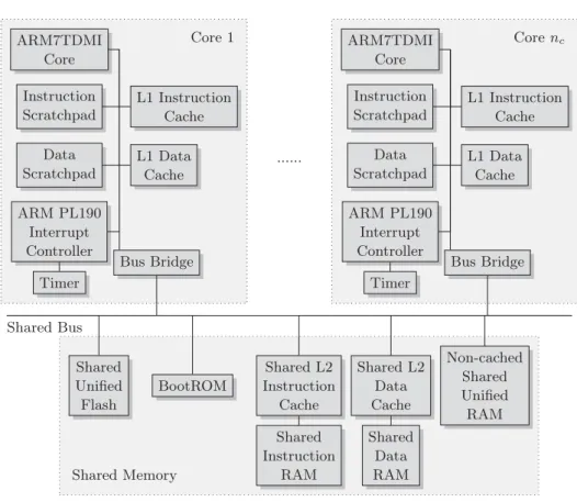
The extension of the WCC framework to multi-core architectures was done by the author only. An initial version of the virtual platform that was used to evaluate the proposed architecture was implemented by Tim Harde [Har13]

and later largely re-structured by the author. The employed cycle-true virtual platform simulator CoMET was donated by Synopsys Inc. [Syn14].

The concepts for the extension of the WCC towards the handling of binary input files were developed by the author and implemented by Christian Gün- ter [Gün13].

• Chapter 4: The WCC value analysis was developed by the author in collab-

oration with Jan Körtner, who carried out the majority of the implementation

work. The analysis and context graph handling as well as the microarchitec-

tural modeling as presented in this chapter are the work of the author.

10 Chapter 1. Introduction

• Chapter 5: The WCET analysis approaches for shared buses were entirely designed and developed by the author. They are based on previous work from Chattopadhyay et al. [CRM10], which was later extended in cooperation with the same authors in the publications [KFM+11; KFM+14]. The co-authors of these publications assisted the author in technical discussions, proof-reading and structuring of the publications. Furthermore, the presentation of the anal- yses in this thesis contains a state which is far more advanced than the one in [KFM+11; KFM+14] and integrates better with the classical microarchi- tectural analysis. These advances also are original work of the author.

The comparison of arbitration strategies as already published in [KHM+13]

was developed by the author of this thesis, based on the platform implemen- tation by Tim Harde.

The WCET analysis for stateful resources considering all possible interleavings of task executions was designed and implemented exclusively by the author and published in [KM14].

• Chapter 6: The optimization opportunities and concepts were developed and

formalized by the author. A first version of the implementation was done by

Hendrik Borghorst [Bor13] which was later reworked by the author, leading

to the publication [KMB14].

Chapter 2

Timing Analysis Concepts

Contents

2.1 Abstract Interpretation . . . . 12 2.2 WCET Analysis for Uninterrupted Single Tasks . . . . . 18 2.2.1 Static WCET Analysis . . . . 19 2.2.2 Parametric WCET analysis . . . . 21 2.2.3 Hybrid WCET analysis . . . . 21 2.2.4 Early-Stage WCET analysis . . . . 22 2.2.5 Statistical WCET analysis . . . . 22 2.2.6 WCET-friendly Hardware Design . . . . 23 2.2.7 Experiences with Practical Application of WCET Analysis 23 2.2.8 Timing Anomalies . . . . 24 2.2.9 Compositionality in WCET Analysis . . . . 27 2.3 Timing Analysis of Sequential Multi-Task Systems . . . 29 2.3.1 Accounting for the Timing Behavior of System Calls . . . . 29 2.3.2 Accounting for Task Interaction Impacts on the WCET . . 30 2.3.3 Schedulability of Multi-Task Systems with Given WCETs . 32 2.4 Timing Analysis of Parallel Multi-Task Systems . . . . . 32 2.4.1 Multi-Core Systems . . . . 33 2.4.2 Distributed Systems . . . . 34

In this chapter we will review the existing literature on WCET analysis and investigate which concepts have already been established in this domain. We start in Section 2.1 with a thorough treatment of abstract interpretation, since this is one very fundamental technique that forms the basis for WCET analysis. In Section 2.2 we examine how this technique and others can be applied in the context of classical WCET analysis. Section 2.3 proceeds with concepts for the timing analysis of multiple tasks on a single processor. Finally, we present existing approaches for the analysis of the WCET of tasks in parallel systems in Section 2.4.

11

12 Chapter 2. Timing Analysis Concepts

2.1 Abstract Interpretation

Abstract Interpretation (AI) is one of the most well-developed theories for the ap- proximation of states in discrete transition systems. The basic ideas date back to a 1973 publication from Kildall [Kil73] which were later formalized and general- ized by Cousot and Cousot [CC77]. The presentation in this thesis is based on the more modern introduction in [ALS+07]. Though AI is applicable to various discrete transitions systems like, e.g., source-code programs, petri nets and Kahn process networks, we base our examples on the approximation of low-level computer system states since these will be the target of WCET analysis.

In general, we can associate a concrete semantics with any computer system.

This semantics reflects the transformation of all memory cells in the system by operations carried out by the computational circuits. Since all currently relevant computer systems are working in clocked operation, we can define these transfor- mations on discrete time steps. Therefore, if L ˜ is the set of all possible memory cell assignments including all registers, the program counter, current instruction and otherwise stored values, a single cycle of a computer system’s operation can be deterministically described by a concrete semantics function ⟦⟧ conc ∶ L ˜ ↦ L. Since ˜ all relevant computer systems are also working on a well-defined instruction set, concrete states are always generated by programs.

Definition 1. A program X = ( i ₀ , i ₁ , . . . , i _n ) is a sequence of instructions i ∈ I from a global instruction set I with start instruction i ₀ and a set of terminal instructions I t . An execution of X is a trace of concrete system states ( ˜ l ₀ , ˜ l ₁ , . . . , ˜ l m ) such that

• ˜ l ₀ encodes X in its memory content and executes i ₀ , and

• ∀ i ∈ {1 , m } ∶ ˜ l _i = ⟦ ˜ l _{i −1} ⟧ conc , and

• pc ( ˜ l _m ) ∈ I _t .

where pc ∶ L ˜ → I extracts the value of the program counter from a concrete state.

An ideal analysis would determine the execution trace for every possible initial system state ˜ l ₀ . The length of the longest of these traces would be the WCET of the program under analysis. Obviously, a naive attempt to collect all of these traces and return them as the analysis result will fail, since

a) there may be traces of infinite length corresponding to non-terminating pro- grams and

b) modeling the whole state of the system under analysis and maintaining huge numbers of these states during the analysis is practically infeasible.

To be able to reason about program executions in a structured way, the notion of a control-flow graph is used.

Definition 2. A basic block v = ( i ^v ₀ , . . . , i ^v _k ) of a program X is a maximal sub- sequence of X, such that for all j ∈ {1 , . . . , k } and ˜ l, l ˜ ^′ ∈ L ˜

( pc ( ˜ l ) = i ^v _j ∧ ⟦ ˜ l ^′ ⟧ conc = ˜ l ) ⇒ ( pc ( ˜ l ^′ ) = i ^v _j ∨ pc ( ˜ l ^′ ) = i ^v _{j −1} ) . (2.1)

2.1. Abstract Interpretation 13

A Control Flow Graph (CFG) ( V, E, v ₀ ) of a program X, with V being the set of basic blocks of X and E ⊂ V × V being a set of directed edges which model every possible transfer of control within the program. The entry point of the program is given by node v ₀ .

A path P in a CFG from v s ∈ V to v e ∈ V is a non-empty sequence of nodes P = ( v _s , . . . , v _e ) such that for any two adjacent v _i and v _{i +1} in P , ( v _i , v _{i +1} ) ∈ E holds.

If a path from v _s ∈ V to v _e ∈ V exists, we call v _e reachable from v _s which is expressed as v s ↝ v e , else v e is unreachable from v s written as v s ↝̸ v e . The set of all paths from v _s to v _e is called P _{[ v}

_,v

_] . For any node v ∈ V , δ ⁺ ( v ) = { w ∣ ( v, w ) ∈ E } and δ ⁻ ( v ) = { w ∣ ( w, v ) ∈ E } are the successors and predecessors of v .

The connection between traces of concrete states and the CFG is easily made, since each ˜ l ∈ L ˜ holds a concrete value of the Program Counter (PC) register of the underlying architecture, which points to an instruction i _{˜ l} ∈ I . Thus, if each ˜ l _j of a trace is mapped to the node v ∈ V with i _{˜ l}

j

∈ v the trace is transformed to a CFG path.

A path is called feasible, if there is a concrete trace which is mapped to this path. Infeasible paths may exist in a CFG due to dependencies between control flow branches, which are not reflected in the graph structure. As an example, if two branches b ₁ and b ₂ have the same branch condition and the value of the condition remains unmodified between b ₁ and b ₂ , then either both branches are taken or none.

The CFG, in contrast, may also contain an infeasible path in which b ₁ is taken whereas b ₂ is not. A cycle at v ∈ V is a path ( v, . . . , v ). A path which contains no cycle is called acyclic. The set of all paths P _{[ v}

_,v

_] can be restricted to feasible (P _[ ^feasible _v

_,v

_] ) or acyclic paths (P _[ ^acyclic _v

s

,v

] ).

To deal with issue a) from above, the collecting semantics ⟦⟧ coll ∶ 2 ^{L ˜} × V ↦ 2 ^{L ˜} is defined as taking a set of concrete states, executing the instructions from the given CFG node in those states for all possible inputs and returning the resulting end states. We can trivially extend the collecting semantics to paths p = ( v ₁ , v ₂ , . . . v _n ) by setting ⟦ s ⟧ ( p ) = ⟦ . . . ⟦⟦ s ⟧ ( v ₁ )⟧ ( v ₂ ) . . . ⟧ ( v _n ) . We are then searching for the state set s ^coll _v = ⋃ p ∈ P

0,v]

,˜ l

∈ L ˜ ⟦ ˜ l ₀ ⟧ ( p ) for every node v ∈ V . If L ˜ has infinite cardinality, this result may still be infinitely big. To overcome this and the issue b) mentioned above, AI further changes from the collecting semantics ⟦⟧ coll to an abstract semantics

⟦⟧ abs ∶ L × V ↦ L which is defined on abstract system states L. To be useful, the abstract semantics must overapproximate the collecting one, which is expressed by the notion of a Galois connection.

Definition 3. A Galois connection ( α, γ ) is a pair of functions α ∶ P ↦ Q and γ ∶ Q ↦ P for two sets with partial orders ( P, ≤) and ( Q, ⊑) such that

∀ x ∈ P, y ∈ Q ∶ α ( x ) ⊑ y ⇔ x ≤ γ ( y ) (2.2)

For our concrete example, this means ( P, ≤) = (2 ^{L ˜} , ⊆) and ( Q, ⊑) = (L , ⊑), where

x ⊑ y if and only if γ ( x ) ⊆ γ ( y ) . I.e., an abstract state x is “bigger” than y if and

14 Chapter 2. Timing Analysis Concepts

2 ^{L ˜} 2 ^{L ˜}

L L

α

⟦⟧ coll

⟦⟧ abs

γ

Figure 2.1: The Galois connection between concrete and abstract semantics.

only if it “contains” a superset of the concrete states which are contained in y. This is a general necessity in a Galois connection, where we also have the property, that x ≤ γ ○ α ( x ) , e.g., the re-concretization of an abstraction of x always contains x.

The general idea is visualized in Figure 2.1. With the abstraction function α, we can map the initial system states into the abstract domain L, where we conduct our analyses to compute abstract results l _v ^out . After the analysis is finished the Galois condition ensures that γ ( l ^out _v ) ⊇ s ^coll _v , i.e., every reachable concrete state is covered in the result. Since we are computing an overapproximation, potentially also other states which are not reachable in any concrete execution are covered.

For the analysis to be efficiently possible, the abstract domain L must be a semi-lattice.

Definition 4. A semi-lattice (L , ⊔) is a set L with a meet operator ⊔ ∶ L ↦ L , which is required to be

• idempotent: ∀ l ∈ L ∶ l ⊔ l = l,

• commutative: ∀ l, m ∈ L ∶ l ⊔ m = m ⊔ l and

• associative: ∀ l, m, n ∈ L ∶ l ⊔ ( m ⊔ n ) = ( l ⊔ m ) ⊔ n.

The meet operator induces a partial order ⊑ on L , which is defined by

∀ l, m ∈ L ∶ l ⊑ m ⇔ l ⊔ m = m (2.3) In a semi-lattice (L , ⊔) , also a biggest element ⊺ = ⊔ L exists, with ∀ l ∈ L ∶ l ⊔ ⊺ = ⊺ or equivalently ∀ l ∈ L ∶ l ⊑ ⊺ . This element is usually named “top”. Additionally, a smallest element ∈ L (“bottom”) may exist, with ∀ m ∈ L ∶ ⊔ l = l.

The height of a lattice is one less than the length of the longest sequence ( l ₁ , l ₂ , . . . , l _n ) of l _i ∈ L such that ∀ i ∶ l _i ⊑ l _{i +1} .

Definition 5. A monotonic Data-Flow Analysis (DFA) framework ((L , ⊔) , F ) con- sists of a

• semi-lattice (L , ⊔) and

• a set F containing functions f ∶ L → L , where

1. every f is monotonic in ⊑ , i.e., ∀ l, m ∈ L ∶ l ⊑ m ⇒ f ( l ) ⊑ f ( m ) ,

2. the identity function id with ∀ l ∈ L ∶ id ( l ) = l is contained in F and

2.1. Abstract Interpretation 15

3. F is closed under function composition, i.e., ∀ f, g ∈ F ∶ f ○ g ∈ F . A DFA framework is called distributive iff

∀ f ∈ F, l, m ∈ L ∶ f ( l ⊔ m ) = f ( l ) ⊔ f ( m ) (2.4) The weaker form of this condition f ( l ⊔ m ) ⊑ f ( l ) ⊔ f ( m ) is already true also for non-distributive DFA frameworks.

Definition 6. An instance of a DFA framework ((L , ⊔) , F ) is a tuple (( V, E ) , v ₀ , l ₀ ) , where ( V, E ) is a control-flow graph of the program to analyze, v ₀ is the node where the control flow enters the program and l ₀ ∈ L is the initial data-flow information for the start node and every node v ∈ V has an associated transfer function f v ∈ F.

A solution for an instance is a set of data-flow items l ^out _v for all v ∈ V such that the reachable concrete states s ^coll _v are covered, i.e., γ ( l ^out _v ) ⊇ s ^coll _v .

The transfer functions are just invocations of the abstract semantics, i.e. f v =

⟦⟧ abs ( v ) and similar to it, we can extend the transfer function to CFG paths. By following all feasible paths through the program’s control flow graph given by a DFA framework instance, we can define an ideal solution

l _v ^out,IDEAL = ⊔

p ∈ P

0,v]

f _p ( l ₀ ) (2.5)

Since the identification of feasible paths in impossible in general, we can relax this to the Meet Over All Paths (MOP) solution, which considers all paths in the CFG

l _v ^out,MOP = ⊔

p ∈ P

f _p ( l ₀ ) (2.6)

The MOP solution is still not computable, since there may be infinitely many paths due to the existence of loops in the CFG as already discussed. Therefore as the last coarsening step, we revert to the Minimum Fixed Point (MFP) solution which is the fixed point of Equation 2.7.

l ^out,MFP _v = ⎧⎪⎪

⎨⎪⎪ ⎩

f _v ( l ₀ ) if v = v ₀

f _v (⊔ ( u,v )∈ E l ^out,MFP _u ) else (2.7) This solution avoids the computation of all paths by only propagating the states via the edges of the CFG until a fixed point is reached. During this procedure all finite paths are visited implicitly. From the fixed point definition we also know, that for all infinite paths to v the generated data-flow information is covered by l ^out,MFP v . Further details on why the precision relation l _v ^out,MFP ⊒ l ^out,MOP _v ⊒ l ^out,IDEAL _v is true for all v ∈ V can be found in [ALS+07, Chapter 9.3].

For monotonic frameworks, an MFP solution always exists according to the

Knaster-Tarski-Fixed-Point Theorem [Tar55]. In general, the MOP solution is more

precise than the MFP one, since in the MFP case we apply the meet operator

16 Chapter 2. Timing Analysis Concepts

Algorithm 1 The generic data-flow analysis work-list algorithm.

1: function WorkListAlgorithm (((L , ⊑) , F ), (( V, E ) , v ₀ , l ₀ ))

2: worklist ← v ₀

3: for v ∈ V do ▷ Initialization of the l _v ⁱⁿ /l _v ^out ...

4: if v = v ₀ then

5: l ⁱⁿ _v ← l ₀ , l ^out _v ← ▷ ... for the start node ...

6: else

7: l ⁱⁿ _v ← , l ^out _v ← ▷ ... and for all other nodes.

8: while worklist ≠ ∅ do ▷ Loop until a fixed point was found

9: v ← pop(worklist)

10: l ⁱⁿ _v ← ⊔ ( u,v )∈ E l ^out _u

11: l ^tmp _v ← f _v ( l _v ⁱⁿ ) ▷ Apply transfer function of node v

12: if l _v ^out ≠ l _v ^tmp then ▷ If there were changes at node v ...

13: l ^out _v ← l ^tmp v

14: for ( v, w ) ∈ E do

15: push(worklist , w ) ▷ ... propagate them to all successors

16: return { v → l ⁱⁿ _v ∣ v ∈ V }

earlier than in the MOP case, namely after each node instead of only after each path. For distributive frameworks this does not make a difference (see Equation 2.4), therefore the MFP solution is equal to the MOP solution for distributive frameworks (“Interprocedural Coincidence Theorem” [KS92]). For computing the MFP solution, the work-list algorithm is a standard approach as shown in Algorithm 1.

The data-flow information is initialized in lines 3-7 and then propagated through the graph in lines 8-15. The nodes at which the data-flow information has not yet converged are kept in a work-list which is processed until all state information has converged. As mentioned, this convergence relies on the monotonicity of the height of the underlying lattice. For finite-height lattices, the convergence is guaranteed, since any data-flow item either reaches a fixed point other than ⊺, or reaches ⊺ in a finite number of steps which is a forced fixed point due to the monotonicity of the transfer functions. To speed up the convergence of the data-flow items we can sort the work list in topological order, ignoring back-edges in the CFG.

As an example for a lattice, consider the problem of determining whether a single register has a constant value at the individual CFG nodes. The Hasse diagram of the lattice for this problem is shown in Figure 2.2. It has a finite height of 2 , though it has an infinite number of elements. The bottom element denotes the state “register was not initialized”, the top state ⊺ means “register does not hold a constant value”

and the middle row of elements represents actual constants. Whenever a block v

loads a constant value into the register, l ^out _v is set to this value. If multiple constants

are merged in the meet operation, l ⁱⁿ _v is set to ⊺ in Algorithm 1. Further examples

and an overview of possible lattices for program analysis can be found in [Cou01].

2.1. Abstract Interpretation 17

⊺

−∞ . . . −2 −1 0 1 2 . . . ∞

Figure 2.2: The lattice of integer constants.

Since the convergence of Algorithm 1 is not guaranteed for lattices with infi- nite height, such as intervals on integer numbers, widening is used to enforce the termination of the abstract interpretation in such lattices.

Definition 7. A widening operator Δ is a unary function on L , such that ∀ l ∈ L ∶ l ⊑ Δ ( l ) and for any sequence l ₁ , l ₂ , . . . with ∀ i > 1 ∶ l _i ⊐ Δ ( l _{i −1} ) the top element is reached in a finite number of steps, i.e., l n = ⊺ for some n ∈ N .

With a widening installed, line 11 in Algorithm 1 becomes l ^tmp _v ← Δ ( f _v ( l ⁱⁿ _v ))

After the fixed point was found, it is possible to refine the results again by letting the main loop of Algorithm 1 iterate again for a user-defined number of times with the original definition of l ^tmp v , i.e., without the widening. This process may remove some of the overestimation induced by the widening and is called narrowing. In Figure 2.3 an example is given, how widening and narrowing affects the generated results. The figures show the Hasse diagram of the lattice and the evolution of a single data-flow value (one l _v ^out for a fixed node v) during the runtime of the fixed point determination. Every arc corresponds to one iteration of the main loop from Algorithm 1 for v. The widening skips over many intermediate values by artificially coarsening the results of the individual steps. This speeds up the convergence (re- duced number of arcs) but also leads a more imprecise result (higher in the Hasse diagram). The narrowing is able to re-gain some precision by applying the unmod- ified transfer functions to the fixed point values. It can lead to results which are at best as good as in the case without widening, but usually they are worse.

To further refine the results of the data-flow analysis, path-awareness can be

introduced as shown in [HT98], which inflates the analysis lattice by multiplying

it with a lattice that represents some of the edges that were visited during the

generation of a data-flow information item. If that is done, data-flow items with

different path expressions are not merged, which potentially increases the precision

if the original lattice was not distributive. In addition, path-awareness can be used

to rule out infeasible paths [NKJ10] if the edges in the path have contradictory

guard conditions, thus moving the fixed-point result a step closer to the IDEAL

solution sketched above. All of this comes at the price of increased analysis duration,

since the size of the underlying lattice is multiplied by the number of possible edge

18 Chapter 2. Timing Analysis Concepts

⊺

(a) Without widening

⊺

(b) With widening

⊺

(c) With widening and nar- rowing

Figure 2.3: Convergence behavior in a lattice. Solid and dotted arcs represent one or indefinitely many applications of the transfer function, respectively.

strings. Therefore, [NKJ10] try to limit the edge strings to relevant edges only, heuristically. Another approach to control the complexity of the path-awareness is to gradually increase the allowed length of the path expressions during the analysis as shown in [DDY06], where the authors use this method to analyze large real-world benchmarks. As a last option, [BSI+08] separate the detection of infeasible paths from the data-flow analysis itself and re-structure the program such that infeasible paths are avoided also in a non-path-aware analysis.

With the systematical description of a DFA framework coined above, it should not be surprising that DFA implementations for concrete problems can easily be generated from compact lattice and transfer function descriptions [SSB09], even for path-aware DFAs [HMM12].

2.2 WCET Analysis for Uninterrupted Single Tasks

In this section we will review the existing approaches to the determination of WCET estimates for a single program running without interruption on a single-core com- puter with no other active hardware components which could interfere with the program under analysis. This is the most basic of all WCET analysis scenarios, but it already offers a plethora of pitfalls and problems to solve [WEE+08]. In general, the challenges that WCET analysis is facing in this scenario fall into one of the following categories:

• Unpredictable hardware components: The WCET analysis has to follow all execution paths of the hardware to find the path with maximum execution time. Abstract interpretation can relieve this problem to some limited ex- tent, but strong abstractions on the hardware state also lose much precision.

Therefore, hardware features which increase the state space of the pipeline

or memory hierarchy such as caches, superscalar and out-of-order execution,

2.2. WCET Analysis for Uninterrupted Single Tasks 19

Program Code

User Annotations CFG

Reconstruction

Value Analysis

Microarchitectural Analysis

Path Analysis

WCET Figure 2.4: Structure of most static WCET analyzers.

fetch and commit queues and speculative execution complicate the WCET analysis [WGR+09].

• Unpredictable software structure: Usage of runtime-dynamic software constructs like function pointers, virtual inheritance and even dynamic mem- ory allocation is hard to analyze statically. These can be circumvented to some extent by coding conventions such as MISRA-C [MIS13] which prohibit the usage of these features. Nevertheless even predictably-designed software exhibits an iteration structure of loops and recursions which may be not ana- lyzable statically. Here, the user has to intervene in the worst case and needs to give hints to the WCET analyzer [KKP+11].

The following subsections will introduce the important branches of single-task WCET analysis, review real-life examples and case studies of their application and finally finish with an introduction to timing anomalies and compositionality, two concepts which are central to WCET analysis and frequently used in the following sections.

2.2.1 Static WCET Analysis

Static WCET analysis analyzes a program without executing any part of it, solely based on abstract models of the hardware and program semantics. Therefore, it provides stronger safety and coverage guarantees than measurement-based methods.

The usual approach is to separate the analysis into multiple steps as shown in Figure 2.4.

A program, which, depending on the analyzer, may be given in binary or source-

code form, is first fed into the control-flow graph reconstruction which extracts an

interprocedural control-flow graph that reflects all possible transitions of control flow

among instructions from the given program. In case of non-analyzable control-flow

transitions, such as function pointers, the user might be required to specify their

targets manually. After this step, the value analysis computes safe approximations

of the register or variable values by means of AI on the generated CFG. The user can

manually refine these results if he is not satisfied with their precision. The microar-

chitectural analysis uses the CFG and the value results to provide overestimates of