Modelling with Partial Differential Equations
Many practical applications involve the description of the state of a solid body, a fluid (in continuum mechanics no distinction is made between fluids and gases) or just any region of space. As examples consider the gravity field of an inhomogeneous body, the temperature of a solid body, the flow of water in the subsurface, the flow of gases in a complicated duct, the propagation of sound or water waves or the mechanical stress in a bridge. In this chapter, we will derive the equations of mathematical physics that describe all these phenomena.
1.1. Gravitation
Newton’s famous law of gravitation
F(x,y) =G mM
�y−x�2 y−x
�y−x� (x�=y) (1.1)
gives the force vector acting on a point mass m at positionx∈ R3 excerted by another point mass M located at a pointy ∈ R3 and G is the gravitational constant with the approximate value 6.67·10−11 N m2 kg−2(there is some debate about the value – it is difficult to measure).
Newton’s law is stated for point masses as it has first been applied to the sun and the planets in the solar system. But how does it act in a cloud of gas of varying density? Since there are so many atoms (or molecules) in the gas it would be overwhelmingly expensive to compute all the forces (O(N2)effort forN particles).
We now wish to derive a new form of Newton’s law in the form of a PDE that is usable in this case. First we rewrite Newton’s law a little bit by introducing the function
ψ(x,y) = − GM
�y−x� (1.2)
which is called the gravitationalpotential of a point mass in physics. In mathematics 1/�y−x� is calledsingularity function. It has the following interesting properties:
∇xψ(x,y) = −GM(y−x)
�y−x�3 , ∆xψ(x,y) =
�3
i=1
∂2x2
iψ(x,y) =0 (x�=y).
Using it we can rewrite Newton’s law as
F(x,y) =ma(x,y), a(x,y) = −∇xψ(x,y).
Note that the acceleration a(x,y)is independent of the massm (equivalence principle).
Now consider an arbitrary domainω⊂R3(open and connected set of points) with sufficiently smooth boundary∂Ω, a pointy�∈∂ω and compute the
�
∂ω
a(x,y)·n(x)dsx= −
�
∂ω∇xψ(x,y)·n(x)dsx (1.3) wheren(x) denotes the exterior unit outer normal vector to ω. By dsx we indicate that the surface integral is done with respect to the variable x and not y. For the evaluation of the integral we need to consider two cases:
i) y�∈ω. By applying Gauss’ integral theorem �
ω∇ ·u dx=�
∂ωu·n dswe get
−
�
∂ω∇xψ(x,y)·n(x)dsx = −
�
ω
∆xψ(x,y)dx=0 since∆xψ(x,y) =0 for any x∈ω sincey is outsideω.
ii) y∈ ω. Now the trick from case I can not be done so easily becauseψ has a singularity forx=ybut it can be modified. Let B�(y) ={x∈R3 : �x−y�< �}be the open ball of radius�aroundy. Then again applying Gauss’ theorem we get
0=
�
ω\B�(y)
∆xψ(x,y)dx=
�
∂ω∇xψ(x,y)·n(x)dsx−
�
∂B�(y)∇xψ(x,y)·n(x)dsx
The left hand side integral is zero and the minus sign is due to the fact the normal to ω\B�(y)points into the ball B�(y). The second integral on the right hand side can be computed directly as �
∂B�(y)∇xψ(x,y)·n(x)dsx =4πGM independent of�.
So we get the following result:
�
∂ω
a(x,y)·n(x)dsx =
� −4πGM y∈ω
0 else . (1.4)
Now we extend this to a distributed mass by introducing the density function ρ : R3 → R with units kg m−3. For any domain ω⊂R3 then Mω=�
ωρ dxgives the mass contained in ω. We further assume that the density distribution is such that the integral �
R3ρ dx exists.
Then the acceleration experienced at a point x excerted by the mass distribution ρ can be computed by subdividing the mass into an infinite number of infinitesimal piecesViat position yi (superposition principle):
a(x) = lim
N→∞
�N i=1
Gρ(yi)Vi∇x
� 1
�y−x�
�
=G
�
R3ρ(y)∇x
� 1
�y−x�
�
dy. (1.5) One can check that this integral is well defined despite the singularity, i.e. it holds also for a pointxinside a body with mass distribution ρ(transform to spherical coordinates aroundx).
Now being very careful with evaluating integrals one finds that for this acceleration and any
suitable ω⊂R3 �
∂ω
a(x)·n(x)ds= −4πG�
ω
ρ(x)dx
(only the mass insideωplays a role). Applying again Gauss’ theorem on the left hand side we
find �
ω∇ ·a(x)dx= −4πG
�
ω
ρ(x)dx.
If ais sufficiently smooth the fact that ω can be chosen arbitrarily implies that the equality also holds for the integrands themselves (see e.g. [Smirnow, 1981, § 74]) and we arrive at
∇ ·a(x) = −4πGρ(x) (x∈R3). (1.6) The final piece is the observation that all fundamental forces in nature are conservative (a basic principle that is assumed to hold by physicists). In a conservative force field the path integral w(a,b) = �b
aF(s)·t(s)ds (t is the unit tangential vector) does only depend on the points a,b but not on the particular path taken from a to b. Conservativity of the force is a consequence of conservation of energy because otherwise it would be possible to generate energy in a force field by taking different paths back and forth. With an arbitray reference point r0 we then have w(a,b) = w(a,r0) +w(r0,b) = w(r0,b) −w(r0,a) = w�(b) −w�(a) where w�(x) =w(r0,x)is now only a function with a single argument, called thegravitational potential. Invoking the main theorem of calculus in its multi-dimensional form
�b
a∇Ψ(s)·t(s)ds=Ψ(b) −Ψ(a) (1.7) we see that a force is conservative if and only if it can be represented as the gradient of a potential. The potential is only unique up to a constant as can be seen from (1.7).
Sincema(x) with a(x) from (1.6) is the gravitational force experienced by a point massm at positionx and the gravitational force is supposed to be conservative we conclude that there must exist a scalar functionΨ(x)such thata(x) = −∇Ψ(x). Inserting this into (1.6) we obtain
∇ · ∇Ψ(x) =∆Ψ(x) =4πGρ(x) (x∈R3). (1.8) This equation is called Poisson equation. As stated Ψ is assumed to be twice continuously differentiable, which requires ρ to be at least continuous. This is practically very restrictive since, for example, the density function of the moon (having no atmosphere) might be very well approximated by a discontinuous function. It is an important part of PDE theory to give equation (1.8) a precise mathematical meaning also in this sense. The potential is determined by Equation (1.8) up to a constant. To fix the constant, an additional condition for the behaviour ofΨforx→∞can be imposed.
1.2. Fluid Mechanics
1.2.1. Continuum Hypothesis and Scales
Materials such as solids or fluids are made up of atoms or molecules with void space in between (we do not consider quantum effects, although, also there, partial differential equations do play
a role). Practical problems often involve excessively large numbers of atoms as we are interested in the behaviour of the material on a length scale that is very large compared to the average distance of the atoms. We call this scale of interest the macroscopic scale and the scale of the discrete particles the microscopic scale.
In continuum mechanics, the properties of the material are assumed to be (piecewise) contin- uous (or even differentiable) functions in the mathematical sense. The discrete particles are not considered, instead macroscopic properties (e.g. velocity) are defined as appropriate averages of the microscopic properties. By averaging, new quantities (such as density, temperature or pressure) arise that have no equivalent on the microscopic scale. The validity of this continuum hypothesis depends on the number of atoms (so that averages are representative) and whether the micro- and macroscale are sufficiently separated (a property called scale separation).
The laws on the microscale give now rise to new (effective) laws on the macroscale that connect the macroscopic variables. Current research is very much interested in so-called multi- scale problems where the effective macroscopic laws (or coefficients in these laws) are not easily determined from the micoscopic scale (such as porous medium problems) or where there is no scale separation (e.g. turbulence).
In this chapter, fluids are considered while in the next chapter the deformation of elastic solid bodies is considered.
1.2.2. Conservation Principle
Conservation of mass, linear and angular momentum as well as energy are basic empirical law of physics (throughout this text we consider only classical mechanics where mass and energy are distinct quantities). Conservation states that the total amount of such an extensive state variable in a closed system remains constant over time. In an open system, the total amount of the quantity can vary through exchange with the environment. We are now about to state the principle of conservation in mathematical form.
ω Ω
We consider a compressible fluid material that fills a domain Ω ⊆ Rn, n = 1, 2, 3, which is open and connected. The domain ω ⊂ Ω is chosen arbitrarily within Ω (see figure). For the subsequent derivation,ωandΩare fixed in space and do not depend on time (an assumption to be relaxed when solids are considered). The function ρ(x,t)gives the mass density in units1 kg m−3 for any pointx∈Ω at timet(other units, such as mol m−3 may be appropriate depending on the problem). The total massMω(t)(in kg) contained in ωat time t is then given by
Mω(t) =
�
ω
ρ(x,t)dx.
The principle of conservation now states that over time the mass in ω can change only due to flow of material over the boundary∂ωor due to injection or extraction of material into or fromω. To formulate this precisely, the velocity of the materialv(x,t)in m s−1 and the source functionf(x,t) in kg m−3 is given. For an arbitrary time interval,∆tthe we can state:
Mω(t+∆t) −Mω(t) =
�t+∆t
t
��
ω
f(x,r)dx−
�
∂ω
ρ(x,r)v(x,r)·n(x)ds
�
dr . (1.9)
1We always state units in the MKS (meter kilogram second) system.
The volume integral gives the contribution from sources and sinks withf >0 denoting a source andf <0 denoting a sink. In the surface integral,n(x)denotes the exterior unit normal vector at x∈∂ωand thereforev·n >0 results in a reduction of the mass in ω.
Using�t+∆t
t g(r)dr=∆t g(t)+O(∆t2)for sufficiently smoothg, passing to the limit∆t→0 and applying Gauß’ theorem �
ω∇ ·u dx = �
∂ωu· n ds we obtain from (1.9) the integro- differential form of the conservation law:
∂t
�
ω
ρ(x,t)dx+
�
ω∇ ·(ρ(x,t)v(x,t))dx=
�
ω
f(x,t)dx (for anyω). (1.10) For sufficiently smooth functions, the fact that (1.10) holds for any ω implies the final differ- ential form of the mass conservation law (see e.g. [Smirnow, 1981, § 74]):
∂tρ(x,t) +∇ ·(ρ(x,r)v(x,r)) =f(x,t), x∈Ω. (1.11) If the fluid is incompressible then ρ(x,t) =const implies
∇ ·v(x,t) =f(x,t), x∈Ω (1.12)
which further reduces to ∇ ·v=0 when there are no sources and sinks present (i.e the velocity field of an incompressible fluid without sources and sinks is divergence free).
The other conserved quantities energy and momentum can be imagined as being attached to mass. In the case of energy we set e(x,t) =ρ(x,t)u(x,t), where eis the energy density with units J m−3 anduis the specific energy with units J kg−1. We can compute the energy stored in the material occupying the volume ω as
Eω(t) =
�
ω
e(x,t)dx=
�
ω
ρ(x,t)u(x,t)dx.
Repeating the reasoning given above with ρ replaced by ρu yields the energy conservation equation
∂t(ρ(x,t)u(x,t)) +∇ ·q(x,t) =f(x,t), x∈Ω, (1.13) where q(x,t) is now the energy density flux vector. If energy is simply flowing with the fluid (e.g. no conductive heat transport) we have q=ρuv.
Similarly the (linear) momentum density (having units momentum per volume) is defined as ρv. Integration over an arbitrary volumeωgives the total momentum in ω:
Pω(t) =
�
ω
ρ(x,t)v(x,t)dx.
Note however, thatP(x,t)is a vector-valued function! For each componentρvi of the momen- tum density vector we obtain the conservation equation
∂t(ρ(x,t)vi(x,t)) +∇ ·ji =fi(x,t), x∈Ω, i=1, . . . ,d,
where ji is the momentum density flux vector for the given component. If momentum is only transported with the fluid (as in inviscid flow, see § 1.2.4) we haveji=ρviv.
By defining theji to be the rows of the matrixJand defining∇ ·Jas applying the divergence to each row (yielding a vector, see § A.2.3) one can write the momentum conservation law in compact form as
∂t(ρ(x,t)v(x,t)) +∇ ·J=f(x,t), x∈Ω. (1.14) In the case of inviscid flow we then have J= ρvvT. The term ∂t(ρv) on the left hand side is rate of change of momentum density which is a force density (units N m−3). Equation (1.14) is Newton’s second law generalized to spatially extended bodies.
1.2.3. Heat Transfer
As an application of conservation laws we consider the flow of heat in a solid or fluid filling the bounded domainΩ⊂ R3. The conserved quantity is the thermal energy. Its density e is assumed to be proportional to temperature
e=ρcT
wherecis the specific heat capacity in J kg−1K−1, ρis the mass density of the material in kg m−3 and the absolute temperatureT is given in Kelvin K.
In fluids and solids the flow of thermal energy is modelled as qd = −λ∇T
which is known as Fourier’s law or diffusive flux. It states that flow is in direction of the steepest descent of temperature. The constant of proportionality is the heat conductivityλ >0 with units J s−1m−1 K−1. Heat conductivity may depend on position and time (e.g. in a fluid with varying composition).
In a fluid thermal energy is also transported with the fluid velocity v which gives rise to a convective flux
qc=ev=ρcT v.
The total flux is then the sum of convective and diffusive flux. Inserting all this into the conservation law (1.13) (now withu=cT) we obtain the convection-diffusion equation
∂t(ρcT) +∇ ·(ρcT v−λ∇T) =f in Ω (1.15) which is a scalar linear second-order PDE. In order to fully determine the temperatureT(x,t) forx∈Ωandt >0, boundary conditions
T(x,t) =g(x,t) (x∈Γ ⊆∂Ω,t >0, Dirichlet), (1.16a) (ρcT v−λ∇T)(x,t)·n(x) =j(x,t) (x∈∂Ω\Γ,t >0, Neumann) (1.16b) and the initial condition
T(x, 0) =T0(x) (x∈Ω) (1.17)
must be given.
The right hand side fwith units J s−1 m−3 of equation (1.15) models sources and sinks. In a solid this rate is usually known. In a fluid the source/sink term depends on the temperature of the fluid going in or out of the domain. It can be modelled asf=rcT whererin kg s−1m−3 is the amount of fluid entering or leaving the domain. Whenr >0 fluid (and with it thermal energy) is going in and the temperature of this fluid is known. Whenr <0 fluid is going out and the temperature of this fluid is unknown and must be computed. This leads to the final form, the so-calledconvection-diffusion-reaction equation:
∂t(ρcT) +∇ ·(ρcT v−λ∇T) +rcT =f inΩ. (1.18) Note that in this equation all coefficient functions may depend on position and time. Several important simplifications of this equation can be stated:
a) No convective flux (reaction-diffusion equation):
∂t(ρcT) −∇ ·(λ∇T) +rcT =f inΩ.
b) No diffusive flux (first-order PDE):
∂t(ρcT) +∇ ·(ρcT v) +rcT =f inΩ.
c) Stationary heat flow (all coefficients are independent of time):
∇ ·(ρcT v−λ∇T) +rcT =f inΩ.
d) Stationary heat flow in a solid:
−∇ ·(λ∇T) +rcT =f inΩ. (1.19)
e) Stationary heat flow with constant conductivity and no sinks (Poisson equation):
−∇ ·(∇T) = −∆T =f inΩ.
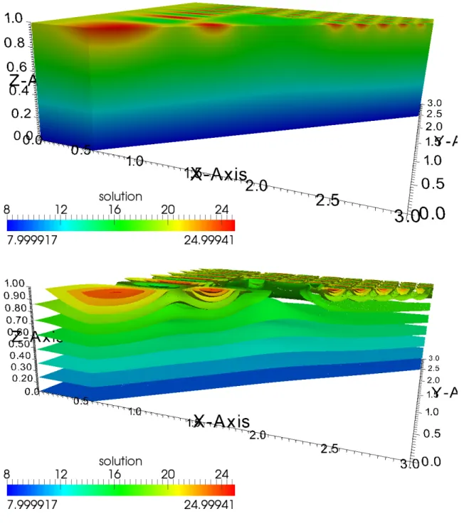
Example 1.1. Figure 1.1 illustrates the solution for a three-dimensional heat transfer problem.
The domain is Ω= (0, 3)×(0, 3)×(0, 1)and the parameters were v=0 (no convective flux), ρ = 1, c = 1, λ = 1, r = 0 and f = 0. The lateral boundaries and the region (1, 2)× (1, 2)×{1}on the top boundary were isolated, i.e.∇T·n=0, the bottom boundary was held at constant temperatureT=8 and at the remaining part of the top boundary a Dirichlet condition oscillating in space and time was given. Practically one can imagine a piece of subsurface that is heated periodically from the top and that is held at constant temperature from below. The Figure shows that the oscillations are quickly dampened by the diffusion, a fact that is also
observed in nature. �
Another important feature of the solution of the heat transfer problem without sources and sinks and divergence free velocity fieldv is that the maximum (minimum) temperature in the interior of the domainΩdoes not exceed (go below) the maximum (minimum) temperature at the boundary and initial condition. This is called a maximum principle. For details we refer to [Hackbusch, 1986] or [Evans, 2010].
Multiscale Problems
Multiscale problems are problems with highly oscillating coefficient functions. Imagine a het- erogeneous solid composed of two materials with different heat conductivity coefficient. The two materials occupy different regions of space and are arranged in a periodic fashion with periodicity�in all directions:
λ�(x) =ˆλ�x
�
�, ˆλ(x+ei) =ˆλ(x) (i=1, . . . ,n) (1.20) (ei being the ith cartesian unit vector). The 1-periodic coefficient function ˆλ taken in Ω = (0, 1)n defines the “unit cell”. Then we consider the family of stationary heat transfer problems
−∇ ·(λ�(x)∇T�) =f inΩ (1.21)
depending on the parameter � >0 together with appropriate boundary conditions.
Figure 1.1.: Solution of a 3d heat transfer problem (details given in the text).
Ω
∇T·n=0
∇T·n=0
T =1 T =1
∇T·n=0 T =0
(0, 0) (1, 0)
(0, 1)
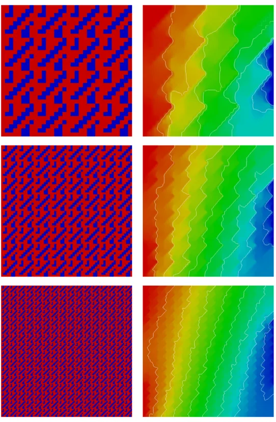
Figure 1.2.: Setup and solution for homogenous coefficient in the multiscale example.
Figure 1.3.: Conductivity distribution in the unit cell.
Figure 1.4.: Example of a multiscale problem in 2d (details given in the text).
Example 1.2. We consider an example of a multiscale problem in two space dimensions.
Figure 1.2 on the left shows the setup of the macroscopic problem and the image to the right shows the solution to this problem with a homogeneous conductivity coefficient. Now we solve a problem with the same boundary conditions and a heterogeneous periodic coefficient as defined above. The conductivity distribution in the unit cell is shown in Figure 1.3 and in Figure 1.4 the solution for � = 1/4, � = 1/8 and � = 1/16 is shown. The solutions suggest that for
�→0 the solution T� converges to a smooth function. For finite � >0 the solution has small
oscillations of the order �. �
In practical applications � � 1 and computing T� is prohibitively expensive. Moreover one is only interested in the macroscopic behaviour and not in the behaviour on the scale
�. Homogenization theory, see e.g. [Kozlov et al., 1994], shows that the limit solution T = lim�→0T� can be computed as the solution of a homogeneous heat transfer problem
−∇ ·(Λ∇T) =f in Ω
where theeffective coefficient Λ∈Rn×n is a symmetric and positive definite matrix that only depends on the conductivity distribution in the unit cell and is therefore cheap to compute.
From example 1.2 it becomes clear that the effective coefficient cannot just be a scalar as in this case the solution would be symmetric around y =1/2 as in Figure 1.2. Instead, the contour lines are tilted to the right because the material conducts better in the direction (1, 1)than in the direction(1,−1).
The discussion so far involved only two scales, the macroscopic scale of interest and the scale
� (actually there is a third scale, the atomistic scale that has has already been eliminated by deriving the heat transfer equation). In practice, there might be more than two scales involved.
For an effective solution it is important that the macroscopic scale of interest and the small scales (one is not really interested in) are clearly separated.
Another situation arises when the precise arrangenment of the materials is unknown, as is often the case with natural materials (such as e.g. rock). Then a stochastic approach may be appropriate leading to the field of stochastic partial differential equations.
1.2.4. Inviscid Fluid Flow
The flow of a gas is a very interesting and important problem. It has applications e.g.in weather and climate prediction or in star formation and the development of galaxies in astronomy.
Figure 1.5 shows an image of the Cone Nebula in the galaxy NGC 2264 which is just a pillar of gas and dust. It is supposed to be a region where new stars are formed. In this section, we consider the flow of a gas ignoring the effect of internal friction. Besides the conserved quantities density, linear momentum and energy an additional concept is needed to derive the governing equations.
Pressure
In a gas that is macroscopically at rest the molecules still perform a random motion at the microscopic level. The molecules hitting the walls of the container excert a macroscopic force that must be counterbalanced by the rigid wall. This force per unit area is called pressure with units N m−2. Through experiment one finds that the force per unit area excerted by the gas (at constant pressure) is always the same regardless of the shape of the wall. Therefore, the
Figure 1.5.: Cone Nebula (NASA/ESA image taken with the Hubble Space Telescope. For more information seehttp://www.spacetelescope.org/images/heic0206c/).
(scalar) pressure is the magnitude of a force (per unit area) that acts always perpendicular to the wall of the container (i.e. in the exterior normal direction).
If we would suddenly introduce a new (infinitely thin) wall inside the container (imagine a test volumeω) a force (per unit area) would be exerted at every point from each side of the wall that has equal magnitude and opposite direction so that it cancels out. We can therefore imagine pressure to be a (scalar) quantity that is defined everywhere in the gas.
The effect of pressure (being a force per unit area) needs to be considered in the momentum balance equation (1.14). If we consider a small test volume ω then the total force (including the direction) acting on the surface is given by
−
�
∂ω
pn ds= −
�
ω∇ ·(pI)dx= −
�
ω∇p dx. (1.22)
This term is part of the right hand side of the integral version of equation (1.14) andIdenotes the identity matrix. Note how the force always acts in negative normal direction. The sign can be understood as follows. Imagine the test volume to be a cuboid and consider e.g. thex- direction with the two faces located atx1,x2withx1< x2and corresponding normal directions n1 = (−1, 0, 0)T and n2 = (1, 0, 0)T. Then x- momentum must increase when pressure acts at the face atx1 and it must decrease when pressure acts at the face atx2. Note also, that equal pressure atx1 andx2does have a zero net effect for thex-momentum in the test volume (so it is pressure difference that does have an effect).
The pressure contribution is sometimes called an interior force to distinguish it from exterior forces (such as e.g. gravity) which are only present in open systems.
Energy
In a macroscopic body of gas the total energy consists of two different forms of energy, the internal energy (translation, rotation and vibration of the molecules on the microscopic level) and the macroscopic kinetic energy due to the movement of the fluid that is macroscopically observed. Using the concept of densities we write this as
e=ρu+ρ�v�2/2 (1.23)
withethe total energy density in J m−3anduthe specific internal energy in J kg−1. According to the theory of gases an algebraic relation, called an “equation of state” (depending on the type of gas), of the form
u=u(ρ,p) (1.24)
relating specific internal energy, density and pressure can be derived. A well-known example is the ideal gas lawp=RρT¯ (here the internal energy is proportional to temperature). See below for another popular example.
Total energyeis a conserved quantity that is transported with the fluid with a fluxq=ev.
On the right hand side of the energy balance equation (1.13) internal work done in the fluid has to be considered. This internal work is known as “volume changing work” and can be experienced when using a bicycle pump: when a gas is compressed (i.e. its volume is decreased), it heats up.
ω(t) ω(t+∆t)
We can derive the expression for volume changing work as follows:
Imagine a set of molecules occupying the volume ω(t) at time t (see figure to the right). The same particles are contained in ω(t+∆t) ⊂ ω(t) at small time interval ∆t later. Subdividing ∂ω(t) into small surface elements ∆si the work done against pressure of the gas in the time interval∆tis to first order
∆Wω(t) = − lim
N→∞
�N i=1
p(xi,t)dsi
� �� �
normal force
v(xi)·ni∆t
� �� �
distance
= −∆t
�
∂ω(t)
pv·n ds= −∆t
�
ω(t)
∇ ·(pv)dx.
The sign is chosen such that compression (v·n <0) results in a positive value.
Euler Equations
Considering the internal forces due to pressure in the momentum balance law and the vol- ume change work in the energy balance law we obtain the famous nonlinear system of partial differential equations known as the Euler equations of gas dynamics in conservative form
∂tρ+∇ ·(ρv) =m, (1.25a)
∂t(ρv) +∇ ·(ρvvT +pI) =f, (1.25b)
∂te+∇ ·((e+p)v) =w, (1.25c) which together with the thermodynamical relation
p=p(ρ,e) = (γ−1)(e−ρ�v�2/2) (1.26)
and appropriate boundary and initial conditions describe the flow of a polytropic ideal gas.
The functions m, f and w denote the mass source term, the external forces and the energy source term. Equation (1.26) is a consequence of the equation of stateu=p/((γ−1)ρ)and the definition of total energy (1.23). The constantγis the adiabatic exponent and depends on the type of gas. For more details, see [Leveque, 2002, § 14.4]. Pressure is considered a dependent variable in (1.25) which can be eliminated using (1.26) resulting in a system of five equations for the five unknown functions ρ, v1, v2, v3 and ein three space dimensions. It is interesting to note that we can combine all the equations (1.25) into a single equation for the unknown vector functionw= (ρ,ρv,e)T:
∂tw+∇ ·F(w) =g (1.27)
with
F(w) =
ρv1 ρv2 ρv3
ρv1v1+p(ρ,e) ρv1v2 ρv1v3 ρv2v1 ρv2v2+p(ρ,e) ρv2v3
ρv3v1 ρv3v2 ρv3v3+p(ρ,e) (e+p(ρ,e))v1 (e+p(ρ,e))v2 (e+p(ρ,e))v3
. (1.28)
An equation of the general form (1.27) is called a (nonlinear) conservation law. Yet another often encountered form is obtained by writing out the divergence:
∂tw+
�n j=1
∂xiFj(w) =g (1.29)
where Fj(w) is the j-th column of F(w). Various other forms of the Euler equations can be found in the literature, most notably the nonconservative formulation. But (1.25) is the most general form that is also valid e.g. in the case of strong density contrasts.
1.2.5. Propagation of Sound Waves
Sound waves are small variations in pressure (and correspondingly density) that move through the gas. In order to derive an equation for the propagation of these variations we start with the Euler equations (1.25). We write all quantities as a constant background value (indicated by the bar) plus a small variation depending on space and time (indicated by the tilde):
ρ=ρ¯+ρ,˜ p=p¯+p,˜ v=¯v+˜v.
The background velocity is actually assumed to be zero, ¯v = 0, and the temperature of the gas is assumed to be constant throughout the domain. Due to constant temperature we have p= c2ρ from the ideal gas law with c=√RT¯ the speed of sound and therefore ¯p =c2¯ρand
˜ p=c2ρ˜.
Now the mass and momentum equations are linearized around the background state (all terms at least quadratic in variations are dropped, note especially thatv=˜vand vvT can be dropped!) which results (with no external sources) in
∂tρ˜+ρ¯∇ ·˜v=0,
¯
ρ∂t˜v+∇˜p=0.
Using ˜ρ = p/c˜ 2 the density variation is eliminated and we obtain the equations of linear acoustics:
∂tp˜+c2ρ¯∇ ·˜v=0, (1.30a)
¯
ρ∂t˜v+∇˜p=0. (1.30b)
Taking the temporal derivative of the first equation and applying the divergence to the second the velocity variation can be eliminated from this system and we obtain the so-called wave equation:
∂2t˜p−c2∆˜p=0. (1.31)
In the analysis of the wave equation, (1.31) is often reduced to a first order system by setting u=∂t˜pand w= −∇˜p. Together with the identities∂xi∂tp˜=∂t∂xip˜ we obtain the system
∂tu+c2∇ ·w=0,
∂tw+∇u=0,
which is equivalent to (1.30) (simply use the transformation w=ρ˜¯v). It should be noted that it is the first order system that is derived from the physics and not the scalar second order wave equation, see also [Leveque, 2002, § 2.7].
Solid bodies are also able to support a propagation of waves an example being earthquakes.
In the one-dimensional situation we may imagine a string of beads connected by springs with each other. One type of wave consists of small displacements of a bead in the direction of the string resulting in displacements of the neighbouring beads. This type of wave is called a compression wave or P-wave and it is similar to the sound waves in a gas. Another type of wave results from displacements of a bead in a direction perpendicular to the string which also results in the propagation of a wave in the direction of the string. This is called S-wave which usually travels slower than a P-wave. In the one-dimensional situation both types of waves are described by the one-dimensional wave equation ∂2tu−c2∂2xu=0 (A derivation of the P-wave is in [Eriksson et al., 1996, § 17.2] and the S-wave can be found in [Smirnow, 1981, § 176]). In a multi-dimensional solid both types of waves interact and more complicated equations result (see [Leveque, 2002, § 2.12] for some discussion). At the surface or at internal boundaries surface waves can be observed.
1.2.6. Viscous Fluid Flow
In many real fluids the effect of internal friction cannot be neglected. In a Newtonian fluid the stress tensor describing the additional flux of linear momentum is proportianal to gradients of velocity. The result is the system ofcompressible Navier-Stokes equations:
∂tρ+∇ ·(ρv) =m, (1.32a)
∂t(ρv) +∇ ·(ρvvT +pI−τ(v)) =f, (1.32b)
∂te+∇ ·((e+p)v−τ(v)v−λ∇T(e,ρ,v)) =w, (1.32c) with the stress tensor
τ(v) =2µ
�
D(v) − 1
3(∇ ·v)I
�
(1.33)
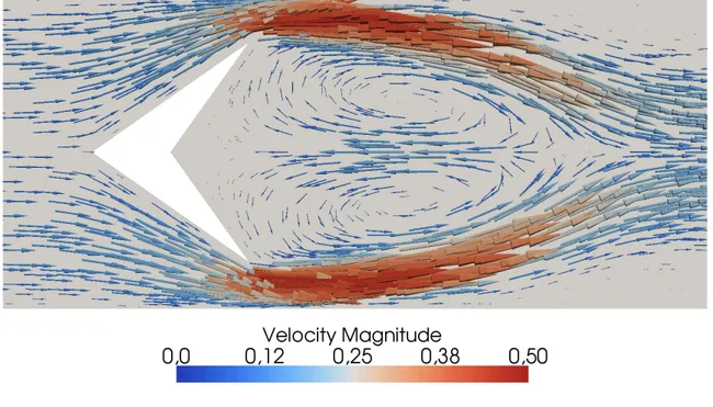
Figure 1.6.: Incompressible viscous flow in a channel with obstacle (image provided by Felix Heimann).
where shear viscosityµis a parameter of the fluid and therate of strain tensor D(v) = 1
2
�∇v+ (∇v)T�
. (1.34)
There are three new terms in the Navier-Stokes equations (1.32) compared to the Euler equa- tions (1.25). The last term on the right hand side of the momentum equation describes the forces due to internal friction. The termτ(v)vin the energy equation describes the energy flux due to internal friction and−λ∇T describes the heat conduction (TemperatureT is a function of the state variables). Depending on the application, e.g. in star formation, heat transfer might also include the effect of radiation.
A full derivation of the new terms in the Navier-Stokes equations is beyond the scope of these lecture notes, we refer e.g. to [Chung, 1996] for details. Note however, that all the new terms involve second derivatives, i.e. the Navier-Stokes equations are a second-order system of PDEs.
Incompressible Viscous Flow
In many applications the fluid can be regarded as incompressible which means that density is independent of pressure. If temperature variations are also insignificant it is a constant.
Neglecting also the energy equation (because temperature is assumed to have no effect on the fluid) and assuming that the fluid enters and leaves the domain only via the boundary (m=0)
u(n)0 u(n)1 m1
m2 u(n)2
u(n)n
mn
u(n)n+1
f(n)1
f(n)2
f(n)n
x z
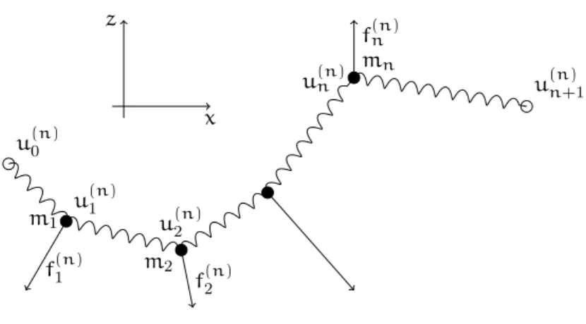
Figure 1.7.: Discrete mass-spring system.
results in the system of equations known as the incompressible Navier-Stokes equations:
∇ ·v=0, (1.35a)
∂tv+∇ ·(vvT) −ν∆v+∇p=f, (1.35b) with the kinematic viscosity ν = µ/ρ. Here p (which has been rescaled by 1/ρ) is now an independent variable to be determined. In order to derive the momentum equation (1.35b) the incompressibility constraint∇ ·v=0 has been applied twice: once to simplify the stress tensor τ and a second time to conclude∇ ·D(u) =∆u.
Figure 1.6 shows an example of incompressible, laminar flow around an obstacle in a two- dimensional channel.
1.3. Calculus of Variations
In this section we present a general approach that is used to study many mechanical and geo- metrical problems. For simplicity it will be illustrated by modelling the deflection of an elastic string where it leads to a two-point boundary value problem in ordinary differential equations.
The general principle, however, applies to the multi-dimensional situation and is essential to understand the finite element method for the numerical solution of partial differential equations.
1.3.1. Equilibrium Principle
We are interested in modelling the deflection of an elastic string under a load. As an example consider a string where cloth is put on for drying. The property of elasticity means that after the load is removed the string returns exactly to its unloaded position without any lasting effect. In order to derive the model we will first consider systems of finitely many straight and ideal springs connected together. Then we will to a continuum by an appropriate limit process.
Discrete Spring System
Figure 1.7 shows the system of n ∈ N point masses m1, . . . ,mn located at the positions u(n)0 , . . . ,u(n)n and connected by springs. Assuming all forces are applied in a plane we have
u(n)i ∈R2. Springi, 0�i�n, is elongated from positionu(n)i to position u(n)i+1 with the two endpoints
u(n)0 =
� xa
za
�
, u(n)n+1=
� xb
zb
�
(1.36) held fixed. All interior positions to be determined are collected in a big vector
u(n)= (u(n)1 , . . . ,u(n)n )T ∈R2n
which completely describes the state of the system. At each positionu(n)i , 1�i�n, a force given by the vectorf(n)i ∈R2 is applied.
In order to place the system in the stateu(n)work has to be done against the forces excerted by the springs and the forcesfi. This work is stored as elastic energyJ(n)el and potential energy J(n)f (in physics elastic energy is also a form of potential energy but for ease of writing we stick to these names). We now consider both energies separately.
The magnitude of the force excerted by a single spring extended to length l is given by Hooke’s law
F(l) =κ(l−l0)
whereκis the spring constant with units N m−1andl0the length of the unloaded spring. The work done when extending the spring from lengthl0 tolis then
Wel(l) =
�l
l0
F(s)ds=
�l
l0
κ(s−l0)ds=�κ
2(s−l0)2�l l0 = κ
2(l−l0)2. Then the total elastic energy in all springs in stateu(n)is
J(n)el (u(n)) = 1 2
�n i=0
κi(�u(n)i+1−u(n)i �−li)2 (1.37) whereκi andli are the individual spring parameters.
The work done to bring a mass m to positionuagainst the exterior force fis given by the path integral
Wf(u) = −
�u
0 f·t ds= −�u−0� u−0
�u−0�·f= −f·u.
Here we used 0 as the reference point but any other position is also in order. Note that when u·fis negative (e.g. the mass is lifted up in the gravity field f= (0,−mg)T pointing down) then the potential energy increases. The potential energy of all mass points is then
J(n)f (u(n)) = −
�n i=1
f(n)i ·u(n)i (1.38)
and the total (potential) energy stored in the system at stateu(n) is J(n)(u(n)) =J(n)el (u(n)) +J(n)f (u(n)) = 1
2
�n i=0
κi(�u(n)i+1−u(n)i �−li)2−
�n i=1
f(n)i ·u(n)i . (1.39)
The equilibrium principle in mechanics says that the stateu(n)∗ attained by the system at equilibrium is the state of minimal (potential) energy:
J(n)(u(n)∗ )�J(n)(u) ∀u∈R2n. A short notation of the same statement is
u(n)∗ = argmin
u∈R2n J(n)(u). (1.40)
Note that problem (1.40) does in general not have a unique solution. An example for nonuniquess is the case f(n)i = 0 for all i and �n
i=0li > �u(n)n+1 −u(n)0 � where infinitely many solutions exist. When the endpoints of the string are sufficently far apart, however, one can prove that the functional J(n)(u)can be bounded from below, i.e.
J(n)(u)�C ∀u∈R2n (1.41)
and that it is convex, i.e.
J(n)(θu+ (1−θ)v)�θJ(n)(u) + (1−θ)J(n)(v) ∀u,v∈R2n,θ∈[0, 1]. (1.42) By analogy with functions in one variable we may conclude that the problem has a unique global minimum. We will prove such a result later in a related context.
Continuum Limit
We now aim at describing the position of the string by a continuous curveu:I= [0, 1]→R2. The parameter interval I is in principle arbitrary and the equations to be derived should not depend on the particular parametrization. A number ξ ∈ I is used to “label” a point on the string and is called material coordinate. The space R2 of positions is called the configuration space in this context.
To go from the discrete to the continuum model we introduce for everyn∈Na discretization of the parameter interval
ξ(n)i = i n+1
with the idea that u(ξ(n)i )corresponds to positionu(n)i of the discrete spring model. Further- more we assume that the total length of the unloaded and unclamped string is given by Land set the lengths of the individual strings to
l(n)i = L n+1.
With the abbreviationξ(n)i±1/2= 12(ξ(n)i +ξ(n)i±1)the other parameters of the discrete system are
κ(n)i =κ(ξ(n)i+1/2), f(n)i =
�ξ(n)i+1/2
ξ(n)i−1/2
f(ξ)dξ
where κ : I→ R is a given continuous function describing the elastic properties of the string and f: I →R2 is an integrable function giving the load density with units N m−1. Inserting
these definitions into Equation (1.37) for the discrete elastic energy yields (with slight abuse of notation):
J(n)el (u) = 1 2
�n i=0
κi(�u(ξ(n)i+1) −u(ξ(n)i �−li)2
= 1 2
�n i=0
κi
��u(ξ(n)i+1) −u(ξ(n)i �
ξ(n)i+1−ξ(n)i (ξ(n)i+1−ξ(n)i ) − L n+1
�2
= 1 2
�n i=0
κi(ξ(n)i+1−ξ(n)i )2
����
��
u(ξ(n)i+1) −u(ξ(n)i ξ(n)i+1−ξ(n)i
��
��
�−L
�2
(1.43)
where we usedξ(n)i+1−ξ(n)i =1/(n+1). At this point we need to reconsider the spring “constant”
κ. It has units N m−1and depends on the length of the spring. This becomes important as the length of the individual springs now decreases asn increases. Mechanics tells us that a spring with cross-sectional areaAi, modulus of elasticityEi and lengthli has a spring “constant”
κi= AiEi
li = AiEi
L/(n+1) = ˜κ(ξ(n)i+1/2) L(ξ(n)i+1−ξ(n)i ).
Note that the new material property function ˜κ(ξ) has units N and is now independent of the length of the string. Inserting this expression into Equation (1.43) yields
J(n)el (u) = 1 2
�n i=0
˜ κi
L
����
��
u(ξ(n)i+1) −u(ξ(n)i ξ(n)i+1−ξ(n)i
��
��
�−L
�2
(ξ(n)i+1−ξ(n)i ) where we can now pass to the limit
Jel(u) = lim
n→∞J(n)el (u) =
�1 0
˜ κ(ξ)
2L
��u�(ξ)�−L�2
dξ. (1.44)
Hereby we assumed that the derivativeu�(ξ)is well defined, i.e.u∈�
C1([0, 1])�2 Now the potential energy is .
J(n)f (u) = −
�n i=1
f(n)i ·u(ξ(n)i ) = −
�n i=1
�ξ(n)i+1/2
ξ(n)i−1/2
f(ξ)·u(ξ(n)i ) and passing to the limit gives
Jf(u) = lim
n→∞J(n)f (u) = −
�1
0f(ξ)·u(ξ).
As in the discrete case we have J(u) =Jel(u) +Jf(u) =
�1
0
˜ κ(ξ)
2L
��u�(ξ)�−L�2
−f(ξ)·u(ξ)dξ. (1.45)
Application of the equilibrium principle now results in a minimization problem in function space
u∗= argmin
u∈V J(u) (1.46)
where the space of all admissible functionsV is V =
� v∈�
C1([0, 1])�2
: v(0) =
� xa za
�
,v(1) =
� xb zb
��
(1.47) since u�(ξ) turns up in the energy functional. This now raises the question how to solve a minimization problem in function space?
1.3.2. Variational Approach
To find the minimum of a functiong(x)in one real variable one searches for stationary points g�(x∗) =0 and then checks whetherx∗really is a minimum. Transfering this idea to minimiza- tion problems in function space such as (1.46) is the central idea of the calculus of variations.
As in the case of a function in one variable the search for stationary points of the functional J(u)results only in a necessary condition for a minimum.
To start let us rewrite the minimization property as:
u∗= argmin
u∈V J(u) ⇔ J(u∗)�J(u∗+tv) ∀t∈R,∀v∈V0 where
V0=
� v∈�
C1([0, 1])�2
: v(0) =v(1) =
� 0 0
��
. (1.48)
The function vis called avariation or test function and the definition of V0 ensures that the functionu∗+tvalways satisfies the given boundary conditions which are already incorporated in u∗. The energy functional J(u) to be minimized is called Lagrangian in the calculus of variations and the function spacesV andV0 are called trial space andtest space respectively.
Now the functionφ(t) =J(u∗+tv)is an ordinary function in one variable for a fixedv∈V0. If dφdt exists then we have
J(u∗)�J(u∗+tv) ∀t∈R,∀v∈V0 ⇒ dφ
dt(0) =0 ∀v∈V0. (1.49) The reverse conclusion can also be shown if the minimizer exists. Now let us compute the configurational derivative dφdt. For any givenu∈V, v∈V0 we get
d
dtJf(u+tv) = d dt
�
−
�1
0f(ξ)·(u(ξ) +tv(ξ))dξ
�
= −
�1
0f(ξ)·v(ξ)dξ and so
d
dtJf(u+tv)���
t=0= −
�1
0f(ξ)·v(ξ)dξ.
For the more complicated elastic part we get d
dtJel(u+tv) = d dt
�1
0
˜ κ(ξ)
2L
��u�(ξ) +tv�(ξ)�−L�2
=
�1
0
˜ κ(ξ)
L
��u�(ξ) +tv�(ξ)�−L�[u�(ξ) +tv�(ξ)]·v�(ξ)
�u�(ξ) +tv�(ξ)� dξ
where we have used dtd�x+ty�= (x+ty)·y/�x+ty�for any two vectorsx,y∈Rn and the Euclidean scalar product and norm. By settingt=0 we get
d
dtJel(u+tv)
��
�t=0=
�1
0
˜ κ(ξ)
L
�u�(ξ)�−L
�u�(ξ)� u�(ξ)·v�(ξ)dξ.
Putting both parts together results in the necessary condition foru (we refrain from writing u∗ for the minimum from now on!) being a minimizer of the functionalJ(u):
�1
0
˜ κ(ξ)
L
�u�(ξ)�−L
�u�(ξ)� u�(ξ)·v�(ξ) −f(ξ)·v(ξ)dξ=0 ∀v∈V0. (1.50) This equation is called a (nonlinear)variational equation.
Abstract Variational Problem For a general Lagrangian of the form
J(u) =
�1
0F(u�(ξ),u(ξ))dξ we get by applying the chain rule the variational equation
d
dtJ(u+tv)
��
�t=0= d dt
��1
0 F(u�(ξ) +tv�(ξ),u(ξ) +tv(ξ))dξ
�����
�t=0
=
�1
0∂1F(u�(ξ),u(ξ))v�(ξ) +∂2F(u�(ξ),u(ξ))v(ξ)dξ=0 ∀v∈V0
(1.51)
where ∂1F, ∂2F denote the partial derivatives of F with respect to the first and second argu- ment. Note that the variationvalways enterslinearly in this equation! Therefore, the general variational equation has the abstract form:
Findu∈V : r(u,v) =0 ∀v∈V0 (1.52) wherer:V×V0→Ris linear in v, i.e.
r(u,v1+v2) =r(u,v1) +r(u,v2), r(u,kv) =kr(u,v)
but possibly nonlinear in u. In the applications the test space V0 is a real vector space of functions and V is an affine space V = u0+V0 ={u : u=u0+v,v∈V0} incorporating the boundary conditions.
A note on the requirement of the differentiability of u andv. The minimization problem as well as the variational problem were derived under the assumption that u,v ∈ �
C1([0, 1])�2
It will turn out that this function space is neither appropriate for proving the existence of a. solution nor practical for the applications (consider for example a pointwise load on the string).
Differential Equation
Integrating by parts the first term in Equation (1.51) gives
�1
0∂1F(u�(ξ),u(ξ))v�(ξ) +∂2F(u�(ξ),u(ξ))v(ξ)dξ
=
�1
0− d dξ
�∂1F(u�(ξ),u(ξ))�
v(ξ) +∂2F(u�(ξ),u(ξ))v(ξ)dξ +�
∂1F(u�(ξ),u(ξ))v(ξ)�1 0
where the boundary term vanishes due to the boundary condition on v! In order to do the integration by parts it is necessary to assume thatFis now twice differentiable with respect to each variable and also that u∈ �
C2([0, 1])�2
. This leads then to the following variant of the variational equation
�1
0
�
− d
dξ∂1F(u�(ξ),u(ξ)) +∂2F(u�(ξ),u(ξ))
�
v(ξ)dξ=0 ∀v∈V0.
Now the fundamental lemma of the calculus of variation states that if this equation is true for all test functions vthen the function in square brackets must vanish pointwise:
− d
dξ∂1F(u�(ξ),u(ξ)) +∂2F(u�(ξ),u(ξ)) =0 (ξin(0, 1)). (1.53) Equation (1.53) is a nonlinear two-point boundary value problem called the Euler-Lagrange equation for the variational problem (1.51). Note the similarity to the reasoning in §1.2.2 when going from Equation (1.10) to (1.11). There we applied Gauss’ theorem to the arbitrary domain ω ⊆ Ω which can be interpreted as a special case of integration by parts with a piecewise constant function (the characteristic function of ω).
Setting up the Euler-Lagrange equation for our string example, i.e. applying integration by parts to Equation (1.50), results in the nonlinear second-order ordinary differential equation
− d dξ
�˜κ(ξ) L
�u�(ξ)�−L
�u�(ξ)� u�(ξ)
�
=f(ξ) (ξin(0, 1)) with boundary values
u(0) =
� xa
za
�
, u(1) =
� xb zb
� .
Note that for this equation to make sense for us at the moment we require ˜κ∈C1([0, 1]) and u∈�
C2([0, 1])�2
In summary, we now have the following situation.
⇒ ⇒
Minimization problem(I)
u= argmin
v∈V J(v)
Variational problem(II) Findu∈V such that
r(u,v) =0 ∀v∈V0
(III)
Differential equation Solve BVB g(u,u�,u��) =0 inΩ
ugiven on∂Ω
For step (I)→(II) we introduced the concept of the configurational derivative. We will later see that (I) follows also from (II) provided that the minimum exists. For the step (II)→(III) we applied integration by parts and had to assume additional smoothness for the solution and coefficient functions. In general, a solution of problem (II) need not be a solution of problem (III) therefore. By taking the perspective of the differential equation the variational problem (II) is called theweak formulation of the boundary value problem.
1.3.3. Taut String Approximation
In this paragraph we are interested in the situation where the length Lof the string with zero elastic energy is much shorter than the distance of the two points where it is clamped to, i.e.
L� �u(1) −u(0)�.
Under this assumption we get
L� �u(1) −u(0)�=
��
��
�1
0u�(ξ)dξ
��
����1
0�u�(ξ)�dξ. With this the energy functional (1.45) simplifies to
J(u) =
�1
0
˜ κ(ξ)
2L
��u�(ξ)�−L�2
−f(ξ)·u(ξ)dξ
≈
�1 0
˜ κ(ξ)
2L �u�(ξ)�2−f(ξ)·u(ξ)dξ=:˜J(u).
Now ˜J(u)is aquadratic functional inu. The associated variational problem is u∈V :
�1
0
˜ κ(ξ)
2L u�(ξ)v�(ξ) −f(ξ)·v(ξ)dξ=0 ∀v∈V0 (1.54) which is now a linear variational problem in u. The related differential equation is then also linear and reads
− d dξ
�κ(ξ)˜ L
du dξ
�
=f in(0, 1) (1.55)
which decouples into two seperate equations forx(ξ)and z(ξ).
Let us assume now the special situation where there is only a vertical loadf(ξ) = (0,fz(ξ))T. Naming the componentsu(ξ) = (x(ξ),z(ξ))T andv(ξ) = (φ(ξ),ψ(ξ))T the variational problem (1.54) reads
u∈V :
�1
0
˜ κ(ξ)
2L (x�(ξ)φ�(ξ) +z�(ξ)ψ�(ξ)) −fz(ξ)ψ(ξ)dξ
=
�1 0
˜ κ(ξ)
2L x�(ξ)φ�(ξ)dξ+
�1 0
˜ κ(ξ)
2L z�(ξ)ψ�(ξ)) −fz(ξ)ψ(ξ)dξ=0 ∀φ,ψ∈C10([0, 1]).
The equation forx(ξ)can be solved analytically by solving the corresponding differential equa- tion and we find:
x(ξ) =xa+ (xb−xa)
�ξ
0 L
˜ κ(s)ds
�1 0 L
˜ κ(s)ds.
Since Land ˜κ are strictly positive quantities the function ξ→ x(ξ) is strictly increasing and therefore has an inverse x→x−1(x).
We now want to write the second componentz(ξ)as a function ofx(ξ)instead ofξ. Therefore we define the new function ˆz(x) and use the chain rule:
z(ξ) =ˆz(x(ξ)) ⇒ dz
dξ(ξ) = dˆz
dx(x(ξ))dx dξ(ξ).
The same applies for the test function ψ(x) =ψ(x(ξ)). Recalling the transformation theoremˆ for integrals �b
ag(s)ds = �b�
a�g(µ(t))|dµdt(t)|dt with µ: [a�,b�] → [a,b] a differentiable map, we obtain for the variational problem for the second component z(ξ):
�1 0
˜ κ(ξ)
2L ˆ z
dx(x(ξ))dx dξ(ξ)ψˆ
dx(x(ξ))dx
dξ(ξ) −fz(ξ)ψ(x(ξ))ˆ dξ
=
�xb
xa
�κ(x˜ −1(x)) 2L
dˆz dx(x)
�dx
dξ(x−1(x))
�2dψˆ
dx(x) −fz(x−1(x))ψ(x)ˆ
�� 1
��dξdx(x−1(x))
��
� dx
=
�xb
xa
˜
κ(x−1(x)) 2L
��
��dx
dξ(x−1(x))
��
��
� �� �
ˆ σ(x)
dˆz dx(x)dψˆ
dx(x) − fz(x−1(x))
��
�dxdξ(x−1(x))
��
� �� ��
f(x)ˆ
ψ(x)ˆ dx=0 ∀ψ∈C10([xa,xb]).
The corresponding linear second-order scalar differential equation for the function ˆz now in
“physical coordinates” reads:
− d dx
� ˆ σ(x)dˆz
dx
�
=f(x)ˆ in(xa,xb) with boundary conditions
ˆ
z(xa) =za, ˆz(xb) =zb. In two space dimensions the equation
−∇ ·(σ(x)∇u) =f inΩ⊂R2 with boundary conditions
u=g on ∂Ω (1.56)
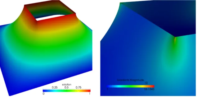
is a model for the vertical position of a thin sheet of rubber under vertical load that is clamped at the boundary. Figure 1.8 shows an example for the two-dimensional case. Note that �∇u� can become very large near so-called “reentrant corners” of the domain.
1.3.4. Linear Elasticity and Plate Problem
The considerations of this Section can be generalized to a small deformations of a three- dimensional elastic material experiencing both tension and compression. The resulting energy functional for thelinear elasticity problem is
J(u) =
�
Ω
1 2
�λ(∇ ·u)2+2µD(u) :D(u)�
−f·u dx (1.57)