Numerical Methods for Partial Diﬀerential Equations

(1)

Numerical Methods for Partial Differential Equations

Steffen B¨ orm

Compiled August 19, 2020, 16:33

(2)

(3)

1. Introduction

Differential equations have been established as one of the most important representations of the laws governing natural phenomena, e.g., the movement of bodies in a gravitational field or the growth of populations.

If all functions appearing in the equation depend only on one variable, we speak of anordinary differential equation. Ordinary differential equations frequently describe the behaviour of a system over time, e.g., the movement of an object depends on its velocity, and the velocity depends on the acceleration.

Ordinary differential equations can be treated by a variety of numerical methods, most prominently by time-stepping schemes that evaluate the derivatives in suitably chosen points to approximate the solution.

If the functions in the equation depend on more than one variable and if the equation therefore depends on partial derivatives, we speak of apartial differential equation. Par- tial differential equations can be significantly more challenging than ordinary differential equations, since we may not be able to split the computation into discrete (time-)steps and have to approximate the entire solution at once.

A typical example is thepotential equation of electrostatics. Given a domain Ω⊆R³, we consider

∂²u

∂x²₁(x) +∂²u

∂x²₂(x) +∂²u

∂x²₃(x) =f(x) for all x∈Ω, where ^∂_∂x^ν^uν

i denotes the ν-th partial derivative with respect to the i-th variable.

Explicit solutions for this equation are only known in special situations, e.g., if Ω =R³ or Ω = [a1, b1]×[a2, b2]×[a3, b3], while the general case usually has to be handled by numerical methods.

Since computers have only a finite amount of storage at their disposal, they are generally unable to represent the solution u as an element of the infinite-dimensional space C²(Ω) exactly. Instead we look for an approximation of the solution in a finite- dimensional space that can be represented by a computer. Since the approximation is usually constructed by replacing the domain Ω by a grid of discrete points, the approximation of the solution is called adiscretization.

A fairly simple discretization technique is the method offinite differences: we replace the derivatives by difference quotients and replace Ω by a grid Ωhsuch that the difference quotients in the grid points can be evaluated using only values in grid points. In the case of the potential equation, this leads to a system of linear equations that can be solved in order to obtain an approximation uh ofu.

We have to investigate thediscretization error, i.e., the difference betweenu_h anduin the grid points. This task can be solved rather elegantly by establishing theconsistency

(6)

and the stability of the discretization scheme: consistency means that applying the approximated derivatives to the real solution u yields an error that can be controlled, and stability means that small perturbations of the forcing term f lead only to small perturbations of the solution u_h. Once both properties have been established, we find that the discretization scheme isconvergent, i.e., that we can reach any given accuracy as long as we use a sufficiently fine grid.

For time-dependent problems like the heat equation and the wave equations, it is a good idea to treat the time variable separately. An attractive approach is the method of lines that uses a discretization in space to obtain a system of ordinary differential equations that can be treated by standard time-stepping algorithms.

Since the Lipschitz constant arising in this context is quite large, it is a good idea to consider implicit time-stepping schemes that provide better stability and do not require us to use very small time steps in order to avoid oscillations.

The wave equation conserves the total energy of the system, and we would like to have a numerical scheme that shares this property. If we replace the total energy by a suitable discretized counterpart, we find that theCrank-Nicolson method guarantees that the discretized total energy indeed remains constant.

In order to prove consistency of finite difference methods, we frequently have to assume that the solutionuis quite smooth, e.g., a standard approach for the potential equation requiresuto be four times continuously differentiable. This is an assumption that is only rarely satisfied in practice, so we have to consider alternative discretization schemes.

Variational methods are particularly attractive, since they are based on an elegant reformulation of the partial differential equation in terms of Hilbert spaces. We can prove that the variational equation has a unique generalized solution in aSobolev space, and that this generalized solution coincides with the classical solution if the latter exists.

Variational formulations immediately give rise to theGalerkin discretizationscheme that leads to a system of equations we can solve to obtain an approximation of the solution.

If we use a finite element method, this system has a number of desirable properties, most importantly it is sparse, i.e., each row of the corresponding matrix contains only a small number of non-zero entries. This allows us to apply particularly efficient solvers to obtain the approximate solution.

In order to be able to approximate the solution even with fairly weak regularity as- sumptions, we investigate the approximation properties of averaged Taylor polynomials and obtain theBramble-Hilbert lemma, a generalized error estimate for these polynomials, and the Sobolev lemma, an embedding result for Sobolev spaces that allows us to use standard interpolation operators to construct the finite element approximation.

Acknowledgements

I would like to thank Jens Liebenau, Alexander Dobrick, Mario Santer, Nils Kr¨utgen, and Jonas Lorenzen for corrections and suggestions for improvements of these lecture notes.

(7)

2. Finite difference methods

This chapter provides an introduction to a first simple discretization technique for elliptic partial differential equations: the finite difference approach replaces the domain by a grid consisting of discrete points and the derivatives in the grid points by difference quotients using only adjacent grid points. The resulting system of linear equations can be solved in order to obtain approximations of the solution in the grid points.

2.1. Potential equation

A typical example for anellipticpartial differential equation is thepotential equation, also known as Poisson’s equation. As its name suggests, the potential equation can be used to find potential functions of vector fields, e.g., the electrostatic potential corresponding to a distribution of electrical charges.

In the unit square Ω := (0,1)×(0,1) the equation takes the form

−∂²u

∂x²₁(x)−∂²u

∂x²₂(x) =f(x) for all x= (x1, x2)∈Ω.

In order to obtain a unique solution, we have to prescribe suitable conditions on the boundary

∂Ω := Ω∩R²\Ω ={0,1} ×[0,1]∪[0,1]× {0,1}

of the domain. Particularly convenient for our purposes areDirichlet boundary conditions given by

u(x) = 0 for all x= (x₁, x₂)∈∂Ω.

In the context of electrostatic fields, these conditions correspond to a superconducting boundary: if charges can move freely along the boundary, no potential differences can occur.

In order to shorten the notation, we introduce theLaplace operator

∆u(x) = ∂²u

∂x²₁(x) +∂²u

∂x²₂(x) for all x= (x₁, x₂)∈Ω, and summarize our task as follows:

Find u∈C( ¯Ω) with u|_Ω ∈C²(Ω), and

−∆u(x) =f(x) for allx∈Ω, (2.1a)

u(x) = 0 for allx∈∂Ω. (2.1b)

(8)

Solving this equation “by hand” is only possible in special cases, the general case is typically handled by numerical methods.

The solutionuis an element of an infinite-dimensional space of functions on the domain Ω, and we can certainly not expect a computer with only a finite amount of storage to represent it accurately. That is why we employ adiscretization, in this case of the domain Ω: we replace it by a finite number of discrete points and focus on approximating the solution only in these points.

Using only discrete points means that we have to replace the partial derivatives in the equation by approximations that require only the values of the function in these points.

Lemma 2.1 (Central difference quotient) Leth∈R>0 andg∈C⁴[−h, h]. We can findη∈(−h, h) with

g(h)−2g(0) +g(−h)

h² =g⁰⁰(0) + h²

12g⁽⁴⁾(η).

Proof. Using Taylor’s theorem, we findη+∈(0, h) and η−∈(−h,0) with g(h) =g(0) +hg⁰(0) + h²

2 g⁰⁰(0) + h³

6 g⁰⁰⁰(0) + h⁴

24g⁽⁴⁾(η₊), g(−h) =g(0)−hg⁰(0) + h²

2 g⁰⁰(0)−h³

6 g⁰⁰⁰(0) + h⁴

24g⁽⁴⁾(η−).

Adding both equations yields

g(h) +g(−h) = 2g(0) +h²g⁰⁰(0) +h⁴ 12

g⁽⁴⁾(η₊) +g⁽⁴⁾(η−)

2 .

Since the fourth derivativeg⁽⁴⁾ is continuous, we can apply the intermediate value theorem to findη ∈[η−, η+] with

g⁽⁴⁾(η) = g⁽⁴⁾(η+) +g⁽⁴⁾(η−) 2

and obtain

g(h)−2g(0) +g(−h) =h²g⁰⁰(0) +h⁴

12g⁽⁴⁾(η).

Dividing byh² gives us the required equation.

Exercise 2.2 (First derivative) Let h∈R>0 andg∈C²[0, h]. Prove that there is an η∈(0, h) such that

g(h)−g(0)

h =g⁰(0) + h 2g⁰⁰(η).

Let nowg∈C³[−h, h]. Prove that there is an η∈(−h, h) such that g(h)−g(−h)

2h =g⁰(0) +h² 6 g⁰⁰⁰(η).

(9)

2.1. Potential equation Applying Lemma 2.1 to the partial derivatives with respect tox₁ and x₂, we obtain the approximations

2u(x₁, x₂)−u(x₁+h, x₂)−u(x₁−h, x₂)

h² = ∂²u

∂x²₁(x) +h² 12

∂⁴u

∂x⁴₁(η₁, x₂), (2.2a) 2u(x₁, x₂)−u(x₁, x₂+h)−u(x₁, x₂−h)

h² = ∂²u

∂x²₂(x) +h² 12

∂⁴u

∂x⁴₂(x₁, η₂), (2.2b) with suitable intermediate points η1∈[x1−h, x2+h] undη2 ∈[x2−h, x2+h]. Adding both equations and dropping theh² terms leads to the approximation

∆_hu(x) = u(x₁+h, x₂) +u(x₁−h, x₂) +u(x₁, x₂+h) +u(x₁, x₂−h)−4u(x₁, x₂) h²

(2.3) f¨ur alle x∈Ω, h∈H_x

of the Laplace operator, where the set

Hx:={h∈R>0 : x1+h∈[0,1], x1−h∈[0,1], x2+h∈[0,1], x2−h∈[0,1]}

describes those step sizes for which the difference quotient can be evaluated without leaving the domain Ω. The approximation (2.3) is frequently called a five point star, since the values of u are required in five points in a star-shaped pattern centered atx.

In order to quantify the approximation error, we introduce suitable norms on function spaces.

Reminder 2.3 (Maximum norm) For real-valued continuous functions on a compact set K, we define the maximum norm by

kuk∞,K := max{|u(x)| : x∈K} for all u∈C(K).

For vectors with a general finite index set I, we let

kuk_∞:= max{|u_i| : i∈ I} for all u∈R^I. Lemma 2.4 (Consistency) If u∈C⁴( ¯Ω) holds, we have

|∆_hu(x)−∆u(x)| ≤ h²

6 |u|_4,Ω for allx∈Ω, h∈Hx, (2.4) where we use the semi-norm

|u|_4,Ω := max (

∂^ν+µu

∂x^ν₁∂x^µ₂ ∞,Ω¯

: ν, µ∈N0, ν+µ= 4 )

on the right-hand side that is defined by the maximum norm of the fourth derivatives.

(10)

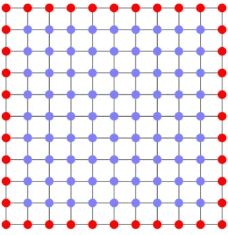
Figure 2.1.: Grid for N = 9

Proof. We add the equations (2.2) and bound the fourth derivatives by |u|_4,Ω.

Compared to the differential operator ∆, thedifference operator ∆_h offers the advantage that only values of the function in a small number of discrete points are required.

We can use this property to replace the domain Ω by a finite set of points that is far better suited for computers.

Definition 2.5 (Grid) Let N ∈N, and let h:= 1

N + 1,

Ω_h :={(ih, jh) : i, j∈ {1, . . . , N}} ⊆Ω,

∂Ω_h :={(ih,0),(ih,1),(0, jh),(1, jh) : i, j∈ {0, . . . , N+ 1}} ⊆∂Ω, Ω¯_h := Ω_h∪∂Ω_h.

We callΩ_h, ∂Ω_h andΩ¯_h grids for the setsΩ, ∂Ω and Ω.¯ Restricting the estimate (2.4) to the grid Ωh yields

| −∆hu(x)−f(x)|=| −∆hu(x) + ∆u(x)| ≤ h²

6 kuk_4,Ω¯ for all x∈Ω, and this property suggests that we look for a solution of the equation−∆_hu=f, since we may hope that it will approximate the “real” solutionu. Since the evaluation of ∆hu in x ∈ Ω_h requires only values in points of ¯Ω_h, we introduce functions that are only defined in these points.

(11)

2.2. Stability and convergence

Definition 2.6 (Grid function) Let Ω_h and Ω¯_h grids forΩ and Ω. The spaces¯ G(Ω_h) :={u_h : u_h mapsΩ_h to R},

G( ¯Ωh) :={u_h : uh mapsΩ¯h to R}

are called spaces of grid functions from Ω_h and Ω¯_h, respectively, to R. The space G0( ¯Ωh) :={u_h∈G( ¯Ωh) : uh(x) = 0 for allx∈∂Ωh}

is called the space of grid functions with homogeneous Dirichlet boundary conditions.

The difference operator ∆_h is obviously a linear mapping from G( ¯Ω_h) toG(Ω_h), and we can approximate the differential equation (2.1) by the following system of linear equations:

Find a grid functionuh∈G0( ¯Ωh) such that

−∆_hu_h(x) =f(x) for all x∈Ω_h. (2.5) Since this system of linear equations (each pointx∈Ωh corresponds to a linear equation thatu_hhas to satisfy) is defined on the set Ω_hof discrete points instead of the continuous set Ω, we call (2.5) adiscretizationof the potential equation (2.1). In this particular case, all differential operators are replaced by difference quotients involving a finite number of values, giving this approach the name finite difference method.

2.2. Stability and convergence

Merely formulating the discrete system (2.5), is not enough, we also have to investigate whether this system can be solved, whether the solution is unique, and whether it approximates the continuous solutionu.

If is easy to see that−∆_h is a linear mapping from G₀( ¯Ω_h) to G(Ω_h) and that dimG0( ¯Ω_h) = dimG(Ω_h) =N²

holds. In order to prove that the system (2.5) has a unique solution, it is enough to prove that −∆_h is an injective mapping.

A particularly elegant way of proving this result is to use the following stability result for the maximum norm:

Lemma 2.7 (Maximum principle) Letv_h ∈G( ¯Ω_h) denote a grid function satisfying

−∆_hv_h(x)≤0 for all x∈Ω_h. There exists a boundary point x₀∈∂Ω_h such that

v_h(x)≤v_h(x0) for all x∈Ω¯_h, i.e., the grid function takes its maximum at the boundary.

(12)

Proof. We define the sets of neighbours of pointsx by

N(x) :={(x₁−h, x₂),(x₁+h, x₂),(x₁, x₂−h),(x₁, x₂+h)} for all x∈Ω_h. The distance (with respect to the grid) from a grid point to the boundary is denoted by

δ: ¯Ω_h →N0, x7→

(0 ifx∈∂Ω_h, 1 + min{δ(x⁰) : x⁰ ∈N(x)} otherwise.

We denote the maximum ofv_h by

m:= max{v_h(x) : x∈Ω¯_h} and intend to prove by induction

(v_h(x) =m∧δ(x)≤d) =⇒ ∃x₀ ∈∂Ω_h: v_h(x₀) =m (2.6) for all d∈N0 and all x ∈Ω¯_h. This implication yields our claim since δ(x) is finite for allx∈Ω.¯

The base case d = 0 of the induction is straightforward: if x ∈ Ω¯_h with v_h(x) = m and δ(x) =d= 0 exists, the definition of δ already implies x ∈∂Ω_h, so we can choose x0 =x.

Let now d∈N0 satisfy (2.6). Let x∈Ω¯_h be given withδ(x) =d+ 1 andv_h(x) =m.

This impliesx∈Ω_h and we obtain X

x⁰∈N(x)

h⁻²(v_h(x)−v_h(x⁰)) = 4h⁻²v_h(x)− X

x⁰∈N(x)

h⁻²v_h(x⁰) =−∆_hv_h(x)≤0.

Since m =vh(x) is the maximum of vh, none of the summands on the left side of this inequality can be negative. Since the sum cannot be positive, all summands have to be equal to zero, and this implies

m=v_h(x) =v_h(x⁰) for all x⁰ ∈N(x).

Due toδ(x) =d+ 1, there has to be ax⁰∈N(x) withδ(x⁰) =d, and since we have just provenvh(x⁰) =m, we can apply the induction assumption to complete the proof.

The maximum principle already guarantees the injectivity of the differen operator

−∆_h and the existence of a unique solution.

Corollary 2.8 (Unique solution) The system of linear equations (2.5) has a unique solution.

Proof. Letu_h,u˜_h ∈G₀( ¯Ω_h) be given with

−∆_hu_h(x) =f(x) for all x∈Ω_h,

−∆_hu˜_h(x) =f(x) for all x∈Ω_h.

(13)

We let v_h :=u_h−u˜_h and obtain

∆hvh(x) = ∆huh(x)−∆hu˜h(x) =−f(x) +f(x) = 0 for all x∈Ωh. The requirements of Lemma 2.7 are fulfilled, so the grid function v_h has to take its maximum at the boundary∂Ω_h. Due tov_h∈G₀( ¯Ω_h), we havev_h|_∂Ω_h= 0, and therefore

v_h(x)≤0 for all x∈Ω_h.

We can apply the same argument to the grid function ˜vh:= ˜uh−uh =−v_h to obtain v_h(x) =−˜v_h(x)≥0 for all x∈Ω_h,

and this yields v_h = 0 andu_h= ˜u_h. We have proven that ∆_h is injective.

Due to dimG(Ωh) = dimG0( ¯Ωh), the rank-nullity theorem implies that ∆h also has to be surjective.

Since Lemma 2.7 only requires ∆_hv_h not to be negative in any point x ∈Ω_h, we can also use it to obtain the following stability result that guarantees that small perturbations of the right-hand side of (2.5) are not significantly amplified.

Lemma 2.9 (Stability) Let uh ∈G0( ¯Ωh) a grid function with homogeneous Dirichlet boundary conditions. We have

ku_hk_∞,Ω_h≤ 1

8k∆_hu_hk_∞,Ω_h.

Proof. (cf. [7, Theorem 4.4.1]) The key idea of our proof is to consider the function w: ¯Ω→R≥0, x7→ x1

2 (1−x1).

Since it is quadratic polynomial, we have |w|_4,Ω = 0, and we can combine

−∆w(x) = 1 for allx∈Ω with (2.4) to obtain

−∆_hw_h(x) = 1 for allx∈Ω_h with the grid function wh :=w|Ω¯h∈G( ¯Ωh).

We denote the minimum and maximum of−∆_hu_h by α:= min{−∆_hu_h(x) : x∈Ω_h}, β:= max{−∆_hu_h(x) : x∈Ω_h} and define

u⁺_h :=w_hβ.

(14)

This implies

−∆_hu⁺_h(x) =−∆_hw_h(x)β=β for allx∈Ω_h, so we also have

−∆_h(u_h−u⁺_h)(x) =−∆_hu_h(x)−β≤0 for allx∈Ω_h. Letx∈Ω_h. Lemma 2.7 yields a boundary point x₀ ∈∂Ω_h such that

u_h(x)−u⁺_h(x)≤u_h(x₀)−u⁺_h(x₀).

Due to the Dirichlet boundary conditions, we haveuh(x0) = 0 and conclude uh(x)≤u⁺_h(x)−u⁺_h(x0).

It is easy to prove 0≤w(z)≤1/8 for all z∈Ω¯h, which implies u⁺_h(x)−u⁺_h(x0)≤β/8.

Sincex is arbitrary, we have proven u_h(x)≤ 1

8β for all x∈Ω_h.

Since −u_h is bounded from above by −α, we can apply the same arguments to −u_h to get

u_h(x)≥ 1

8α for all x∈Ω_h.

Combining both estimates yields ku_hk_∞,Ω_h≤ 1

8max{|α|,|β|}= 1

8k∆_hu_hk_∞,Ω_h.

Combining this stability result with the consistency result of Lemma 2.4 we can prove theconvergence of our discretization scheme.

Theorem 2.10 (Convergence) Let u ∈ C⁴( ¯Ω) be the solution of (2.1, and let uh ∈ G₀(Ω_h) be the solution of (2.5). We have

ku−u_hk_∞,Ω_h ≤ h² 48|u|_4,Ω. Proof. Due to (2.1), we have

f(x) =−∆u(x) for allx∈Ω_h. The consistency result of Lemma 2.4 yields

|∆_hu(x)−∆_hu_h(x)|=|∆_hu(x) +f(x)|

(15)

=|∆_hu(x)−∆u(x)| ≤ h²

6 |u|_4,Ω for all x∈Ωh, which is equivalent to

k∆_h(u−uh)k_∞,Ω_h =k∆_hu−∆huhk_∞,Ω_h≤ h² 6 |u|_4,Ω. Now we can apply the stability result of Lemma 2.9 to get

ku−uhk∞,Ω_h ≤ 1

8k∆_hu−∆huhk∞,Ω_h≤ 1 8

h² 6 |u|_4,Ω.

If we can solve the linear system (2.5), we can expect the solution to converge to approximate u|_Ω_h at a rate of h². In order to express the linear system in terms of matrices and vectors instead of general linear operators, we have to introduce suitable bases for the spaces G₀( ¯Ω_h) and G(Ω_h). A straightforward choice is the basis (ϕ_y)y∈Ω_h

consisting of the functions ϕ_y(x) =

(1 ifx=y,

0 otherwise for all x∈Ω¯_h,

that are equal to one in y and equal to zero everywhere else and obviously form a basis of G₀( ¯Ω_h). Restricting the functions to G(Ω_h) yields a basis of this space, as well.

Expressing −∆_h in these bases yields a matrix L∈R^Ω^h^×Ω^h given by

(`_h)_x,y :=











4h⁻² ifx=y

−h⁻² if|x₁−y₁|=h, x₂ =y₂,

−h⁻² ifx₁=y₁, |x₂−y₂|=h,

0 otherwise

for allx, y∈Ω_h.

Expressing the grid function u_h and f_h in these bases yields vectors u_h,f_h ∈ R^Ω^h and the discretized potential equation (2.5) takes the form

L_hu_h=f_h. (2.7)

Since (2.5) has a unique solution, the same holds for (2.7).

The matrixL_h is particularly benign: a glance at the coefficients yields L_h =L^∗_h, so the matrix is symmetric. Applying the stability result of Lemma 2.9 to subsetsω_h⊆Ω_h shows that not only Lh is invertible, but also all of its principal submatrices Lh|_ω_h_×ω_h. This property guarantees that L_h possesses an invertible LR factorization that can be used to solve the system (2.7). We can even prove thatL_h is positive definite, so we can use the more efficient Cholesky factorization.

For large values ofN, i.e., for high accuracies, this approach is not particularly useful, since it does not take advantage of the special structure of L_h: every row and column

(16)

contains by definition not more than five non-zero coefficients. Matrices with the property that only a small number of entries per row or column are non-zero are calledsparse, and this property can be used to carry out matrix-vector multiplications efficiently and even to solve the linear system.

Exercise 2.11 (First derivative) If we approximate the one-dimensional differential equation

u⁰(x) =f(x) for all x∈(0,1)

by the central difference quotient introduced in Exercise 2.2, we obtain a matrix L ∈ R^N^×N given by

`_ij =







1/(2h) if j=i+ 1,

−1/(2h) if j=i−1,

0 otherwise,

for all i, j∈[1 :N].

Prove thatL is notinvertible if N is odd.

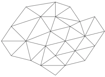
Remark 2.12 (General domains) Finite difference discretization are particularly well-suited for differential equations on “simple” domains like the unit square inves- tigated here. Treating more complicated domains requires us to use more involved techniques like the Shortley-Weller discretization and may significantly increase the complexity of the resulting algorithms.

2.3. Diagonal dominance and invertibility

The finite difference approach can be applied to treat more general partial differential equations: we simply have to replace all differential operators by suitable difference quotients. While the consistency of these schemes can usually be proven by using suitable Taylor expansions, the stability poses a challenge.

We investigate linear systems of equations

Ax=b (2.8)

with a matrixA ∈RÎ×I, a right-hand side b ∈RÎ and a solution x∈RÎ. A general- ization of the stability Lemma 2.9 would look like

kxk_∞≤CkAxk_∞ for allx∈R^I

with a constantC∈R≥0. This inequality can only hold if Ais injective, i.e., invertible, and we can rewrite it in the form

kA⁻¹bk∞≤Ckbk∞ for all b∈R^I by substitutingx=A⁻¹b.

(17)

2.3. Diagonal dominance and invertibility

We recall that any normk · kforR^I induces the operator norm kAk:= sup

kAxk

kxk : x∈R^I\ {0}

for all A∈R^I×I. (2.9) Stability therefore simply means that we have to be able to find an upper bound for kA⁻¹k_∞ that is independent of the mesh parameterh.

Lemma 2.13 (Neumann series) Let k · k be a norm for R^I, and let Let X∈R^I×I. If we have kXk<1, the matrix I−X is invertible with

∞

X

`=0

X^`= (I−X)⁻¹, k(I−X)⁻¹k ≤ 1 1− kXk. Proof. LetkXk<1. We define the partial sums

Ym:=

m

X

`=0

X^` for all m∈N0.

In order to prove that (Ym)^∞_m=0 is a Cauchy sequency, we first observe kY_m−Ynk=

m

X

`=n+1

X^`

≤

m

X

`=n+1

kXk^` =kXkⁿ⁺¹

m−n−1

X

`=0

kXk^`

≤ kXkⁿ⁺¹

∞

X

`=0

kXk^`= kXkⁿ⁺¹

1− kXk for all n, m∈N0 withn < m.

Given ∈R>0, we can find n0∈NwithkXkⁿ⁰⁺¹≤(1− kXk), and this implies kY_m−Y_nk ≤ kXkⁿ⁺¹

1− kXk ≤ kXkⁿ⁰⁺¹

1− kXk ≤ for all n, m∈N0, n₀≤n < m.

We conclude that (Ym)^∞_m=0 is a Cauchy sequency and therefore has a limit Y := lim

m→∞Y_m =

∞

X

`=0

X^`

satisfying

kYk=

∞

X

`=0

X^`

≤

∞

X

`=0

kXk^`= 1 1− kXk. Due to

(I−X)Y= (I−X)

∞

X

`=0

X^` =

∞

X

`=0

X^`−

∞

X

`=0

X^`+1 =

∞

X

`=0

X^`−

∞

X

`=1

X^` =I, Y(I−X) =

∞

X

`=0

X^`(I−X) =

∞

X

`=0

X^`−

∞

X

`=0

X^`+1 =

∞

X

`=0

X^`−

∞

X

`=1

X^` =I, we finally obtain Y= (I−X)⁻¹.

(18)

Exercise 2.14 (Generalized convergence criterion) Letk · kbe a norm forR^I and let X∈R^I×I. Assume that there is a k∈Nsuch that kX^kk<1. Prove

∞

X

`=0

X^` = (I−X)⁻¹, k(I−X)⁻¹k ≤ Pk−1

m=0kX^mk 1− kX^kk .

In order to be able to apply Lemma 2.13, we have to be able to find an upper bound for the operator norm. In the case of the maximum norm, this is particularly simple.

Lemma 2.15 (Maximum norm) We have kXk_∞= max

X

j∈I

|x_ij| : i∈ I

for all X∈R^I×I.

Proof. LetX∈R^I×I and set

µ:= max

X

j∈I

|x_ij| : i∈ I

.

Lety∈R^I and i∈ I. We have

|(Xy)_i|=

X

j∈I

xijyj

≤X

j∈I

|x_ij| |y_j| ≤X

j∈I

|x_ij| kyk∞≤µkyk∞

and concludekXk_∞≤µ.

Now we fixi∈ I such that

µ=X

j∈I

|x_ij|.

If we introduce the vectory∈R^I given by y_j :=

(−1 ifxij <0

1 otherwise for all j∈ I,

we findkyk_∞= 1 and µ=X

j∈I

|x_ij|=X

j∈I

xijyj = (Xy)i ≤ kXyk_∞= kXyk_∞

kyk ≤ kXk_∞.

Using the maximum norm and the Neumann series, we can find a simple criterion that allows us to check whether a given matrix is invertible: the diagonal elements have to be large enough.

(19)

2.3. Diagonal dominance and invertibility Definition 2.16 (Diagonally dominant matrices) A matrixA∈C^I×J withI ⊆ J is called weakly diagonally dominant if

X

j∈J j6=i

|a_ij| ≤ |a_ii| for all i∈ I.

It is called strictly diagonally dominant if X

j∈J j6=i

|a_ij|<|a_ii| for all i∈ I.

Using the Neumann series, it is possible to prove that strictly diagonally dominant matrices are invertible.

Lemma 2.17 (Strictly diagonally dominant) Let A ∈ C^I×I be strictly diagonally dominant. Then A is invertible.

Proof. SinceA is strictly diagonally dominant, we have

a_ii6= 0 for all i∈ I,

so the diagonal part D∈R^I×I of A, given by d_ij =

(aii ifi=j,

0 otherwise for alli, j ∈ I,

is invertible. The matrix

M:=I−D⁻¹A (2.10)

satisfies

mii= 1−aii

aii

= 0 for all i∈ I.

Since A is strictly diagonally dominant, we also have X

j∈I

|m_ij|=X

j∈I j6=i

|m_ij|=X

j∈I j6=i

|a_ij|

|a_ii| = 1

|a_ii| X

j∈I j6=i

|a_ij|<1 for all i∈ I,

and we can concludekMk_∞<1 by Lemma 2.15.

Now Lemma 2.13 yields that I−M=D⁻¹A is invertible, and this implies that the matrix Aitself also has to be invertible.

(20)

Remark 2.18 (Jacobi iteration) Lemma 2.17 is, in fact, not only a proof of the existence of the inverse A⁻¹, but also suggests a practical algorithm: in order to solve the linear system (2.8), we choose an arbitrary vector x⁽⁰⁾, and consider the sequence (x^(m))^∞_m=0 given by

x^(m+1)=x^(m)−D⁻¹(Ax^(m)−b) for all m∈N0. The difference between these vectors and the solution x satisfies

x^(m+1)−x=x^(m)−x−D⁻¹(Ax^(m)−b)

=x^(m)−x−D⁻¹A(x^(m)−x) =M(x^(m)−x) for all m∈N0. Due to kMk_∞<1, we obtain

m→∞lim x^(m)=x,

i.e., we can compute the solution of the linear system by iteratively multiplying by A and dividing by the diagonal elements. If the matrix-vector multiplication can be realized efficiently, one step of the iteration takes only a small amount of time.

This algorithm is know as the Jacobi iteration.

2.4. Convergence of the Neumann series

We have seen thatstrictly diagonally dominant matrices are invertible and that we can approximate the inverse by the Neumann series and the solution of the linear system (2.8) by the Jacobi iteration.

Unfortunately, the matrices associated with partial differential equations are usually not strictly diagonally dominant: any reasonable difference quotient will yield the value zero if applied to the constant function, and this implies

X

j∈I

aij = 0

for all grid pointsi∈ I that are not adjacent to the boundary. Obviously, this means

|a_ii|=

X

j∈I j6=i

aij

≤X

j∈I j6=i

|a_ij|,

so the best we can hope for is a weakly diagonally dominant matrix, and the simple example

A= 1 1

1 1

indicates that weakly diagonally dominant matrices may be not invertible. If we want to ensure thatA⁻¹ exists, we have to include additional conditions.

(21)

2.4. Convergence of the Neumann series The proof of Lemma 2.17 relies on the fact that the Neumann series for the matrix Mconverges. Lemma 2.13 states that this is the case ifkMk<1 holds, but this is only a sufficient condition, not a necessary one: for anyx∈R,

Mx= 0 x

0 0

satisfiesM²_x =0, so the Neumann series for this matrix always converges. On the other hand, given any norm k · k, we can find an x∈R withkM_xk ≥1.

Definition 2.19 (Spectral radius) Let X ∈ C^I×I. λ∈ C is called an eigenvalue of X if an eigenvectore∈C^I\ {0} exists such that

Xe=λe.

The set

σ(X) :={λ∈C : λ is an eigenvalue of X}

is called the spectrum of X. The maximum of the eigenvalues’ absolute values

%(X) := max{|λ| : λ∈σ(X)}

is called the spectral radius of X.

Lemma 2.20 (Necessary condition) Let X ∈ C^I×I. If the sequence (X^`)^∞_`=0 converges to zero, we have %(X)<1.

Proof. By contraposition.

Let%(X)≥1. Then we can find an eigenvalueλ∈σ(X) with|λ| ≥1. Lete∈R^I\{0}

be a matching eigenvector. We have

X^è=λ^è, kX^èk=|λ|^`kek ≥ kek for all`∈N0, and this implies that (X^`)^∞_`=0 cannot converge to zero.

The Neumann series can only converge if (X^`)^∞_`=0 converges to zero, so %(X)<1 is a necessary condition for its convergence. We will now prove that it is also sufficient, i.e., that the convergence of the Neumann series can be characterized by the spectral radius.

Theorem 2.21 (Schur decomposition) Let X∈C^n×n. There are an upper triangular matrix R∈C^n×n and a unitary matrix Q∈C^n×n such that

Q^∗XQ=R.

Proof. By induction.

Base case: For n= 1, any matrix X ∈ C^1×1 already is upper triangular, so we can choose Q=I.

(22)

Inductive step: Let n ∈ N be such that our claim holds for all matrices X ∈ C^n×n. LetX∈C(n+1)×(n+1).

By the fundamental theorem of algebra, the characteristic polynomialp_X(t) = det(tI−

X) has at least one zeroλ∈C. Since thenλI−Xis singular, we can find an eigenvector e∈Cⁿ⁺¹, and we can use scaling to ensurekek₂= 1.

Let Q₀ ∈C(n+1)×(n+1) be the Householder reflection with Q₀δ =e, where δ denotes the first canonical unit vector. We find

Q^∗₀XQ0 =

λ R0

Xb

forR₀∈C^1×n and Xb ∈C^n×n.

Now we can apply the induction assumption to find an upper triangular matrix Rb ∈ C^n×n and a unitary matrixQb ∈C^n×n such that

Qb^∗XbQb =R.b We let

Q:=Q₀ 1

Qb

, R:=

λ R₀ R

,

observe thatQis a product of unitary matrices and therefore unitary itself, and conclude Q^∗XQ=

1 Qb^∗

Q^∗₀XQ0

1 Qb

= 1

Qb^∗

λ R0

Xb 1

Qb

=

λ R0

Rb

=R.

SinceRb is upper triangular, so is R.

Using the Schur decomposition, we can investigate the relationship between the spectral radius and matrix norms.

Lemma 2.22 (Spectral radius and operator norms) Let X∈C^I×I. We have

%(X)≤ kXk for any operator norm induced by a normk · k for C^I.

Given an ∈ R>0, we can find a norm k · k_X, such that the corresponding operator norm satisfies

kXk_X, ≤%(X) +.

Proof. We may assumeI = [1 :n] without loss of generality.

Let k · k be a norm for Cⁿ. Let λ ∈ σ(X), and let e ∈ Cⁿ be a corresponding eigenvector. We have

kXek=kλek=|λ| kek,

and the definition (2.9) of the operator norm yieldskXk ≥ |λ|, i.e., kXk ≥%(X).

(23)

2.4. Convergence of the Neumann series Let now∈R>0. Due to Theorem 2.21, we can find a unitary matrixQ∈C^n×n and an upper triangular matrix R∈C^n×n such that

Q^∗XQ=R,

and since unitary matrices leave the Euclidean norm invariant, we have kXk₂=kRk₂.

We split R∈C^n×n into the diagonalD∈C^n×n and the upper triangular partN, given by

d_ij =

(rii ifi=j,

0 otherwise, n_ij =

(rij ifi < j,

0 otherwise for all i, j∈[1 :n].

We have R=D+Nand kDk₂ =%(R) =%(X), so we only have to take care of N.

For a givenδ ∈R>0, we can define the diagonal matrixS∈R^n×n by sij =

(δⁱ ifi=j,

0 otherwise for all i, j∈[1 :n].

We observe S⁻¹DS=D and

(S⁻¹NS)_ij =δ^j−in_ij for all i, j∈[1 :n].

We chooseδ small enough to ensurekS⁻¹NSk₂ ≤. We define the norm

kyk_X,:=kS⁻¹Q^∗yk₂ for all y∈C^I and observe

kXyk_X,=kS⁻¹Q^∗Xyk₂ =kS⁻¹Q^∗XQS(S⁻¹Q^∗y)k₂ ≤ kS⁻¹Q^∗XQSk₂kS⁻¹Q^∗yk₂

=kS⁻¹RSk₂kyk_X, for all y∈C^I, which implies kXk_X, ≤ kS⁻¹RSk₂.

Due toR=D+N, we can use the triangle inequality to obtain

kXk_X, =kS⁻¹(D+N)Sk₂ ≤ kS⁻¹DSk₂+kS⁻¹NSk₂ ≤ kDk₂+=%(X) +, completing the proof.

Corollary 2.23 (Neumann series) Let X∈C^I×I. The Neumann series converges if and only if %(X)<1. In this case,I−X is invertible and we have

∞

X

`=0

X^` = (I−X)⁻¹.

(24)

Proof. If the Neumann series converges, we have

`→∞lim X^` =0.

By Lemma 2.20, this implies%(X)<1.

Let now %(X) <1, and let := (1−%(X))/2. By Lemma 2.22, we can find a norm k · k_X, such that

kXk_X,≤%(X) +=%(X) + (1−%(X))/2 = %(X) + 1 2 <1.

Applying Lemma 2.13 with this norm, we conclude that the Neumann series converges to (I−X)⁻¹.

2.5. Irreducibly diagonally dominant matrices

In order to apply Corollary 2.23, we need a criterion for estimating the spectral radius of a given matrix. A particularly elegant tool areGershgorin discs.

Theorem 2.24 (Gershgorin discs) Let X ∈C^I×I. For every index i∈ I, the Ger- shorin discis given by

D_X,i:=n

z∈C : |z−x_ii|<X

j∈I j6=i

|x_ij|o .

We have

σ(X)⊆ [

i∈I

D_X,i,

i.e., every eigenvalue λ∈σ(X) is contained in the closure of at least one of the Gersh- gorin discs.

Proof. [10, Theorem 4.6] Letλ∈σ(X). Lete∈C^I\ {0}be an eigenvector forλandX.

We fixi∈ I with

|e_j| ≤ |e_i| for all j∈ I. Due toe6=0, we have |e_i|>0.

Since eis an eigenvector, we have

λe_i = (Xe)_i=X

j∈I

x_ije_j, and the triangle inequality yields

(λ−x_ii)e_i =X

j∈I j6=i

x_ije_j,

(25)

2.5. Irreducibly diagonally dominant matrices

|λ−x_ii| |e_i| ≤X

j∈I j6=i

|x_ij| |e_j| ≤X

j∈I j6=i

|x_ij| |e_i|,

|λ−x_ii| ≤X

j∈I j6=i

|x_ij|,

i.e., λ∈ D_X,i.

Exercise 2.25 (Diagonally dominant) Let A∈R^I×I be a matrix with non-zero diagonal elements, let D be its diagonal part, and let M:=I−D⁻¹A.

Assume thatA is weakly diagonally dominant. Prove %(M)≤1 by Theorem 2.24 Assume thatA is strictly diagonally dominant. Prove %(M)<1 by Theorem 2.24.

Exercise 2.26 (Invertibility) Let ∈R>0, let A∈R^n×n be given by

A=







3

1/ . .. ...

. .. ...

1/ 3





 .

Prove σ(A)⊆[1,5] and conclude that A is invertible.

Hints: All eigenvalues of symmetric matrices are real.

What is the effect of the similarity transformation with the matrixS used in the proof of Lemma 2.22 on the matrix A?

Theorem 2.24 states that any eigenvalue of a matrix X is contained in at least one closed Gershgorin disc D_X,i. In the case of weakly diagonally dominant matrices, we find %(M)≤1, but for convergence of the Neumann series we require%(M)<1, i.e., we need a condition that ensures that no eigenvalue lies on the boundary of the Gershgorin disc.

Definition 2.27 (Irreducible matrix) Let X ∈C^I×I. We define the sets of neighbours by

N(i) :={j∈ I : xij 6= 0} for all i∈ I (cf. the proof of Lemma 2.7) and the sets of m-th generation neighbours by

N_m(i) :=

({i} if m= 0, S

j∈Nm−1(i)N(j) otherwise for all m∈N0, i∈ I.

The matrix X is called irreducible if for all i, j∈ I there is an m∈N0 withj∈N_m(i).

(26)

In the context of finite difference methods, an irreducible matrix corresponds to a grid that allows us to reach any point by traveling from points to their left, right, top, or bottom neighbours. In the case of the unit square and the discrete Laplace operator, this property is obviously guaranteed.

For irreducible matrices, we can obtain the following refined result:

Lemma 2.28 (Gershgorin for irreducible matrices) Let X∈C^I×I be irreducible, and let the Gershgorin discs be defined as in Theorem 2.24.

If an eigenvalue λ∈σ(X) is not an element of any open Gershgorin disc, i.e.,

λ6∈ D_X,i for alli∈ I,

it is an element of the boundary of all Gershgorin discs, i.e., we have

λ∈∂D_X,i for all i∈ I.

Proof. [10, Theorem 4.7] Letλ∈σ(X) be an element of the boundary of the union of all Gershgorin discs, and let e∈C^I be a corresponding eigenvector of X.

In a preparatory step, we fixi∈ I with

|e_j| ≤ |e_i| for all j∈ I. As in the proof of Theorem 2.24 we find

|λ−xii| |e_i| ≤X

j∈I j6=i

|x_ij| |e_j|, |λ−xii| ≤X

j∈I j6=i

|x_ij|. (2.11)

Our assumption implies that λcannot be an element of the interior of any Gershgorin disc, so it has to be an element of the boundary ofD_X,i, i.e.,

|λ−x_ii| ≥X

j∈I j6=i

|x_ij|,

and combining this equation with the left estimate in (2.11) yields X

j∈I j6=i

|x_ij| |e_i| ≤X

j∈I j6=i

|x_ij| |e_j|, 0≤X

j∈I j6=i

|x_ij|(|e_j| − |e_i|).

Due to our choice ofi∈ I, we have |e_j| − |e_i| ≤0 for allj ∈ I and conclude |e_j|=|e_i| for allj ∈ I withj6=iand xij 6= 0, i.e., for all neighboursj∈N(i).

We will now prove|e_j|=|e_i|for allj ∈N_m(i) and all m∈N0 by induction.

Base case: For m= 0, we haveN0(i) ={i} and the claim is trivial.

Induction step: Let m ∈ N0 be such that |e_j| = |e_i| holds for all j ∈ Nm(i). Let k ∈ N_m+1(i). By definition, there is a j ∈ N_m(i) such that k ∈ N(j). Due to the induction assumption, we have |e_j| = |e_i|, and by the previous argument we obtain

|e_k|=|e_j|=|e_i|.

This means that (2.11) holds for alli∈ I, and this is equivalent to λ∈ D_X,i. Due to λ6∈ D_X,i, we obtainλ∈∂D_X,i.

(27)

2.5. Irreducibly diagonally dominant matrices Definition 2.29 (Irreducibly diagonally dominant) Let A ∈ C^I×I. We call the matrixAirreducibly diagonally dominant if it is irreducible and weakly diagonally dominant and if there is an index i∈ I with

X

j∈I j6=i

|a_ij|<|a_ii|.

Lemma 2.30 (Invertible diagonal) Let A∈C^I×I be a weakly diagonally dominant, and let #I >1. If A is irreducible, we have aii 6= 0 for all i∈ I, i.e., the diagonal of A is invertible.

Proof. By contraposition. We assume that there is an index i∈ I with aii = 0. Since A is weakly diagonally dominant, this implies aij = 0 for all j ∈ I, i.e., N(i) = ∅.

We obtain N₁(i) =N(i) =∅, and a straightforward induction yields N_m(i) =∅ for all m∈N. If #I >1 holds, we can findj∈ I \ {i}and conclude j6∈Nm(i) for allm∈N0, soA cannot be irreducible.

Corollary 2.31 (Irreducibly diagonally dominant) Let A ∈ C^I×I be irreducibly diagonally dominant, and let M:=I−D⁻¹A with the diagonal D of A.

The matrix A is invertible and we have A⁻¹ =

∞

X

`=0

M^`

! D⁻¹.

Proof. Due to Lemma 2.30, the diagonal matrixD is invertible and Mis well-defined.

We have already seen that mij =

(0 ifi=j,

−a_ij/aii otherwise holds for alli, j∈ I, soM is irreducible, sinceAis.

For everyi∈ I we have X

j∈I j6=i

|m_ij|= 1

|a_ii| X

j∈I j6=i

|a_ij| ≤1,

since A is weakly diagonally dominant. Due to mii = 0, the Gershgorin disc D_M,i is a subset of the disc with radius one around zero. This implies %(M)≤1.

We now have to prove%(M)<1. Due to Definition 2.29, there is an index i∈ I such that

X

j∈I j6=i

|a_ij|<|a_ii|, α :=X

j∈I j6=i

|a_ij|

|a_ii| <1,

(28)

so the i-th Gershgorin discD_M,i has a radius of α <1. Let λ∈σ(M). If |λ| ≤α <1 holds, we are done. If|λ|> α holds, we have λ6∈∂D_X,i, and Lemma 2.28 implies that there exists at least oneopen Gershgorin discD_X,j withj∈ I and λ∈ D_X,j. Since this is an open disc around zero of radius at most one, we conclude|λ|<1.

We conclude%(M)<1, so the Neumann series converges to

∞

X

`=0

M^` = (I−M)⁻¹= (D⁻¹A)⁻¹ =A⁻¹D.

Multiplying byD⁻¹ yields the final result.

2.6. Discrete maximum principle

Let us now return our attention to the investigation of finite difference discretization schemes. We denote the set of interior grid points by Ωh, the set of boundary points by

∂Ω_h, and the set of all grid points by ¯Ω_h. The discretization leads to a system

Lu=f, u|_∂Ω_h =g (2.12)

of linear equations with the matrix L ∈ R^Ω^h^×^Ω^¯^h, the right-hand side f ∈ R^Ω^h, the boundary valuesg∈R^∂Ω^h, and the solution u∈R^Ω^h.

We can separate the boundary values from the unknown values by introducing A:=

L|_Ω_h_×Ω_h and B:=L|_Ω_h_×∂Ω_h. The system (2.12) takes the form Au|_Ω_h+Bu|_∂Ω_h = A B

u|_Ω_h u|_∂Ω_h

=Lu=f, and due tou|_∂Ω_h=g, we obtain

Au|_Ω_h=f−Bg. (2.13)

In the model problem, we can apply the maximum principle introduced in Lemma 2.7 to vanishing boundary conditionsg=0and find that the coefficients ofu are non-positive if the same holds for the coefficients ofAu≤0.

Definition 2.32 (Positive matrices and vectors) LetA,B∈R^I×J andx,y∈R^I. We define

x>y ⇐⇒ ∀i∈ I : xi > yi, x≥y ⇐⇒ ∀i∈ I : xi ≥yi,

A>B ⇐⇒ ∀i∈ I, j ∈ J : a_ij > b_ij, A≥B ⇐⇒ ∀i∈ I, j ∈ J : a_ij ≥b_ij.

(29)

2.6. Discrete maximum principle

Using these notations, Lemma 2.7 can be written as

Lu≤0⇒u≤0 for all u∈R^I.

In order to preserve this property in the general case, we would like to ensureA⁻¹ ≥0.

Due to Lemma 2.13, we have A⁻¹=

∞

X

`=0

M^`

!

D⁻¹, M=I−D⁻¹A,

whereDagain denotes the diagonal part ofA. If we can ensureM≥0and D>0, this representation implies A⁻¹ ≥0.

Due to

m_ij =

(−a_ij/aii ifi6=j,

0 otherwise for alli, j∈Ω_h, (2.14)

we should ensurea_ij ≤0 for alli, j∈ I with i6=j and a_ii>0 for alli∈ I. Definition 2.33 (Z-matrix) A matrixA∈R^Ω^h^×^Ω^¯^h is called a Z-matrix if

a_ii>0 for all i∈Ω_h,

a_ij ≤0 for all i∈Ω_h, j∈Ω¯_h, i6=j.

If A is a Z-matrix, we have M ≥ 0. If the Neumann series for M converges, this impliesA⁻¹ ≥0. For an irreducibly diagonally dominant matrixA, we can even obtain a stronger result.

Lemma 2.34 (Positive power) Let A∈R^I×I be a matrix withA≥0.

The matrix A is irreducible if and only if for every pair i, j ∈ I there is an m ∈N0

with (A^m)_ij >0.

Proof. We first prove

(A^m)_ij >0 ⇐⇒ j∈N_m(i) (2.15) by induction for m∈N0.

Base case: Due toA⁰=I, we have (A⁰)_ij 6= 0 if and only if i=j.

Induction assumption: Let m∈N0 be chosen such that (2.15) holds for all i, j∈ I. Induction step: Leti, j∈ I, and letB:=A^m. We have

(A^m+1)_ij = (BA)_ij =X

k∈I

b_ika_kj = X

k∈I j∈N(k)

b_ika_kj

Assume first (A^m+1)_ij >0. Then there has to be at least on k ∈ I with b_ik >0 and a_kj > 0. By the induction assumption, the first inequality implies k ∈ N_m(i). The second inequality implies j∈N(k), and we conclude

j∈ [

k∈N_m(i)

N(k) =N_m+1(i).