https://doi.org/10.1007/s00382-018-4151-1
The role of local sea surface temperature pattern changes in shaping climate change in the North Atlantic sector
Ralf Hand1 · Noel S. Keenlyside2,3 · Nour‑Eddine Omrani2 · Jürgen Bader1 · Richard J. Greatbatch4,5
Received: 19 June 2017 / Accepted: 15 February 2018 / Published online: 7 March 2018
© The Author(s) 2018. This article is an open access publication
Abstract
Beside its global effects, climate change is manifested in many regionally pronounced features mainly resulting from changes in the oceanic and atmospheric circulation. Here we investigate the influence of the North Atlantic SST on shaping the winter- time response to global warming. Our results are based on a long-term climate projection with the Max Planck Institute Earth System Model (MPI-ESM) to investigate the influence of North Atlantic sea surface temperature pattern changes on shaping the atmospheric climate change signal. In sensitivity experiments with the model’s atmospheric component we decompose the response into components controlled by the local SST structure and components controlled by global/remote changes.
MPI-ESM simulates a global warming response in SST similar to other climate models: there is a warming minimum—or
”warming hole”—in the subpolar North Atlantic, and the sharp SST gradients associated with the Gulf Stream and the North Atlantic Current shift northward by a few a degrees. Over the warming hole, global warming causes a relatively weak increase in rainfall. Beyond this, our experiments show more localized effects, likely resulting from future SST gradient changes in the North Atlantic. This includes a significant precipitation decrease to the south of the Gulf Stream despite increased underlying SSTs. Since this region is characterised by a strong band of precipitation in the current climate, this is contrary to the usual case that wet regions become wetter and dry regions become drier in a warmer climate. A moisture budget analysis identifies a complex interplay of various processes in the region of modified SST gradients: reduced surface winds cause a decrease in evaporation; and thermodynamic, modified atmospheric eddy transports, and coastal processes cause a change in the moisture convergence. The changes in the the North Atlantic storm track are mainly controlled by the non-regional changes in the forcing. The impact of the local SST pattern changes on regions outside the North Atlantic is small in our setup.
Keywords Climate change · North Atlantic · Ocean-atmosphere interaction
1 Introduction
Anthropogenic greenhouse gas emissions are expected to have a major impact on the Earth’s atmosphere. Beyond a strong increase in the global mean temperature, recent climate projections show changes in the large scale atmos- pheric and oceanic circulation (IPCC 2013) which can give rise to pronounced regional effects (Xie et al. 2010). Under- standing the processes linking atmospheric and oceanic changes therefore is of great importance for a comprehensive understanding of climate change.
Recent studies have shown that mid-latitude regions with strong sea surface temperature (SST) gradients, as found in the Gulf Stream and its extension, are a key-region for mid-latitude ocean-atmosphere interactions. Previous studies have shown that the SST front causes a narrow band with strong precipitation on its equator-ward side (Minobe et al.
Electronic supplementary material The online version of this article (https ://doi.org/10.1007/s0038 2-018-4151-1) contains supplementary material, which is available to authorized users.
* Ralf Hand
ralf.hand@mpimet.mpg.de
1 Max Planck Institute for Meteorology, Bundesstraße 53, 20146 Hamburg, Germany
2 Geophysical Institute and Bjerknes Centre for Climate Research, University of Bergen, Allégaten 70, 5020, Bergen, Norway
3 Nansen Environmental and Remote Sensing Center, Thormøhlens Gate 47, 5006, Bergen, Norway
4 GEOMAR Helmholtz Centre for Ocean Research Kiel, Düsternbrooker Weg 20, 24105 Kiel, Germany
5 Kiel University, Christian‐Albrechts‐Platz 4, 24118 Kiel, Germany
2008) and a model study has shown that SST variability on inter-annual to decadal timescales in this region has a dis- tinct impact on the overlying atmosphere (Hand et al. 2014).
Furthermore the SST front is thought to anchor the North Atlantic storm track by maintaining low-level baroclinicity in the atmosphere (Nakamura et al. 2004). Providing a novel approach based on the analysis of the slope of isentropic surfaces and its tendencies, Papritz and Spengler (2015) dis- entangled the thermodynamical processes in the Gulf Stream region. They argue that the local maximum in slope is not only a direct effect of the turbulent heat fluxes associated with the SST front, but due to the diabatic processes related to atmospheric cyclones and they point out that cold air out- breaks play an important role in this context. The presence of a sharp SST front modifies eddy meridional heat transport in the Gulf Stream region and eddy mean-flow interaction in the Gulf Stream extension region. Thus, the sharp SST front plays an important role in the occurrence of European winter-time blockings (O’Reilly et al. 2016). Using ERA- Interim data, it was shown that warm SST anomalies in the Gulf Stream region can be connected to anomalous anti- cyclonic atmospheric circulation anomalies over the Gulf Stream extension several weeks before, advecting warm air northward across the (climatological) SST gradient (Wills et al. 2016). A linearly independent anticyclonic anomaly south of Iceland can be found lagging these SST anomalies by 10-20 days and likely reflects the atmospheric response to the anomalous SST forcing. Parfitt et al. (2016) show that SST fronts help to maintain or even strengthen atmospheric cold fronts by anomalous surface heat fluxes. The efficiency of this maintenance/strengthening depends on the strength of the SST gradients and their orientation relative to the atmos- pheric fronts. Smoothing of the SST front causes a reduction of about 30% in the frequency of atmospheric cold fronts.
Idealized model studies have shown that the position of the SST front has an impact on the strength of the atmospheric subpolar jet (Ogawa et al. 2012). It was found that both, the absolute SST in the North Atlantic as well as the SST gradient along the US east coast are controlling factors for the strength of the storm track (Keeley et al. 2012). These examples show the importance of SST fronts as key regions for ocean-atmosphere interaction and therefore one focus of this paper is on understanding the processes connected to changed mid-latitude SST fronts in the context of climate change.
The large-scale response to global warming in CMIP5 has been intensely studied. Climate scenarios show a strength- ening of the storm track over western Europe in a warming climate and a high level of agreement in terms of the storm track response (Woollings et al. 2012; Harvey et al. 2012).
Woollings et al. (2012) showed by comparison of a set of CMIP5 scenario runs that the intensity of the storm track response can be related to the strength of the response of
the Atlantic Meridional Overturning Circulation (AMOC).
In future climate projections, most models show a northward shift of the baroclinic regions and the northern hemisphere storm track (Bader et al. 2011).
The change in SST simulated by the CMIP5 projections exhibits a distinct and rather robust pattern that consists of minimum warming in the subpolar gyre region and more pronounced warming in the vicinity of Gulf Stream and its extension (Fig. 1). These features have been linked to oce- anic processes (Drijfhout et al. 2012).
We address the following open question: to what extent do SST patterns in regions of intense ocean-atmosphere interaction shape the atmospheric response to global warm- ing? Precipitation has been shown to be highly sensitive to the position of the oceanic front (Ogawa et al. 2012) and the absolute value of SST (e.g. Hand et al. 2014). For the North Atlantic the CMIP5 climate projections exhibit distinctive precipitation changes in winter with strongly enhanced precipitation south-east of Newfoundland and a region with drying south of it. These changes appear to be closely related to the underlying SST changes. In summer there is less correspondence (suppl. Fig. S.1); therefore the focus of this paper is on investigating the winter-time precipitation response, whereas the summer response will be not analysed in this study.
We use MPI-ESM, the Earth System Model of the Max Planck Institute for Meteorology, to investigate the role of ocean-atmosphere interaction in the North Atlantic in shaping the global warming response with a focus on the response to changes in the Gulf Stream extension SST front.
Using SST from a single model offers the advantage that the SST gradients are enhanced compared to the multi-model ensemble mean. Our work is based on a long-term climate projection forced by the RCP 8.5 scenario, a climate sce- nario used by many modelling groups to estimate the climate response to the injection of large amounts of greenhouse gases (GHG) into the atmosphere.
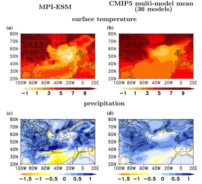
The model shows good agreement with the CMIP5 ensem- ble mean in terms of the simulated surface temperature and precipitation response (Fig. 1, pattern correlation for the region shown: 0.95 for surface temperature, 0.83 for precipitation).
We focus on the far future to enhance the signal to noise ratio.
In the context of mid-latitude ocean-atmosphere interactions, this CGCM experiment forms an interesting extreme case, combining two features of interest: On the one hand, the sur- face temperatures are globally strongly increased as a direct response to the high GHG concentrations. On the other hand, the coupled model setup allows feedbacks from the atmos- phere onto the ocean circulation. The thermohaline circulation in the ocean is to large extent driven by water masses cooling down to very low temperature in the high latitudes in boreal winter, leading to deep ocean convection and the formation of North Atlantic Deep Water. The MPI-ESM RCP 8.5 scenario
projection shows a significant slowdown of the AMOC in the future, as well as changes in the gyre circulation in the North Atlantic. These have consequences for the SST gradients. A detailed discussion of the changes in ocean circulation is given in Fischer et al. (2017). For this reason, we will give only a very brief summary on this topic in Sect. 3.1. Following on from Fischer et al. (2017), our main objective of this paper is to better understand the processes controlling the atmospheric response to the changing ocean surface conditions in this
scenario. For this purpose we perform sensitivity experiments with the atmospheric component of the model to partition the atmospheric response to global warming into a part that arises from local SST changes in the North Atlantic (includ- ing, in particular, SST gradient changes in the Gulf Stream region) and a part caused by local large-scale SST changes, remote SST changes, and the direct impact of radiative forcing changes on the atmosphere.
Fig. 1 Winter-time (DJF) surface temperature response (top, in K) and precipitation response (bottom, in mm/day) to the RCP 8.5 scenario for MPI-ESM (left column) and the CMIP5 multi-model
ensemble mean (right column). Climatological differences between the periods from 2050 to 2100 and 1850 to 2005. In panels c and d contours repeat the surface temperature change
2 Models and methods
2.1 Coupled model experiments2.1.1 Historical and RCP 8.5 scenario runs of the Coupled Model Intercomparison Project (CMIP5)
This paper focuses on the response of the MPI-ESM to the RCP8.5 scenario. Here we first make a basic com- parison of this model’s response to that of several other models from the CMIP5. Our analysis covers climatologi- cal winter means of different variables from the historical simulations and two different periods from the RCP 8.5 projection runs. We first look at the historical simulations, which were available from 36 models at the time of our analysis. They cover the period from 1850 to 2005 and were forced with historical radiative forcing, aerosols and chemically active gases, as well as land-use conditions. We analysed winter means of the entire period of the runs (i.e.
1850–2005) to represent the current day climate state. Two of our sensitivity experiments (the experiments ”CTL” and
”CTLPNA”, described in Sect. 2.4) were forced with SST patterns based on the SST climatology from MPI-ESM calculated over this period.
The second experiment was a subsequent projection forced by the IPCC RCP 8.5 scenario (IPCC 2013), which includes estimated pathways of the emissions/concentrations of greenhouse gases, aerosols and chemically active gases, as well as land-use and land-cover changes (Vuuren et al.
2011). We used output from the same 36 models as for the historical experiment to analyse climatological averages of the winters during the period from 2050 to 2100.
Furthermore, we analysed extensions of the RCP 8.5 scenario runs up to the year 2300. The extension was not an essential part of CMIP5 and therefore not performed by all modelling groups. When we did our analysis, we had access to data from eight models. For the extension period the emissions of greenhouse gases were fixed at the level of 2100 for another 50 years, before starting to decline after 2150, leading to a stabilization of the radiative forcing at approx. +12 W/m2. Chemically active gases and land-use are held at the level of the year 2100. We analysed winter climatologies for the period from 2200 to 2300. As we will show later in the results section, the global warming patterns are similar between the more recent and far future periods, but with enhanced amplitude for the far future. For two of our sensitivity experiments (the experiments called ”FULL”
and ”FULLMNA”, for details refer to Sect. 2.4), the SST forcing is based on the SST climatology from MPI-ESM calculated over this period.
The three periods differ in length because they were selected to characterise three different stages of AMOC
evolution. The current stage during which AMOC is rather stable and represents present day conditions (1850-2005), AMOC decline phase (2050-2100), and a collapse or strongly weakened but stable future AMOC phase (2200- 2300). We chose the longest periods possible to character- ise these phases and allow robust estimates of the climatol- ogy. By comparing the two future periods we also show the robustness of the North Atlantic SST global warming response pattern.
In CMIP5 there was also a prioritization of the output variables. Most of the variables we analysed (e.g. precipita- tion and surface temperature) were of the highest priority and therefore available for all runs that we analysed. On the contrary, the baroclinic and the ocean meridional overturn- ing stream function were variables of only medium priority and therefore they were available for only four models for the entire period.
2.1.2 Description of the Max Planck earth system model (MPI‑ESM)
2.2 General model description
First, we analyse a set of transient simulations with the Earth System Model of the Max Planck Institute for Meteorology, Hamburg (MPI-ESM) that were performed for CMIP5. The atmospheric component has a horizontal spectral resolution of T63 (approx. 1.8° × 1.8°) with 47 vertical levels and a top at 0.01 hPa. ECHAM6 includes the land-surface model JSBACH to provide the lower-atmospheric boundary condi- tions over land. For the coupled runs ECHAM is combined with the MPI Ocean Model (MPIOM) with a resolution of GR15L40 (approx. 1.5° horizontal resolution, 40 vertical levels), using the OASIS 3 coupler. Giorgetta et al. (2013) give a detailed model description.
Precipitation is parametrized in the model. For convec- tive precipitation, ECHAM uses the Tiedtke (1989) mass flux scheme with modifications for penetrative convection according Nordeng (1994). The deep convection scheme uses a closure based on convective available potential energy (CAPE), while for shallow convection the closure is based on large-scale moisture convergence. Entrainment and detrainment rates for penetrative convection are also related to CAPE. For large scale precipitation, the model uses a stratiform cloud scheme, which is based on prognos- tic equations for the mixing ratios of the water phases, bulk cloud microphysics (Lohmann and Roeckner 1996) and a statistical cloud cover scheme.
2.3 Performance of MPI‑ESM in simulating the historical climate in the North Atlantic region
The performance of MPI-ESM to reproduce ocean-atmos- phere interaction in the NA sector is assessed by plotting cli- matologies of key quantities from the historical run (suppl.
Fig. S.3, averaged for DJF in the historical run from 1850 to 2005). According observations/reanalysis are provided in the supplements (suppl. Fig. S.4). The latter include satel- lite observations of SST from the NOAA optimal interpola- tion data set (Reynolds et al. 2002), reanalysis data for SLP, 10m- winds and vertical wind speeds from the NCEP-NCAR reanalysis (Kalnay et al. 1996) and satellite-observed pre- cipitation from the Global Precipitation Climatology project (Adler et al. 2003).
As most recent coupled ocean-atmosphere models, MPI- ESM has problems to reproduce a realistic Gulf Stream path (Jungclaus et al. 2013), which are reflected by the SST pat- tern (suppl. Figs S.3a and S.4a). Compared to observations, the separation of the Gulf Stream from the coast is located slightly northward of the observed position. The northward turn at the Grand Banks is not simulated by the model and the path of the North Atlantic current is too zonal.
For the previous version of the model, a detailed analysis of the hydrological cycle has been performed (Hagemann et al. 2006). The precipitation bias patterns remain in the newer model version, but slight improvement has been made concerning the amplitude of the precipitation biases (Ste- vens et al. 2013). ECHAM overestimates global averaged precipitation compared to observations, particularly over the oceans. The strongest biases occur in the tropics, while the model has a much better performance in the mid-latitudes.
Particularly, the model reproduces the Gulf Stream precipi- tation band very well, even though slightly too week (suppl.
Figs. S.3c and S.4c). The precipitation band can be associ- ated to low-level convergence (suppl. Fig. S.3d) and upward motion, penetrating deep into the atmosphere (suppl. Figs.
S.3f and S.3e), supporting previous findings (Minobe et al.
2008). The climatological storm track (suppl. Fig. S.3b) shows good agreement with the NCEP-NCAR reanalysis (suppl. Fig. S.4b).
2.4 Sensitivity experiments
2.4.1 General setup of the sensitivity experiments
We use ECHAM6, the atmospheric component of MPI- ESM, to perform sensitivity experiments designed to decom- pose the global warming response of the atmosphere into a component driven by North Atlantic SST pattern changes (including the location and strength of the Gulf Stream SST front) and a component that covers all other processes. The
latter includes the direct response to changed radiative forc- ing as well as the response to remote SST changes outside the North Atlantic and a homogeneous warming of the North Atlantic. The experiment consists of four runs that differ in terms of their radiative and SST forcing (details in the next paragraph). Each run is 60 years long and uses a monthly varying climatological forcing, which has an annual cycle, but does not differ between the individual years within each run. Since the memory of the atmosphere is usually less than one year, each of the 60 winters in these experiments can be seen as an independent realization with the same forc- ing, which allows us to perform robust statistical tests. Even though the experiments were performed for the entire years, only the winter season was analysed. For all sensitivity runs, we assumed a spin-up time for the atmospheric model of 5 years. Also we dropped the first and the last winter, so that only winters were analysed for which all three month were available, resulting in the analysis of 54 winters.
2.4.2 Forcings for the individual sensitivity experiments Figure 2 illustrates the SST forcing pattern that is referred to in the following description of the setup, averaged over the winter months (DJF, note that the forcing was monthly varying). The contours represent the absolute SST used as forcing in the corresponding run, while the shadings in sub- panels (b–d) are the difference with respect to the control experiment (CTL, details follow). Since the main focus of our analysis was on the North Atlantic region the figure is limited to this region, although SST was prescribed globally.
For the complete global winter-time forcing fields refer to suppl. Fig. S.5.
The control run (CTL) uses averaged radiative forcing and monthly climatologies of the SST from the period 1850 to 2005 from the historical coupled run (Fig. 2a). FULL uses atmospheric forcing and SST boundary conditions from the coupled RCP 8.5 scenario projection run, averaged for the period from 2200 to 2300 (contours in Fig. 2b).
CTLPNA (abbrev. for ”CTL plus North Atlantic SST pat- tern change”, Fig. 2c) isolates the impact of the local North Atlantic SST pattern changes projected for the 23rd century.
For this purpose, a local SST anomaly was added to CTL in the North Atlantic region (25°N to 66°N). The anomaly (shadings in Fig. 2c) was chosen to represent that part of the SST change, which is likely mainly caused by ocean circula- tion changes in the North Atlantic region, even though by our design we cannot fully exclude that also other processes, such as changes in surface heat fluxes, may contribute to it.
It was created by taking the difference between FULL and CTL (shadings in Fig. 2b) and then subtracting a spatially homogeneous offset; that offset is the globally averaged SST change between 2200-2300 and 1850-2005. The resulting pattern shows a relative cooling of the North Atlantic, likely
as a result of a AMOC slowdown by approximately 50% in the coupled experiment [suppl. Fig. S.2, and Fischer et al.
(2017)]. Furthermore it includes a relative cooling of the southern side of the Gulf Stream region in the historical run and a relative warming north of it, likely as a result of a northward shift of the Gulf Stream axis in the coupled experiment. The radiative forcing and the SST outside the North Atlantic are the same as in CTL. Therefore, CTLPNA excludes all other aspects of global warming, i.e. the direct response to the changed radiative forcing and large-scale warming and the impact of SST changes in remote ocean regions.
FULLMNA (abbrev. for ”FULL minus North Atlantic SST pattern change”, Fig. 2d) assesses the impact of all those global warming related aspects that were excluded in CTLPNA, but neglects the effects from local SST pattern changes. To compute the SST forcing for the North Atlantic, the same local SST anomaly was subtracted from FULL, that
was added to CTL to generate CTLPNA (see last paragraph for a definition of this anomaly). For the North Atlantic between 31°N and 60°N the remaining SST difference with respect to CTL by definition is a homogeneous warming by the globally averaged SST change between 1850-2005 and 2200-2300 (shadings in Fig. 2d), meaning that the spatial structure of the local SST pattern from CTL is conserved (as can be seen by comparing the contours in Fig. 2d and a).
The radiative forcing are the same as in FULL and outside the North Atlantic the SST is identical to that in FULL.
In CTLPNA and FULLMNA the northern and south- ern edges of the anomalous SST pattern that was added (CTLPNA)/subtracted (FULLMNA) were smoothed to avoid artificial gradients. Therefore, the anomaly was mul- tiplied by a weighting factor, increasing linearly from 0 to 1 in 6°-wide latitude bands (i.e. 25°N to 31°N and 60°N to 66°N).
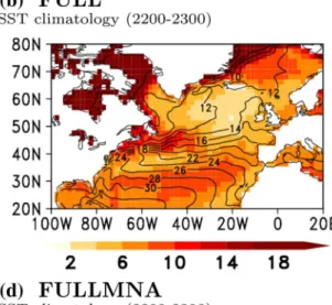
Fig. 2 Winter-time SST forcing for the sensitivity experiment. The contours show absolute SSTs (in °C) for each run, averaged for the winter months (DJF) for CTL (a), FULL (b), CTLPNA (c) and FULLMNA (d). In panels b–d the shadings are the SST difference
(in K) with respect to CTL. For details on the local SST anomaly that was added to CTL in c/subtracted from FULL in d in the region 25°N to 66°N (the region between the green lines) refer to Sect. 2.4.2
For all runs, the sea ice forcing was generated, by assum- ing all regions to be ice-covered (ice-free) where adding the SST anomaly results in SSTs colder (warmer) than −1.8°C.
2.5 Analysis methods
To obtain a deeper understanding of the mechanisms that control precipitation changes in our experiments, in Sect. 3.2.1 we present a moisture budget analysis, follow- ing the method used in Seager et al. (2010). The idea of the method is to disentangle the moisture transport changes into contributions that can be related to different physical processes. Here, we will only give a very short summary of the method, for a more detailed description refer to Seager et al. (2010) and Seager et al. (2014). We start from the following equation for the P–E imbalance:
where 𝜚w represents the density of water, g the accelera- tion due to gravity, and 𝛿(P−E) the change in precipitation minus evaporation. The terms on the right hand side are
and
p is the pressure, 𝐮 the horizontal wind vector and q the specific humidity. Primes indicate fluctuations on sub- monthly timescales, xref the climatological mean of the quantity x in the unperturbed reference run, 𝛿(x) stands for the difference of the climatological means of the quantity x between the perturbed run and the reference run, and
∇⋅() is the horizontal divergence of a quantity. Subscript s indicates surface quantities. The physical meaning of the terms on the right hand side is as follows: 𝛿TH represents thermodynamically induced changes, i.e. changes that are related to the changed climatological moisture concentra- tion in the perturbed run with respect to the reference run, assuming that the circulation is held fixed at the value of the reference run. 𝛿MCD represents these changes that are due to changes in the climatological mean circulation of the atmosphere, holding the moisture concentrations (1) 𝜚wg𝛿(P−E) ≈𝛿TH+𝛿MCD+𝛿TE−𝛿S−𝛿NL,
(2) 𝛿TH = −
∫
ps
0
∇⋅(𝐮ref[ 𝛿q]
)dp,
(3) 𝛿MCD= −∫
ps 0
∇⋅([ 𝛿𝐮]
qref)dp,
(4) 𝛿TE= −
∫
ps
0
∇⋅𝛿(𝐮�𝐪�)dp,
(5) 𝛿S=𝛿(qs𝐮s⋅∇ps),
(6) 𝛿NL= −
∫
ps
0
∇⋅(𝛿u𝛿q).
fixed at the concentration of the reference run, i.e., mois- ture convergence due only to changes in the convergences and divergences of the climatological mean wind field.
𝛿TE includes the changes in moisture flux convergences and divergences on sub-monthly time scales, mainly from transient eddies on synoptic timescales. 𝛿S accounts for changed gradients in the climatologically averaged surface pressure field (setting the lower boundary for the vertical integrals), and 𝛿NL is a nonlinear term, accounting for correlated changes in both, the climatologically averaged wind and moisture fields.
We use a bootstrapping method to test the time mean difference of a quantity 𝜙(x,t) in a perturbed experiment P and the same quantity in a reference experiment R on its significance. Let < 𝜙P(x)> be the time average of 𝜙 over all winters in experiment P and let < 𝜙R(x)> be the time average of 𝜙 over all winters in experiment R. The null hypothesis is that < 𝜙P(x)> and < 𝜙R(x)> are not different, considering the year-to-year variability of the winter-time averages of 𝜙 . To reject the null hypothesis, we use the time series of annual winter means of 𝜙 for 54 winters from each run. Each winter of each experiment is treated as independent realizations under the same forcing.
We create 1000 resamples (with replacement) from 𝜙P(x,t) and 𝜙R(x,t) and then compute the difference of the means for each pair of resampled time series to estimate the 95%
quantile Q95(x).
3 Results
3.1 Simulated local response of the coupled model in the CMIP5 context
In this section, we will describe the winter-time temperature and precipitation response to the RCP 8.5 scenario in MPI- ESM and compare it to other CMIP5 models. A brief discus- sion is provided on the link to ocean circulation, for a more detailed discussion on the ocean changes refer to Fischer et al. (2017). It is likely that large-scale changes in the ocean circulation drive the SST changes (Drijfhout et al. 2012).
However, part of the pattern may be driven by changed heat fluxes from the atmosphere into the ocean.
For the period from 2050 to 2100 the temperature and precipitation responses to the RCP 8.5 scenario simulated by MPI-ESM are in agreement with the CMIP5 multi-model ensemble mean (Fig. 1). For the far future (2200 to 2300, Fig. 3) the shape of the patterns remain the same, but the amplitude of the signal is strongly enhanced. The pattern correlation between the two periods is 0.96 for surface tem- perature and 0.88 for precipitation. The signal is dominated by a strong warming over the entire North Atlantic, but the pattern shows distinct regional differences. In agreement
with the CMIP5 ensemble mean, MPI-ESM shows a local minimum of the warming in the north east North Atlantic and a local maximum in the region of the Grand Banks.
Comparing those models with RCP8.5 runs extending to 2300 (i.e. eight models) shows a first order agreement in the simulated temperature response (suppl. Fig. S.6). Con- tinents in general warm more strongly than the oceans, and most models show a local minimum in the northern North Atlantic, that is also clearly visible in the multi-model ensemble mean. This so-called ”warming hole” has been connected to a slowdown of the Atlantic Meridional Over- turning Circulation that is a common feature of long-term climate projections with strong radiative forcing (IPCC 2013, Ch. 12). Following Fig. 12.35 from the IPCC 5th Assessment report, we show the AMOC time series in suppl. Fig. S.2, but at a more northern latitude. For the period until 2300 data for the AMOC were only available for four models, but these agree in simulating a substantial weakening of the overturning. In MPI-ESM, the decline is more than 50% of the average AMOC during the historical
period. After reaching a minimum around the end of the 22th century, there are indications for a recovery of the AMOC in our model.
The response among models, however, differs in some details. The position of the local SST minimum described in the last paragraph varies from model to model. This might be related to differences in the structure of the subpolar gyre and related changes (suppl. Fig. S.7). A common feature for those models where data for the barotropic stream function were available is a northward shift of the boundary between subpolar and subtropical gyre, which in the RCP 8.5 projec- tions consistently lies at a position at approx. 50 to 52°N for the period from 2200 to 2300.
Beyond this, some of the models show other local fea- tures. In MPI-ESM a strong warming along the Canadian coast and over the Grand Banks is flanked to the south by a zonally oriented band of only moderate warming in the region of the Gulf Stream and its extension (approx. 70°W to 40°W, 35°N to 40°N). Some models (CSIRO-Mk3-6-0, IPSL-CM5A-LR and CNRM-CM5) show a similar feature,
(a)
(c)
(b)
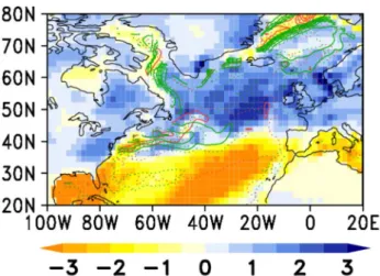
Fig. 3 Winter-time surface temperature response (a, in K), the abso- lute value of the SST gradient (b, in K/100km) and precipitation response (c, in mm/day) to the RCP 8.5 scenario in MPI-ESM. Cli-
matological differences between the periods from 2200 to 2300 and 1850 to 2005. Underlying contours in b) show the annual mean SST for the RCP 8.5 scenario run in the period 2200-2300
but the exact shape and position of this local minimum in the warming varies. We suggest, that this local structure is con- nected to changes in the gyre circulation: In MPI-ESM there is a slight northward shift of the ocean currents south of Newfoundland, as indicated by the barotropic stream func- tion (suppl. Fig. S.7a). A similar feature can be found in CSIRO-Mk3-6-0 (suppl. Fig. S.7d), which consistently also shows a band of reduced warming there (suppl. Fig. S.6d).
Concerning the precipitation response (Fig. 3c and suppl.
Fig. S.8) models agree in simulating a drying over the sub- tropical eastern North Atlantic and North Africa and the Mediterranean region. Increased precipitation is found north of it, over the mid-latitude North Atlantic, middle and north- ern Europe and northern North America. The precipitation response in the western subtropical Atlantic varies greatly among the models. In the region where the individual mod- els simulate the ”warming hole” discussed in the previous paragraph, the increase in local precipitation is (partly) sup- pressed. In some of the models (i.e. CCSM4, CNRM-CM5 and GISS-E2) this causes even a decrease in local precipita- tions, while in the others the increase is only reduced with respect to the surrounding regions.
In MPI-ESM the response furthermore includes a zonally banded dipole structure with heavily enhanced precipitation south and south-east of Newfoundland, flanked by a region on the southern side of the historical Gulf Stream SST front that becomes dryer (Fig. 3c). This feature is only found in some models, i.e. IPSL-CM5A-LR (suppl. Fig. S.8g) and CSIRO-Mk3-6-0 (suppl. Fig. S.8d), which also have a similarly structured temperature response here. The drying is contrary to the usual expectation that wet regions will become wetter and dry regions drier in a warmer climate (IPCC 2013; Held and Soden 2006). This indicates that the precipitation changes are not exclusively related to a higher moisture content of the atmosphere due to the warming, but there must also be changes in the atmospheric circulation.
Precipitation in the Gulf Stream region has been linked to the SST gradient in that region [e.g Minobe et al. (2008)].
Therefore it is likely that the modulation of the precipita- tion response is connected to SST gradient changes as well, rather than to absolute SST alone. In the historical simula- tion of MPI-ESM, strong meridional gradients in surface temperature are located at the Gulf Stream front (suppl. Fig.
S.9a). The most prominent feature of the projected future changes of the SST gradient, is a weakening of the SST gradient in the region of the historical Gulf Stream front (Fig. 3b). However, this region remains the region with the strongest meridional SST gradients in the future projection (suppl. Fig. S.9b), albeit values are reduced by up to 50%
with respect to the historical run. North of the area with
reduced gradients we find a region with enhanced gradients east of Newfoundland.
Another region of both, strong surface temperature and surface temperature gradient changes is found in the high latitudes. This is related to the fact that sea ice in the Arc- tic has completely melted in the future simulations (suppl.
Fig. S.5). While surface temperature refers to the very cold surface temperature of the ice cover in the historical simu- lation, it means the temperature of open ocean in the RCP 8.5 projections. It has to be considered that these changes also contribute to the climate change response in the high latitudes. Here we are mainly interested in the effect of SST changes arising from differences in the mid-latitude ocean circulation of the North Atlantic. For this reason we deliber- ately excluded the region north of 66°N from the modifica- tions to the SST forcing pattern to disentangle the influence of local SST pattern changes from other factors, described next. In other words: What we will refer to as ”response to local SST pattern changes” from now on, does not include the effects of melted sea ice in the Arctic1.
3.2 Sensitivity experiments to assess the impact of local SST changes in the North Atlantic sector Our hypothesis is that the dynamical changes, suggested by the analysis in the previous section, can be linked to local SST pattern changes in the North Atlantic. We perform experiments with the atmospheric model component to iso- late the impact of the SST changes; a detailed description of the experimental setup is given in Sect. 2.4.
3.2.1 Response of the local atmosphere
We start with a description of the precipitation response in the individual runs, and additionally provide some figures investigating the related atmospheric circulation.
Figure 4a and b show the winter-time seasonal mean precipitation response in the sensitivity experiments with respect to the control experiment (CTL). First, we started to compare FULL, a run performed with climatological forc- ing from the future scenario coupled run, to CTL, forced with the climatological conditions from the historical run.
The idea of this experiment is, to verify that it is possible to reproduce the main features of the precipitation response in the coupled run with climatological forcing factors and an
1 Note that there is a very small region, for which this statement does not fully hold: In the Labrador Sea, along the coast of Canada there is a region where the sea ice extends far to the south in the historical simulations. This region is modified by the SST anomaly added/sub- tracted in CTLPNA/FULLMNA. In this region our SST modification indeed artificially melts some sea ice. We believe this to play a minor role, since the sea ice was basically orientated in a small band along the coast where there would be a strong surface temperature gradient due to the land-sea contrast anyway.
atmosphere-only setup. Indeed, in terms of total precipita- tion, FULL reproduces the winter-time precipitation changes from the coupled transient experiment well (Figs. 3c and 4a). Subtle differences can be found in the amplitude of the response, with the sensitivity experiment showing a slightly stronger response than the coupled model system. This is likely to be explained by the atmosphere-only setup con- figuration that lacks a negative feedback; in the sensitivity experiments there is no cooling effect on SST by enhanced evaporation and reduced radiative fluxes that usually occur with enhanced cloud-cover and precipitation. The strongest precipitation increase in the experiment with the full future
conditions (FULL) occurs southeast of Newfoundland, where the northward shifted Gulf Stream causes a strong SST warming (Fig. 2b) and strongly enhanced meridional SST gradients (Fig. 3b). In the region of the southern flank of the historical Gulf Stream front (approx. 33°N to 39°N and 70°W to 40°W) precipitation decreases, even though SSTs are slightly increased. Also, as described in the previ- ous section, this is a region where we find wet conditions in present-day climate. Therefore these precipitation changes are likely due to the changes in the SST gradient.
Now, we separate the SST forcing into a mean warm- ing and local pattern changes in the North Atlantic: In the
Fig. 4 Winter-time total precipitation response (in mm/day) in the sensitivity experiments. Plotted are climatological differences in FULL (a), CTLPNA (b) and FULLMNA (c) with respect to CTL and climatological difference of FULL with respect to FULLMNA (d).
Non-significant values (at the 95% confidence level, based on a boot- strapping test) are masked. Contours in c and d indicate the change in the SST gradient (contour interval 0.5 K/100 km, negative values are dashed.)
FULLMNA experiment we consider the effects resulting from a homogeneous warming of the North Atlantic (con- serving the shape SST of the local SST pattern, but adding a constant temperature offset), changed radiative forcing, and remote SST changes outside the North Atlantic (Fig. 2d).
FULLMNA reproduces the gross changes in precipitation across the North Atlantic, with a wetter extra-tropics and drier subtropics (Fig. 4b). However, there are key differences to the FULL response. These include stronger precipitation changes west of the British Isles (Fig. 4b). Furthermore, the structure of the local response pattern in the Gulf Stream region, particularly the drying found in the coupled experi- ment and in FULL, is not reproduced in this experiment.
In contrast, the experiment with local pattern changes (CTLPNA, Fig. 4c) reproduces this drying. This supports our hypothesis that this feature is primarily driven by local SST gradient changes. Furthermore, we find an extended drying of the north eastern Atlantic basin (Fig. 4c), where the absolute SST shows a distinct cooling that is likely a result of the AMOC slowdown. In this case, we assume the absolute SST to be the driving factor for the precipitation change.
For analysis of the linearity of the response and to inves- tigate the effects from a changed atmospheric background state due to changed radiative forcing, we also included a comparison between FULL and FULLMNA (Fig. 4d). The pattern shows high similarity to that from CTLPNA minus CTL (Fig. 4c), except that the same SST gradient change causes an enhanced amplitude of the pattern in a warmer background state.
The local response to the SST pattern change in the Gulf Stream region is associated with a zonally orientated dipole structure in the low-level wind convergence (Fig. 5b) and the vertical wind field (Fig. 5d and f). The low-level con- vergence and the vertical motion is intensified in the north, and weakened south of the position of the historical SST front. This pattern is consistent to the structure of the SST gradient changes in this region, as well as with the precipita- tion changes. For the case with the homogeneous warming (Fig. 5a, c and e) these changes are absent.
To better understand the mechanisms contributing to precipitation changes in the North Atlantic region, we per- formed an analysis of the local moisture budget. For conti- nuity reasons, in the long-term mean precipitation changes have to be balanced by the sum of the changes in local evaporation and changes in the vertically integrated local moisture flux convergence/divergence.
The local evaporation response field shows a structure that is, to a first approximation, similar to the precipitation response (Fig. 6a). This raises the question what causes the local evaporation changes. In ECHAM6, the atmos- pheric component of MPI-ESM, the surface flux of specific
humidity over the ocean is approximated by the following bulk formula:
where − C is a bulk coefficient (for details see chapter 2.4 of Giorgetta et al. 2013), 𝐕 is the absolute value of the dif- ference between the surface velocity and the wind velocity at the lowest model level, qnlev is the specific humidity at the lowest model level and qsfc surface specific humidity.
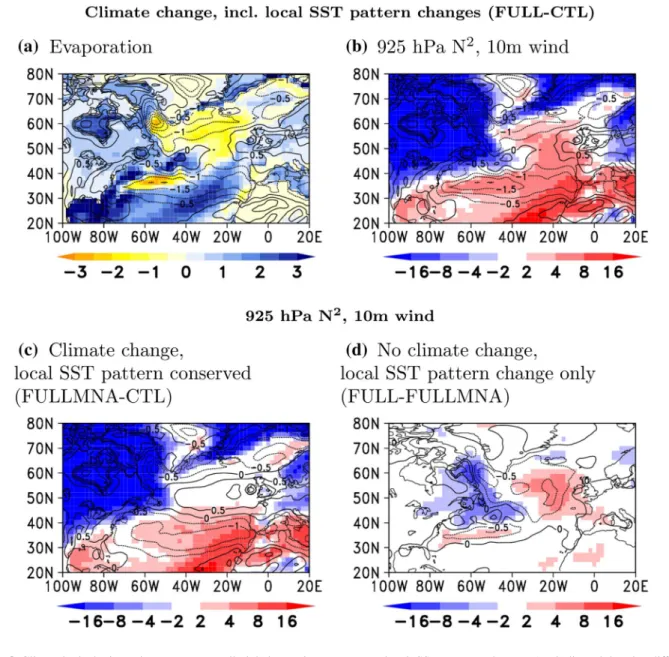
We anticipate that changes in wind speed drive the reduc- tion in evaporation, as wind speed generally dominates vari- ations in evaporation over the extra-tropical oceans. Indeed the changes in 10m wind speed show a very similar structure to the evaporation change in many regions, particularly over the western part of the ocean basin (Fig. 6a). The structure of the wind change at the 925 hPa pressure level looks slightly different (not shown) and shows more similarity to the sur- face wind speed changes related to homogeneous warm- ing (Fig. 6c). We suggest that a reduced downward mixing of momentum as a result of a locally stabilized boundary layer in the region of the reduced evaporation is involved in controlling the wind speed changes, and hence the local reduction in evaporation. This hypothesis is supported by the congruent enhancement of low-level static stability, as indicated by the squared Brunt-Väisälä frequency (Fig. 6b).
In general, under global warming the marine boundary layer is stabilized (Fig. 6c), consistent with a more moderate warming over the ocean compared to land. The stabiliza- tion goes along with a large-scale reduction in surface wind speed, except in the region between 45°North and 60°North, where the enhanced wind speed is likely related to changes in storminess along the North Atlantic storm track, which will be discussed in Sect. 3.2.2. In addition to the large-scale stabilization and surface wind reduction the weakening of the SST front regionally leads to very localized further sta- bilization and surface wind reduction (Fig. 6d). In the region of the weakening of the evaporation these two overlying effects then allow the resulting surface wind speed changes to become large enough to overcompensate the countering temperature related large-scale evaporation enhancement.
Although evaporation is capable to explain a large part of the precipitation change in many regions, there is still a noteworthy imbalance in the precipitation minus evapora- tion change (Fig. 7), that needs to be explained by changes in moisture transport convergence. For this purpose we per- formed an analysis of the changes in the vertically integrated moisture flux convergences and divergences, following the method by Seager et al. (2010). The method disentangles the moisture transport changes into contributions that can be related to different physical processes. A brief descrip- tion of the method is provided in the methods section of this
(7) w�q�sfc= −C|𝐕|(qnlev−qsfc),
Fig. 5 Winter-time response of the 10m-wind convergence (top, in 10−6 /s), the vertical wind at 850 hPa (middle, in Pa/s, red denotes a strengthening of the upward direction) and vertical cross sec- tions (bottom) of the vertical wind response (in Pa/s, red denotes a strengthening of the upward direction) and the horizontal wind con- vergence (contours, in 10−6 s−1, negative values are dashed) zonally
averaged between 65°W and 50°W (the region indicated by the box in c and d). As before, the left column shows the response to homo- geneous warming and the changed background state and the right col- umn the response to local SST pattern changes. In subfigures a to d non-significant values (based on a bootstrapping test at the 95% confi- dence level) are masked
paper, for a more detailed description refer to Seager et al.
(2010, 2014).
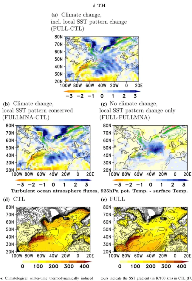
First, we look at the thermodynamically induced changes in the vertically integrated moisture flux convergence 𝛿TH . This term can be understood as the effects that arise from (thermodynamically induced) changes of the moisture field, when the circulation is held fixed at the conditions in the reference run. In the full response, 𝛿TH plays a domi- nant role in the region along the US east coast (Fig. 8a).
In winter the continents are much colder than the ocean at the same latitude, which causes strong upward turbulent ocean-atmosphere fluxes and large difference between the
925 hPa temperature and the (prescribed) temperature of the surface, when the cold air is advected towards the marine region (Fig. 8d, e). One can look on an air parcel from a Lagrangian perspective, following it on its way with the mean eastward flow: As soon as the air parcel reaches the coast, the ocean starts warming it at the surface by strong sensible heat fluxes. It is worth to mention, that since we use a prescribed SST setup, the SST can not respond to the atmosphere. The warmer the air parcel becomes, the more moisture it is able to carry. From an Eulerian perspective this means for an individual grid cell close to the coast, that the air entering it from the west is usually colder and contains
Fig. 6 a, b Climatological winter-time response to all global warming related changes in the forcing (as indicated by the difference between FULL and CTL) for evaporation (a, shadings, in mm/day) and low- level static stability, indicated by the squared 925 hPa Brunt-Väisälä frequency (b, shadings, in 10−2 /s) and 10m-wind speeds (contours, in m/s). c, d Same as b, but for the response to all forcing changes
except local SST pattern changes (as indicated by the difference between FULLMNA and CTL, c) and response to local SST pat- tern changes only (as indicated by the difference between FULL and FULLMNA, d). In all subfigures non-significant values (based on a bootstrapping test at the 95% confidence level) are masked
less moisture than the air leaving it to the east. This leads to a net moisture flux divergence and therefore compensates much of the strong evaporation that occurs in this region. It has to be considered, that the direct warming effect of the radiative forcing in general leads to larger warming over land than over the ocean. Nevertheless there is only little difference in the coastal ocean-atmosphere turbulent fluxes between CTL and FULL (Fig. 8d, e), indicating that the seasonal land-sea temperature contrast is the dominant fea- ture compared to the differential response to global warm- ing. We did not explicitly compute the heating rates in the atmosphere caused by the turbulent ocean-atmosphere fluxes in the coastal region, but it appears plausible to assume that they are of similar magnitude for both runs. According to the Clausius-Clapeyron equation the increase in saturation water Es vapour pressure is not linear, but under high tem- peratures a warming by a specific temperature difference 𝛿T will cause a larger change in the saturation water vapour pressure 𝛿Es than for the same 𝛿T under cold conditions. As a result similar heating rates from the air -sea fluxes would lead to the enhanced thermodynamically induced moisture flux divergence 𝛿TH under warm than under cold condi- tions and therefore likely cause the more divergent coastal moisture flux in the full response. This argumentation is sup- ported by the fact that the divergent response 𝛿TH close to the coast is not present, when considering the differences between runs that do not differ in terms of radiative forcing, but only in the local SST pattern (i.e. FULL-FULLMNA, Fig. 8c). A convergent moisture flux response around 60°W related to the local SST pattern change (Fig. 8c) compen- sates the convergent response to the large-scale warming in this region (Fig. 8b), resulting in a shrinking of the region
with a divergent response when considering all forcings (Fig. 8b).
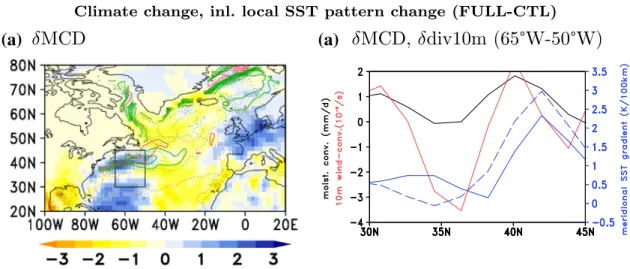
𝛿MCD represents the changes in the vertically integrated moisture flux convergence, that are related to changes in the climatological mean circulation. This term partly com- pensates with the effect of atmospheric eddies in the region of the SST front (see Figs. 9a and 10 and next paragraph).
Because a large part of the moisture is concentrated in the lower levels of the atmosphere, the response of the con- vergence of surface winds shows good agreement with the change in moisture flux convergence (red and black line in Fig. 9b). As shown before (comparison between the left and the right column of Fig. 5) the dipole-like structure of the local circulation response is nearly exclusively driven by the changes in the local SST pattern rather than by the large-scale changes. The same holds for 𝛿MCD : The full response of the circulation induced change in moisture flux convergence (upper row of Fig. 9) closely resembles the part that arises from the local SST pattern change (lower row of Fig. 9) and the according response in low-level wind conver- gence (Fig. 5b and f). In comparison to the latter, the local response of 𝛿MCD is small and does not show the dipole-like structure when conserving the SST pattern (middle row of Fig. 9).
Beside this, the moisture budget includes contribu- tions from three more terms: 𝛿TE , represents effects due to changes in the eddy moisture flux convergence and will be discussed in context with the storm-track changes in the next section. The non-linear term 𝛿NL , accounting for cor- related changes in the moisture and wind-fields, becomes non-negligible when comparing runs with strong tempera- ture differences (suppl. Fig. S.10a and S.10d) and has some similarity with the climatological precipitation field (suppl.
Fig. S.3c for the historical coupled run), indicating that changes in the moisture gradients are linked with changes in the atmospheric circulation there. As a possible explana- tion, we speculate that enhancing the moisture content of the atmosphere due to warmer conditions might influence the atmospheric circulation by offering an additional latent heating source in regions with strong precipitation. The additional heating then could accelerate the upward motion and hence for continuity enhance low-level convergence, resulting in a stronger moisture flux convergence, providing a positive feedback.
Finally, we have to acknowledge that we could not fully close the moisture budget with the method described in this paragraph (suppl. Fig. S.10), but there is a non-negligible residual. For the local SST pattern change related response, the residual (suppl. Fig. S.10i) shows similarity to the eddy term 𝛿TE (Fig. 10c). This might be seen as an indicator, that taking 6-hourly output, as we did, misses a noticeable part of the eddy moisture transport, and therefore may explain the the residual in our analysis. Furthermore, 𝛿S shows high
Fig. 7 Climatological winter-time difference between FULL and CTL for the precipitation minus evaporation imbalance (shadings, in mm/
day). As indicator for the position of the SST front, the absolute value of the SST gradients (in K/100 km) in both runs are shown as green (for CTL) and red (for FULL) contours. Solid contours represent steps of 1K, dashed contours the 1/2 K steps in between
Fig. 8 a–c Climatological winter-time thermodynamically induced change in the vertically integrated moisture flux convergence 𝛿TH (shadings, in mm/day). Response to all forcings (FULL-CTL, a), all forcings except local SST pattern changes (FULLMNA-CTL, b) local SST pattern change only (FULL-FULLMNA, c). Green (red) con-
tours indicate the SST gradient (in K/100 km) in CTL (FULL). d, e Turbulent ocean atmosphere fluxes (shadings, in W/m2) in CTL (d) and FULL (e) and according differences between 925 hPa potential temperature and 2 m temperature (contours, in m/s, negative values dashed, contour interval 1 m/s
(a) (a)
(c) (d)
(e) (f)
Fig. 9 Left column: climatological winter-time difference for the cir- culation induced response in the vertically integrated moisture flux convergence 𝛿MCD (shadings, in mm/day). Green (red) contours indicate the SST gradient (in K/100 km) in CTL (FULL). Right col- umn: cross-section (zonally average between 65°W and 50°W, indi- cated by the box in the figures in the left column, the same region as in Fig. 5e, f) of 𝛿MCD (black, in mm/day), and the response of the
10-m wind convergence (red, in 10−6 /s). In the panels of the right column the solid (dashed) blue lines represents the zonally averaged meridional component of the SST gradient (in mm/day) in FULL (CTL). Response to all forcings (FULL-CTL, a, b), all forcings except local SST pattern changes (FULLMNA-CTL, c, d) and local SST pattern change only (FULL-FULLMNA, e, f)
values along some coast-lines, particularly when comparing runs with strong temperature difference (suppl. Figs. S.10b and S.10e). This may be related to the high numerical errors in regions with strong gradients, when approximating the derivatives by centered differences, as we did.
3.2.2 Response of the North Atlantic storm track
Changes in surface baroclinicity might modify the storm track (Nakamura et al. 2004) with consequences for the extra-tropical cyclones passing the region, moving towards Europe. Therefore we analysed the response of the North Atlantic storm track in our experiments.
The storminess response in the coupled experiment is weak compared to the climatological values, except for the American continent (and near its coast) and the north-eastern
Atlantic east of 20°W (Fig. 11a). Over America a reduction along the center of the climatological storm track is found.
Enhanced storminess can be found towards the eastern end of the storm track over the northern North Sea, consistent with the findings from Woollings et al. (2012). The cyclones are usually associated with atmospheric cold and warm fronts on their southern side that cause the major part of pre- cipitation in this region (Catto et al. 2012). The precipitation changes west of the British Isles therefore are likely linked to the enhanced storm track slightly north of this region.
The storminess response in the sensitivity experiment is slightly different from that in the coupled model (Fig. 11b).
Especially the strongly reduced storminess over he Ameri- can continent is not reproduced by the atmosphere-only model. Also, the enhancement of the storm track that occurs over the North Sea and north-western Europe in the coupled
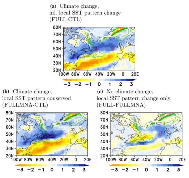
Fig. 10 Climatological winter-time eddy induced change in the ver- tically integrated moisture flux convergence 𝛿TE (shadings, in mm/
day). Response to all forcings (FULL-CTL, a), all forcings except
local SST pattern changes (FULLMNA-CTL, b) and local SST pat- tern change only (FULL-FULLMNA, c). Green (red) contours indi- cate the SST gradient (in K/100 km) in CTL (FULL)
model is much further to the west in the AGCM. We did not further investigate the cause of the discrepancy between the coupled and uncoupled models, but we suggest two plausi- ble reasons. Firstly, the AGCM simulation lacks any feed- back between the storminess and the ocean (e.g through the connection between wind speed and surface turbulent heat fluxes). The wind-driven ocean circulation might adjust to storminess changes in the coupled system, while there is no response of the ocean to changes in the wind field in the AGCM experiment. Second, we force our AGCM with climatological SSTs, and therefore neglect the impact of other SST variability simulated by the coupled model. For example it was shown that ENSO has a significant impact on cyclone activity in the North Atlantic (Merkel and Latif 2002; Fraedrich and Müller 1992). The remote response to any non-linearity between the ENSO phases cannot be repro- duced when using climatologically averaged SST. Therefore, this also might be part of the explanation for the the differ- ences between coupled and un-coupled model, especially over North America.
The sensitivity experiment indicate that in the atmos- phere-only setup the storm track changes in most regions are mainly associated with uniform warming and the direct atmospheric response to the changed radiative forcings (Fig. 11c). The contribution of local SST pattern changes is only significant in the North-eastern Atlantic (Fig. 11d).
Large-scale warming causes enhanced baroclinicity in the high latitude marine regions. (Fig. 11e). South of 50°N there are some regions over the oceans, where local low- level baroclinicity changes are furthermore influenced by local SST pattern changes. However, these changes seem to have no significant impact on local storminess in most of the region. An exception is the region of enhanced baro- clinicity between 30°W and 20°W (Fig. 11f) that may have a small contribution to the SST pattern change induced change of storminess in that region. The latter may be related to a stronger east-west temperature gradient in the simulated future climate at the edge of the ”warming hole” (Fig. 3a, b).
The atmospheric eddies transport moisture and therefore have to be considered in the moisture budget analysis. In our experiments, the term 𝛿TE represents a combination of two effects (Fig. 10): on the one hand, the large-scale warming and the direct response to changed radiative forcing leads to a dipole structure in 𝛿TE , with enhanced convergence (divergence) of eddy moisture fluxes to the North (South) (Fig. 10b). This dipole structure also dominates the full response (Fig. 10a) in most of the North Atlantic region. In the region of the Gulf Stream SST front there is a regionally more convergent eddy moisture flux that is related to the changes in the local SST fields (Fig. 10c). Since this feature falls in the region located just in between the poles of the large-scale dipole structure, it is of regional importance and clearly visible in the full response (Fig. 10). We suggest the following explanation: Eddies that pass along the SST front will lead to cross-frontal winds in both directions, blowing from the north to the south (and hence from the cold side of the SST front to the warm side) on their western side and vice versa on the eastern side. Since the air flowing in the north-south direction on the western side is usually much colder and hence drier than that one flowing in the oppo- site direction, the net effect of the eddies is a cross-frontal moisture transport, resulting in a moisture flux convergence to the north of the front, and a divergence to the south. This mechanism works more efficiently for more pronounced SST gradients. Another factor might be that the strength of the SST front itself might be relevant for empowering the eddies by maintaining the surface baroclinicity (Nakamura et al.
2004).
4 Summary and discussion
Analysis of the coupled MPI-ESM experiment forced with the RCP 8.5 scenario shows a band of intensified winter-time precipitation crossing the North Atlantic from the region south of Newfoundland towards the British Isles. This pat- tern is a robust feature of the CMIP5 multi-model ensemble mean (IPCC 2013, ch.12). In MPI-ESM, this band is flanked to the south by a region becoming drier. This region cor- responds to the southern flank of the historical Gulf Stream extension SST front.
The sensitivity experiments driven by climatological boundary conditions from the coupled experiments can reproduce the precipitation response to the RCP 8.5 sce- nario that was found in the coupled experiment quite well.
The only difference is a slight overestimation of the ampli- tude of the response in the sensitivity experiment, which can be explained by the fact that a negative feedback between SST and precipitation by setup cannot be reproduced in an atmosphere-only setup, as stated in Sect. 3.2.1. However, the
Fig. 11 a–c Climatological winter-time (DJF) storminess response as indicated by the 2-6 day bandpass-filtered anomalies of sea level pressure (in hPa). a Difference between the RCP 8.5 coupled run (averaged for the period 2200 to 2300) and the historical run (aver- aged and averaged for the period 1850 to 2005). b–e Same as a, but for the sensitivity experiment: b difference between FULL and CTL (i.e. the response to all forcing changes), c between FULLMNA and CTL (i.e.the response to all forcing changes except local SST pattern change) and d between FULL and FULLMNA (i.e. the effect of local SST pattern changes only). e, f response of Surface baroclinicity as indicated by the 1000 hPa maximum Eady growth rates (in 10−7 /s).
In (a) the contours show the climatological storminess averaged for the historical run, and in b they indicate the climatological stormi- ness of the CTL experiment. In subfigures b–f non-significant val- ues (based on a bootstrapping test at the 95% confidence level) are masked
◂