Short Course SC1.1
Data assimilation in the geosciences – Practical data assimilation
with the Parallel Data Assimilation Framework
Lars Nerger 1 , Maria Broadbridge 2 ,
Gernot Geppert 3 , Peter Jan van Leeuwen 2,4
1: Alfred Wegener Institute, Bremerhaven, Germany 2: University of Reading, UK
3: Deutscher Wetterdienst (DWD), Offenbach, Germany 4: Colorado State University, Fort Collins, CO, USA
EGU General Assembly 2019
SC1.1: Ensemble Data Assimilation with PDAF
The Short Course – Overview
1. Introduction to ensemble data assimilation 2. Implementation concept of PDAF
(Parallel Data Assimilation Framework) 3. Hands-on Example:
Build an Assimilation System with PDAF
1
Introduction to
Ensemble Data Assimilation
SC1.1: Ensemble Data Assimilation with PDAF
Overview
• What can we expect to achieve with data assimilation?
• What do we need for data assimilation?
• How does ensemble data assimilation work?
• How can we apply ensemble data assimilation?
Please note:
We omit equations of assimilation methods because you can apply PDAF without knowing them
(See Short Course SC1.2 on Friday for methodology)
Application examples
(ocean physics and ocean-biogeochemistry)
SC1.1: Ensemble Data Assimilation with PDAF
• Generally correct, but has errors
• all fields, fluxes on model grid
• Generally correct, but has errors
• incomplete information:
data gaps, some fields
ocean data: mainly surface (satellite) Combine both sources of information
quantitatively by computer algorithm
➜ Data Assimilation
Motivation
Information: Model Information: Observations
Model surface temperature Satellite surface temperature
DA – effect on Temperature (September 2012)
Assimilation (analysis) Free run
RMS (root-mean-square) deviation
Assimilation (analysis) Free run
Assimilate surface
temperature each 12 h Compare assimilated
estimate with assimilated surface temperature data (monthly average)
Reduce RMS deviation and mean deviation (bias)
➜ necessary effect
Mean deviation (observation – model)
SC1.1: Ensemble Data Assimilation with PDAF
Longe-range effect
Example: Assimilate satellite sea surface height data (DOT)
Androsov et al., J. Geodesy, (2019) 93:141–157
Improve also temperature at 2000m depth
Reduce difference to assimilated
data (necessary)
Assimilation Free – Assimilation
Biogeochemistry: Coupled data assimilation effect
Free run
Surface oxygen mean for May 2012 (as mmol O / m 3 )
Free run
Coupled data assimilation case: physics and biogeochemistry
• Assimilate satellite sea surface temperature observations
• Assimilation directly changes Oxygen and other biogeochemical
variables (strongly-coupled assimilation)
SC1.1: Ensemble Data Assimilation with PDAF
Improving forecasts
• Very stable 5-days forecasts
• At some point the improvement might break down due to dynamics
ACCEPTED MANUSCRIPT
ACCEPTED MANUSCRIPT
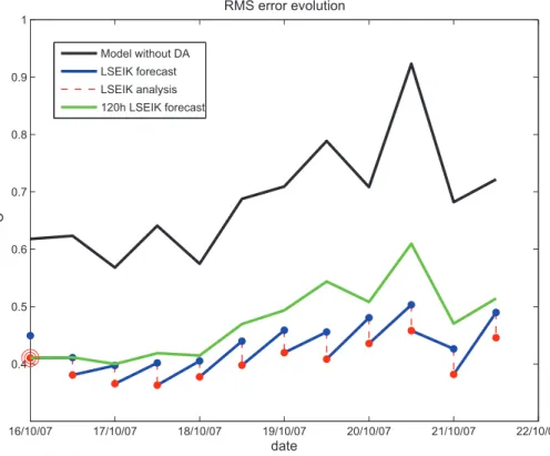
16/10/07 17/10/07 18/10/07 19/10/07 20/10/07 21/10/07 22/10/07
0.4 0.5 0.6 0.7 0.8 0.9 1
date
o C
RMS error evolution
Model without DA LSEIK forecast LSEIK analysis 120h LSEIK forecast
Figure 7: RMS error temporal evolution over the period 16 October 2007 – 21 October 2007 for simulated SST without DA (black curve); LSEIK analysis (red); mean of ensemble forecast based on 12-hourly analysis (blue) and 5 days forecast (green curve) initialized with the analysis state obtained on 16 October 2007.
S. Losa et al., J. Mar. Syst. 105–108 (2012) 152–162
38Impact of Assimilation for temperature forecasts
(North & Baltic Seas)
Bias Estimation
Example: Chlorophyll bias of a biogeochemical model
§ un-biased system:
random fluctuation around true state
§ biased system:
systematic over- and underestimation (common situation with real data)
§ Bias estimation:
Separate random from systematic deviations
Logarithmic bias estimate
April 15, 2004
SC1.1: Ensemble Data Assimilation with PDAF
Estimate a flux (Primary Production)
§ Primary production is a flux: Uptake of carbon by phytoplankton
§ Model: computed as depth-integrated product of growth-rate times Carbon- to-Chlorophyll ratio
§ VGPM: Vertical Generalized
Production model - satellite data only
§ Primary production from assimilation consistent with VGPM-estimate
§ Important: Concentration change by assimilation is not primary production
(VGPM: Behrenfeld, M.J., P.G. Falkowski., Limnol.
Oce. 42 (1997) 1-20)
Mean relative difference to VGPM:
Free: 11.2%
Assimilation: -0.5%
L. Nerger & W.W. Gregg, J. Marine Syst. 68 (2007) 237-254
Data Assimilation
Combine Models and Observations
SC1.1: Ensemble Data Assimilation with PDAF
Data Assimilation
Combine model with real data
§ Optimal estimation of system state:
• initial conditions (for weather/ocean forecasts, …)
• state trajectory (temperature, concentrations, …)
• parameters (growth of phytoplankton, …)
• fluxes (heat, primary production, …)
• boundary conditions and forcing (wind stress, …)
§ More advanced: Improvement of model formulation
• Detect systematic errors (bias)
• Revise parameterizations based on parameter estimates
€
Data Assimilation – a general view
Consider some physical system (ocean, atmosphere, land, …)
time
observation truth
model
state Variational assimilation
Sequential assimilation Two main approaches:
Optimal estimate basically by least-squares fitting (but constrained by model dynamics)
Estimate not necessarily between model and obs.
due to model dynamics
Assimilation
estimate
SC1.1: Ensemble Data Assimilation with PDAF
Needed for Data assimilation
1. Model
• with some skill
2. Observations
• with finite errors
• related to model fields
3. Data assimilation method
€
SC1.1: Ensemble Data Assimilation with PDAF
Models
Simulate dynamics of ocean
§ Numerical formulation of relevant terms
§ Discretization with finite resolution in time and space
§ “forced” by external sources (atmosphere, river inflows)
§ Uncertainties
• initial model fields
• external forcing
• in predictions due to model formulation
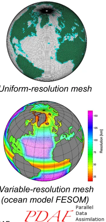
Uniform-resolution mesh
759ECHAM6–FESOM: model formulation and mean climate
2013) and uses total wavenumbers up to 63, which corre- sponds to about 1.85×1.85 degrees horizontal resolution;
the atmosphere comprises 47 levels and has its top at 0.01 hPa (approx. 80 km). ECHAM6 includes the land surface model JSBACH (Stevens et al. 2013) and a hydrological discharge model (Hagemann and Dümenil 1997).
Since with higher resolution “the simulated climate improves but changes are incremental” (Stevens et al.
2013), the T63L47 configuration appears to be a reason- able compromise between simulation quality and compu- tational efficiency. All standard settings are retained with the exception of the T63 land-sea mask, which is adjusted to allow for a better fit between the grids of the ocean and atmosphere components. The FESOM land-sea distribu- tion is regarded as ’truth’ and the (fractional) land-sea mask of ECHAM6 is adjusted accordingly. This adjustment is accomplished by a conservative remapping of the FESOM land-sea distribution to the T63 grid of ECHAM6 using an adapted routine that has primarily been used to map the land-sea mask of the MPIOM to ECHAM5 (H. Haak, per- sonal communication).
2.2 The Finite Element Sea Ice-Ocean Model (FESOM) The sea ice-ocean component in the coupled system is represented by FESOM, which allows one to simulate ocean and sea-ice dynamics on unstructured meshes with variable resolution. This makes it possible to refine areas of particular interest in a global setting and, for example, resolve narrow straits where needed. Additionally, FESOM allows for a smooth representation of coastlines and bottom topography. The basic principles of FESOM are described by Danilov et al. (2004), Wang et al. (2008), Timmermann et al. (2009) and Wang et al. (2013). FESOM has been validated in numerous studies with prescribed atmospheric forcing (see e.g., Sidorenko et al. 2011; Wang et al. 2012;
Danabasoglu et al. 2014). Although its numerics are fun- damentally different from that of regular-grid models,
previous model intercomparisons (see e.g., Sidorenko et al.
2011; Danabasoglu et al. 2014) show that FESOM is a competitive tool for studying the ocean general circulation.
The latest FESOM version, which is also used in this paper, is comprehensively described in Wang et al. (2013). In the following, we give a short model description here and men- tion those settings which are different in the coupled setup.
The surface computational grid used by FESOM is shown in Fig. 1. We use a spherical coordinate system with the poles over Greenland and the Antarctic continent to avoid convergence of meridians in the computational domain. The mesh has a nominal resolution of 150 km in the open ocean and is gradually refined to about 25 km in the northern North Atlantic and the tropics. We use iso- tropic grid refinement in the tropics since biases in tropi- cal regions are known to have a detrimental effect on the climate of the extratropics through atmospheric teleconnec- tions (see e.g., Rodwell and Jung 2008; Jung et al. 2010a), especially over the Northern Hemisphere. Grid refinement (meridional only) in the tropical belt is employed also in the regular-grid ocean components of other existing climate models (see e.g., Delworth et al. 2006; Gent et al. 2011).
The 3-dimensional mesh is formed by vertically extending the surface grid using 47 unevenly spaced z-levels and the ocean bottom is represented with shaved cells.
Although the latest version of FESOM (Wang et al.
2013) employs the K-Profile Parameterization (KPP) for vertical mixing (Large et al. 1994), we used the PP scheme by Pacanowski and Philander (1981) in this work. The rea- son is that by the time the coupled simulations were started, the performance of the KPP scheme in FESOM was not completely tested for long integrations in a global setting.
The mixing scheme may be changed to KPP in forthcom- ing simulations. The background vertical diffusion is set to 2×10⁻³m2s−1 for momentum and 10−5m2s−1 for potential temperature and salinity. The maximum value of vertical diffusivity and viscosity is limited to 0.01 m2s−1. We use the GM parameterization for the stirring due to
Fig. 1 Grids correspond- ing to (left) ECHAM6 at T63 (≈180 km) horizontal resolu- tion and (right) FESOM. The grid resolution for FESOM is indicated through color coding (in km). Dark green areas of the T63 grid correspond to areas where the land fraction exceeds 50 %; areas with a land fraction between 0 and 50 % are shown in light green
759 ECHAM6–FESOM: model formulation and mean climate
1 3
2013) and uses total wavenumbers up to 63, which corre- sponds to about 1.85×1.85 degrees horizontal resolution;
the atmosphere comprises 47 levels and has its top at 0.01 hPa (approx. 80 km). ECHAM6 includes the land surface model JSBACH (Stevens et al. 2013) and a hydrological discharge model (Hagemann and Dümenil 1997).
Since with higher resolution “the simulated climate improves but changes are incremental” (Stevens et al.
2013), the T63L47 configuration appears to be a reason- able compromise between simulation quality and compu- tational efficiency. All standard settings are retained with the exception of the T63 land-sea mask, which is adjusted to allow for a better fit between the grids of the ocean and atmosphere components. The FESOM land-sea distribu- tion is regarded as ’truth’ and the (fractional) land-sea mask of ECHAM6 is adjusted accordingly. This adjustment is accomplished by a conservative remapping of the FESOM land-sea distribution to the T63 grid of ECHAM6 using an adapted routine that has primarily been used to map the land-sea mask of the MPIOM to ECHAM5 (H. Haak, per- sonal communication).
2.2 The Finite Element Sea Ice-Ocean Model (FESOM) The sea ice-ocean component in the coupled system is represented by FESOM, which allows one to simulate ocean and sea-ice dynamics on unstructured meshes with variable resolution. This makes it possible to refine areas of particular interest in a global setting and, for example, resolve narrow straits where needed. Additionally, FESOM allows for a smooth representation of coastlines and bottom topography. The basic principles of FESOM are described by Danilov et al. (2004), Wang et al. (2008), Timmermann et al. (2009) and Wang et al. (2013). FESOM has been validated in numerous studies with prescribed atmospheric forcing (see e.g., Sidorenko et al. 2011; Wang et al. 2012;
Danabasoglu et al. 2014). Although its numerics are fun- damentally different from that of regular-grid models,
previous model intercomparisons (see e.g., Sidorenko et al.
2011; Danabasoglu et al. 2014) show that FESOM is a competitive tool for studying the ocean general circulation.
The latest FESOM version, which is also used in this paper, is comprehensively described in Wang et al. (2013). In the following, we give a short model description here and men- tion those settings which are different in the coupled setup.
The surface computational grid used by FESOM is shown in Fig. 1. We use a spherical coordinate system with the poles over Greenland and the Antarctic continent to avoid convergence of meridians in the computational domain. The mesh has a nominal resolution of 150 km in the open ocean and is gradually refined to about 25 km in the northern North Atlantic and the tropics. We use iso- tropic grid refinement in the tropics since biases in tropi- cal regions are known to have a detrimental effect on the climate of the extratropics through atmospheric teleconnec- tions (see e.g., Rodwell and Jung 2008; Jung et al. 2010a), especially over the Northern Hemisphere. Grid refinement (meridional only) in the tropical belt is employed also in the regular-grid ocean components of other existing climate models (see e.g., Delworth et al. 2006; Gent et al. 2011).
The 3-dimensional mesh is formed by vertically extending the surface grid using 47 unevenly spaced z-levels and the ocean bottom is represented with shaved cells.
Although the latest version of FESOM (Wang et al.
2013) employs the K-Profile Parameterization (KPP) for vertical mixing (Large et al. 1994), we used the PP scheme by Pacanowski and Philander (1981) in this work. The rea- son is that by the time the coupled simulations were started, the performance of the KPP scheme in FESOM was not completely tested for long integrations in a global setting.
The mixing scheme may be changed to KPP in forthcom- ing simulations. The background vertical diffusion is set to 2×10⁻³m2s−1 for momentum and 10−5m2s−1 for potential temperature and salinity. The maximum value of vertical diffusivity and viscosity is limited to 0.01 m2s−1. We use the GM parameterization for the stirring due to
Fig. 1 Grids correspond- ing to (left) ECHAM6 at T63 (≈180 km) horizontal resolu- tion and (right) FESOM. The grid resolution for FESOM is indicated through color coding (in km). Dark green areas of the T63 grid correspond to areas where the land fraction exceeds 50 %; areas with a land fraction between 0 and 50 % are shown in light green