41. Plots of cross sections and related quantities

6

41. Plots of cross sections and related quantities

σ and R in e

e

Collisions

10

-8

10

-7

10

-6

10

-5

10

-4

10

-3

10

-2

1 10 10

σ [m b ]

ω

ρ

φ

ρ

J / ψ

ψ(2S)

Υ

Z

10

-1

1 10 10

10

1 10 10

R ^ω

ρ

φ

ρ

J / ψ ψ(2S)

Υ

Z

√ s [GeV]

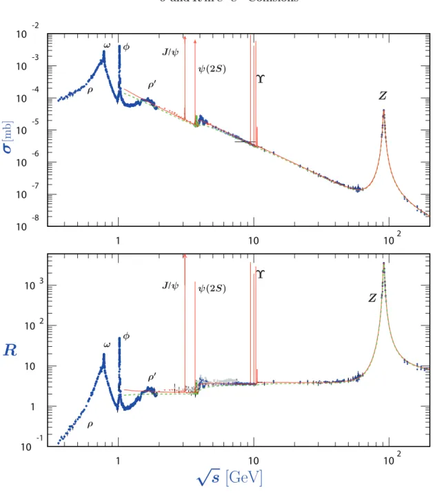
Figure 41.6: World data on the total cross section ofe⁺e⁻→hadronsand the ratioR(s) =σ(e⁺e⁻→hadrons, s)/σ(e⁺e⁻→µ⁺µ⁻, s).

σ(e⁺e⁻→hadrons, s) is the experimental cross section corrected for initial state radiation and electron-positron vertex loops,σ(e⁺e⁻→ µ⁺µ⁻, s) = 4πα²(s)/3s. Data errors are total below 2 GeV and statistical above 2 GeV. The curves are an educative guide: the broken one (green) is a naive quark-parton model prediction, and the solid one (red) is 3-loop pQCD prediction (see “Quantum Chromodynamics” section of thisReview, Eq. (9.7) or, for more details, K. G. Chetyrkinet al., Nucl. Phys.B586, 56 (2000) (Erratumibid. B634, 413 (2002)). Breit-Wigner parameterizations ofJ/ψ,ψ(2S), and Υ(nS), n= 1,2,3,4 are also shown. The full list of references to the original data and the details of theR ratio extraction from them can be found in[arXiv:hep-ph/0312114]. Corresponding computer-readable data files are available at http://pdg.lbl.gov/current/xsect/. (Courtesy of the COMPAS (Protvino) and HEPDATA (Durham) Groups, May 2010.) See full-color version on color pages at end of book.

41. Plots of cross sections and related quantities

R in Light-Flavor, Charm, and Beauty Threshold Regions

10 -1 1 10 10²

0.5 1 1.5 2 2.5 3

Sum of exclusive measurements

Inclusive measurements 3 loop pQCD Naive quark model

u, d, s

ρ ω

φ

ρ

2 3 4 5 6 7

3 3.5 4 4.5 5

Mark-I Mark-I + LGW Mark-II PLUTO DASP Crystal Ball BES

J/ψ ψ(2S)

ψ

ψ

ψ

ψ

c

2 3 4 5 6 7 8

9.5 10 10.5 11

MD-1 ARGUS CLEO CUSB DHHM

Crystal Ball CLEO II DASP LENA

Υ(1S)

Υ(2S) Υ(3S)

Υ(4S)

b

R

√ s [GeV]

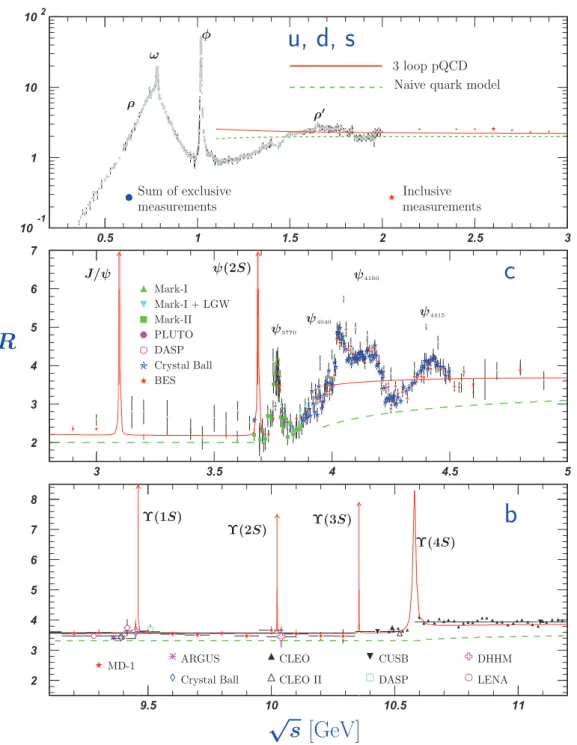
Figure 41.7: Rin the light-flavor, charm, and beauty threshold regions. Data errors are total below 2 GeV and statistical above 2 GeV.

The curves are the same as in Fig. 41.6.Note:CLEO data above Υ(4S) were not fully corrected for radiative effects, and we retain them on the plot only for illustrative purposes with a normalization factor of 0.8. The full list of references to the original data and the details of theR ratio extraction from them can be found in[arXiv:hep-ph/0312114]. The computer-readable data are available at http://pdg.lbl.gov/current/xsect/. (Courtesy of the COMPAS (Protvino) and HEPDATA (Durham) Groups, May 2010.) See full-color version on color pages at end of book.