Knowledge----Based Protein Loop Prediction and Based Protein Loop Prediction and Based Protein Loop Prediction and Based Protein Loop Prediction and Ab

(1)

Protein Protein Protein

Protein Structure Structure Structure and Enzyme Catalysis: Structure and Enzyme Catalysis: and Enzyme Catalysis: and Enzyme Catalysis:

Knowledge Knowledge Knowledge

Knowledge----Based Protein Loop Prediction and Based Protein Loop Prediction and Based Protein Loop Prediction and Based Protein Loop Prediction and Ab

Ab Ab

Ab Initio Initio Initio Initio Equilibrium Constant Estimation Equilibrium Constant Estimation Equilibrium Constant Estimation Equilibrium Constant Estimation

Inaugural-Dissertation zur

Erlangung des Doktorgrades

der Mathematisch-Naturwissenschaftlichen Fakultät der Universität zu Köln

vorgelegt von Quoc-Vu Ha Ngoc

aus Bonn

Köln, April 2008

(2)

1. Berichterstatter: Universitätsprofessor Prof. Dr. D. Schomburg 2. Berichterstatter: Universitätsprofessor Prof. Dr. H. W. Klein

Tag der mündlichen Prüfung: 25. April 2008

(3)

Danksagung Danksagung Danksagung Danksagung

Prof. Dr. Dietmar Schomburg danke ich besonders für die Möglichkeit diese Dissertation durchführen zu können. Seine kompetente und herzliche Betreuung waren für mich eine große Bereicherung. Für seine Unterstützung und sein Vertrauen über die Jahre möchte ich mich herzlich bedanken.

Sehr herzlich möchte ich auch Prof. Dr. Helmut W. Klein für die freundliche Übernahme des Zweitgutachtens danken.

Dr. Gerd Wohlfahrt danke ich für die angenehme und erfolgreiche Zusammenarbeit bei der Loopvorhersage.

Mein Dank gilt auch Dr. Kai Hartmann in dem ich neben einem zuverlässigen stets hilfsbereiten Kollegen auch einen guten Freund gefunden habe, der mir bei der Vorhersage der Gleichgewichtskonstanten mit Rat und Sachverstand zur Seite stand.

Bedanken möchte ich mich auch bei Dr. Lars Packschies für die persönliche Betreuung bei der Bedienung der quantenmechanischen Software. Seine Hilfsbereitschaft, seine anregenden Ideen und sein Engagement haben wesentlich zum Gelingen dieses Projektes beigetragen.

Besonders bedanke ich mich bei meinen Eltern für ihre Geduld, ihre beständige Unterstützung, und dass sie stets für mich da waren.

(4)

Abstract Abstract Abstract Abstract

Prediction methods in the field of bioinformatics can be divided into

ab initio

and knowledge-based methods. The work in this thesis investigates the importance of anchor group positioning in knowledge-based protein loop prediction as well as the

ab initio

estimation of equilibrium constants using Density Functional Theory (DFT).

The maximum possible prediction quality of knowledge-based loop prediction was examined for 595 insertions and 589 deletions with respect to gap length, fragment length, amino acid type, secondary structure and relative solvent accessibility while applying all possible anchor group positions for the fitting of loops between 3 and 12 residues in length.

It was possible to predict 74.3 % of insertions and 83.7 % of deletions within an RMS deviation of < 1.5 Å between template and target structure using a knowledge-based fragment databank based on structures of the Protein Databank (PDB). The analysis showed that the importance of anchor group positioning increases with gap length and that medium fragments with lengths between 5-8 residues perform better than shorter or longer fragments. In addition, better predictions were obtained when anchor groups consisted of hydrophobic residues, were located within secondary structures such as helices and beta sheets, or had low relative solvent accessibilities. A test based on targeted anchor group selection using a combination of the above criteria showed an improvement in prediction quality compared to a random selection of anchor groups.

Density Functional Theory (DFT) with a b3lyp/6-311g++ (d,p) basis set was used in combination with a preceding molecular mechanics conformational search to estimate the standard transformed Gibbs free energies of reaction (∆G^r°’) for a set of 45 enzyme-catalyzed reactions at standard biochemical conditions (pH 7 and 298.15 K). For reactions from EC group 1 and EC groups 5 and 6, the calculated ∆G^r°’ values deviated from the experimental

(5)

values by an average of 2.49 kcal/mol and 5.50 kcal/mol, respectively. This data was comparable to the values calculated using group contribution method by Mavrovouniotis (Mavrovouniotis, J.Biol.Chem 1991; 266:14440-45), where the mean error was 2.76 kcal/mol for reactions from EC group 1 and 4.76 kcal/mol for reactions from EC groups 5 and 6. The mean error for the entire set of reactions was 10.30 kcal/mol. These results are very promising, considering that purely structural information was used, and the method can be improved by further optimization.

(6)

Zu Zu Zu

Zusammenfassung sammenfassung sammenfassung sammenfassung

Vorhersagemethoden auf dem Gebiet der Bioinformatik lassen sich unterscheiden zwischen

ab initio

und wissensbasierten Methoden. In dieser Dissertation wird sowohl der Einfluss der Ankergruppenpositionierung auf die Qualität der wissensbasierten Loopvorhersage untersucht, sowie eine

ab initio

Abschätzung von Gleichgewichtskonstanten mithilfe der Dichte Funktional Theorie (DFT) vorgenommen.

Für die wissensbasierte Loopvorhersage von 595 Insertionen und 589 Deletionen wurde die maximal mögliche Vorhersagequalität in Abhängigkeit von Gaplänge, Fragmentgröße, Aminosäuretyp, Sekundärstruktur und relativer Lösungsmittel- zugänglichkeit ermittelt. Dabei wurden alle Ankergruppenpositionen berücksichtigt, die bei einer Modellierung von Loops zwischen 3 und 12 Aminosäureresten möglich waren.

74.3 % der Insertionen und 83.7 % der Deletionen könnten mit einer RMS Abweichung von unter 1.5 Å zwischen Leit- und Zielstruktur anhand einer PDB-Struktur basierten Fragmentdatenbank vorausgesagt werden. Die Untersuchungen ergaben, dass der Einfluss der Ankergruppenpositionierung mit Länge der Gaps zunimmt, und dass mittellange Fragmente zwischen 5 und 8 Aminosäurereste bessere Vorhersageergebnisse erzielen, als kurze oder lange Fragmente. Ausserdem wurden bessere Vorhersagen erreicht, wenn die Ankergruppen entweder aus hydrophoben Aminosäureresten bestanden, innerhalb von Sekundärstrukturen wie Helices oder Beta-Faltblätter lagen, oder eine niedrige Lösungsmittelzugänglichkeit besaßen. In einem Test wurden die Ankergruppen durch Kombination der oben genannten Kriterien gezielt ausgewählt, wodurch, im Vergleich zur zufälligen Ankergruppenwahl, eine deutliche Verbesserung der maximalen Vorhersagequalität erzielt wurde.

(7)

Für 45 Enzymreaktionen unter Standardbedingungen (pH 7 und 298.15K) wurden die freien Reaktionsenthalpien (∆G^r°’) über quantenmechanische Berechnung der freien Enthalpien der Metabolite bestimmt, und die Vorhersagequalität durch Vergleich mit den experimentell ermittelten Gleichgewichtskonstanten untersucht. Die Berechnung der freien Enthalpien der Metabolite erfolgte nach molekularmechanischer Konformations- minimierung unter Anwendung der Dichte Funktional Theorie (DFT) mit dem b3lyp/6-311g++ (d,p) Basissatz. Die berechneten freien Reaktionsenthalpien unterschieden sich im Durchschnitt von den experimentellen Werten um 2.49 kcal/mol bei Reaktionen der EC Gruppe 1, und um 5.50 kcal/mol bei Reaktionen der EC Gruppen 5 und 6. Diese Werte waren vergleichbar mit denen, die durch Anwendung der Inkrementmethode von Mavrovouniotis (Mavrovouniotis, J.Biol.Chem 1991; 266:14440-45) erzielt wurden. Dort lag der Durchschnittsfehler bei 2.76 kcal/mol für Reaktionen der EC Gruppe 1, und 4.76 kcal/mol für Reaktionen der EC Gruppen 5 und 6. Für den gesamten Satz der Reaktionen betrug der Vorhersagefehler im Durchschnitt 10.30 kcal/mol. Diese Resultate können als sehr vielversprechend gewertet werden, da ausschliesslich reine Strukturinformationen verwandt wurden, und sie können durch weitere Optimierung der Methode noch verbessert werden.

(8)

List of List of List of

List of Abbreviations Abbreviations Abbreviations Abbreviations and Constants and Constants and Constants and Constants

∆G°’^tot - Total standard transformed Gibbs free energy (298.15K, I=0, 1M, pH7)

∆G°^tot - Total standard Gibbs free energy (298.15K, I=0, 1M)

∆G^f° - Standard Gibbs free energy of formation (298.15K, I=0, 1M)

∆G^f°’ - Standard transformed Gibbs free energy of formation (298.15K, I=0, 1M, pH7)

∆G^r° - Standard Gibbs free energy of reaction (298.15K, I=0, 1M)

∆G^r°’ - Standard transformed Gibbs free energy of reaction (298.15K, I=0, 1M, pH7) a.u. - Atomic units (1 a.u. = 1 Hartree = 2625.5 kJ/mol)

COSMO - Conductor-like Screening Model DFT - Density Functional Theory

EC - Enzyme Commission

FSSP - Families of Structurally Similar Proteins I - Ionic Strength (mol/l)

K - Equilibrium Constant

K’ - Apparent Equilibrium Constant

kcal and kJ - Kilocalories and Kilojoules (1 kcal = 4.184 kJ) MMFF - Merck Molecular Force Field

NBS - National Bureau of Standards

NIST - National Institute of Standards and Technology PDB - Protein Databank

PM3 - Parametrized Model Number 3 R - Gas Constant (R= 8.314472 J K^-1 mol^-1) SCOP - Structural Classification of Proteins

(9)

List of Figures List of Figures List of Figures List of Figures

Figure 2.1: The 20 Naturally Occurring Proteinogenic Amino Acids... 7

Figure 2.2: Peptide Bond Formation. ... 8

Figure 2.3: Venn Diagram of Amino Acid Properties. ... 10

Figure 2.4: Ramachandran Plot. ... 12

Figure 2.5: Right-Handed α-Helix and Parallel/Anti-Parallel β-Sheet. ... 14

Figure 2.6: Supersecondary Structure Elements. ... 17

Figure 2.7: Energy Landscape of Protein Folding... 21

Figure 2.8: CATH Protein Classification System. ... 25

Figure 2.9: Decomposition of Glutamate at pH 7 into Functional Groups. ... 52

Figure 2.10: Effect of Polarization Functions on Neighboring Orbitals... 60

Figure 2.11: Solvent Accessible Surface. ... 63

Figure 4.1: Maximum Prediction Quality. ... 86

Figure 4.2: Maximum Prediction Quality sorted by Gap Length. ... 88

Figure 4.3: Influence of Loop Fragment Length. ... 90

Figure 4.4: Influence of Amino Acid Type. ... 92

Figure 4.5: Influence of Secondary Structure. ... 94

Figure 4.6: Influence of Relative Solvent Accessibility... 96

Figure 4.7: Prediction using Combination of Criteria. ... 97

Figure 4.8: Prediction using Combined Odds Ratios vs. Random Anchor Groups. ... 98

Figure 4.9: Mean Absolute Error for Estimation of ∆G r°’. ... 103

(10)

List of T List of T List of T

List of Tables ables ables ables

Table 2.1: Frequency of Occurrence of Amino Acids... 10

Table 2.2: Parameters for Common Regular Polypeptide Conformations... 13

Table 2.3: Protein Data Bank (PDB) Statistics of February 2008. ... 32

Table 2.4: Top Level EC Numbers (EC Groups). ... 35

Table 2.5: Calculation of ∆G^r°’ of Glutamate using Group Contributions. ... 52

Table 2.6: Nomenclature for Split-Valence Basis Sets by Pople... 58

Table 3.1: Fragment Databank Based on all Structures from PDB 2/98. ... 70

Table 3.2: Test Data Set of Loops with all Possible Anchor Group Positions... 72

Table 3.3: Input Commands for

Gaussian 03

... 79

Table 4.1: Maximum Prediction Quality for Test Data Set. ... 86

Table 4.2: Maximum Prediction Quality sorted by Gap Length. ... 87

Table 4.3: Prediction Quality sorted by Length of Loop Fragments... 89

Table 4.4: Prediction Quality sorted by Individual Amino Acids... 91

Table 4.5: Prediction Quality sorted by Amino Acid Type. ... 92

Table 4.6: Prediction Quality sorted by Secondary Structure Combination. ... 93

Table 4.7: Prediction Quality sorted by Relative Solvent Accessibility... 95

Table 4.8: Prediction using Combination of Criteria. ... 98

Table 4.9: Effect of Conformational Search on Gibbs Free Energy of Reaction (∆G^r°’). 99 Table 4.10: Effect of Solvation Model on Gibbs Free Energy of Reaction (∆G^r°’)... 100

Table 4.11: Standard Transformed Gibbs Free Energies of Reaction (∆G^r°’). ... 101

Table 6.1: Standard Servers and Software Packages used in this Project... 119

Table 6.2: List of Reactions for Estimation of Reaction Equilibrium using DFT. ... 120

Table 6.3: Total Standard Gibbs Free Energies of Metabolites determined by DFT. ... 122

(11)

Table of Contents Table of Contents Table of Contents Table of Contents

1111 INTRODUCTIONINTRODUCTION ...INTRODUCTIONINTRODUCTION... 1111...

1.1 Purpose and Motivation ... 1

1.2 Specific Aims... 3

1.2.1 Anchor Group Positioning in Knowledge-Based Loop Prediction 3 1.2.2

Ab Initio

Equilibrium Constant Estimation using DFT... 4

2222 BACKGROUNDBACKGROUND ...BACKGROUNDBACKGROUND... 5555...

2.1 Protein Structure ... 5

2.1.1 Introduction ... 5

2.1.2 Amino Acids and Primary Structure ... 6

2.1.3 Secondary Structure... 11

2.1.4 Supersecondary Structure... 16

2.1.5 Tertiary Structure and Folding ... 18

2.1.6 Homology... 22

2.1.7 Structure Classification... 24

2.1.8 Structure Determination Methods... 26

2.1.9 Protein Data Bank (PDB) ... 31

2.1.10 Enzymes ... 33

2.2 Protein Structure Prediction... 36

2.2.2

Ab Initio

Modeling ... 37

2.2.3 Fold Recognition Modeling... 38

2.2.4 Homology Modeling... 38

2.2.5 Loop Prediction... 40

2.3 Chemical Equilibrium ... 43

2.3.2 Equilibrium Constant (K) ... 44

2.3.3 Temperature Dependence of Equilibrium Constants ... 47

2.3.4 Apparent Equilibrium Constant (K’) ... 47

2.3.5 Standard State Convention in Biochemical Reactions... 48

2.3.6 Group Contribution Method... 50

2.4

Ab Initio

Computational Quantum Mechanics ... 53

(12)

2.4.2 Schrödinger Equation and Born-Oppenheimer Approximation.. 54

2.4.3 Basis Functions... 56

2.4.4 Basis Sets... 57

2.4.5 Quantum Mechanical Calculations... 60

2.4.6 Solvation Models... 62

2.4.7 Quantum Mechanical Methods ... 64

3333 MATERIAMATERIALS AND METHODSMATERIAMATERIALS AND METHODSLS AND METHODSLS AND METHODS...69...696969 3.1 Anchor Group Positioning in Knowledge-Based Loop Prediction... 69

3.1.1 Fragment Data Bank ... 69

3.1.2 Test Data Set of Aligned Protein Pairs ... 70

3.1.3 Anchor Group Positioning ... 71

3.1.4 Loop Modeling and Ranking... 72

3.1.5 Data Evaluation and Correlation to Anchor Groups ... 73

3.2

Ab Initio

3.2.1 Retrieval of Reactions from NIST Enzyme Database... 74

3.2.2 Database Format Conversion and Data Processing... 75

3.2.3 Calculation of Reaction Equilibrium using Group Contributions 76 3.2.4 Conformational Space Search using

Spartan 06

... 76

3.2.5 Estimation of pKa using

MarvinSketch

... 77

3.2.6 Quantum Mechanical Calculations using

Gaussian 03

... 78

3.2.7 Determination of Gibbs Free Energies of Metabolites (∆G°’^tot).... 79

3.2.8 Calculation of Gibbs Free Energies of Reaction (∆G^r°’)... 83

4444 RESULTSRESULTS ...RESULTSRESULTS...85858585 4.1 Anchor Group Positioning in Knowledge-Based Loop Prediction... 85

4.1.1 Maximum Prediction Quality ... 85

4.1.2 Influence of Loop Fragment Length ... 88

4.1.3 Influence of Amino Acid Type ... 90

4.1.4 Influence of Secondary Structure ... 93

4.1.5 Influence of Solvent Accessibility... 95

4.1.6 Prediction using Combination of Criteria ... 96

4.2

Ab Initio

4.2.1 Effect of Conformational Search Method... 99

4.2.2 Effect of Solvation Model ... 100

4.2.3 Standard Transformed Gibbs Free Energy of Reaction (∆G^r°’) .. 101

(13)

5555 DISCUSSIONDISCUSSION...DISCUSSIONDISCUSSION...104104104104

5.1 Anchor Group Positioning in Knowledge-Based Loop Prediction... 104

5.1.1 Interpretation of Results... 104

5.1.2 Outlook... 106

5.2

Ab Initio

5.2.1 Interpretation of Results... 107

5.2.2 Outlook... 109

6666 APPENDIXAPPENDIX...APPENDIXAPPENDIX...111111111111 6.1 Databases ... 111

6.1.1 Protein Databank (PDB)... 111

6.1.2 NIST Database of Enzyme Reactions... 112

6.1.3 BRENDA (BRaunschweig ENzyme DAtabase) ... 112

6.1.4 KEGG (Kyoto Encyclopedia of Genes and Genomes)... 113

6.2 Software Packages... 114

6.2.1

Gaussian 03

... 114

6.2.2

Spartan ‘06

... 115

6.2.3

Gibbspredictor

... 115

6.2.4

JChem

... 116

6.2.5

NIST2MySQL

... 116

6.2.6

GaussView

... 117

6.2.7 Database Management Software ... 117

6.3 Hardware and Computer Resources ... 119

6.3.1 Servers ... 119

6.3.2 Local Workstation ... 119

6.4 List of Reactions... 120

6.5 List of Metabolites... 122 7777 REFEREFERENCESREFEREFERENCESRENCESRENCES...126126126126

(14)

CHAPTER 1 CHAPTER 1 CHAPTER 1 CHAPTER 1

1111 INTRODUCTION INTRODUCTION INTRODUCTION INTRODUCTION

1.1 1.1 1.1

1.1 Purpose and Motivation Purpose and Motivation Purpose and Motivation Purpose and Motivation

Prediction methods in the field of bioinformatics can be divided into

ab initio

and knowledge-based methods. This thesis investigates the importance of anchor group positioning in knowledge-based protein loop prediction as well as the

ab initio

estimation of equilibrium constants using Density Functional Theory (DFT).

The prediction of protein loops around insertions and deletions represents one of the major challenges in protein structure prediction. In knowledge-based structure prediction, loop modeling creates the second largest source of error next to template-target alignment.

The quality of loop prediction is dependent upon several factors such as the algorithm for fragment selection, the completeness of the fragment databank, the fitting/optimization procedure, and the choice of anchor groups. The present thesis will investigate the effect of anchor group selection on loop prediction quality with respect to a variety of criteria including gap length, fragment length, amino acid type, secondary structure, and relative solvent accessibility. Finally, a combination of the criteria will be used for selecting optimal

(15)

anchor groups for a loop prediction scenario, and the prediction quality compared to a dataset with randomly chosen anchor groups.

Biochemical reactions are catalyzed by highly specific enzymes which, by lowering the activation energy, allow reactions to run at highly increased rates. However, the feasibility and direction of a biochemical reaction are determined by its equilibrium. Since equilibrium constants are usually not available for any random biochemical reaction without major experimental efforts, methods have been developed to predict them independently from experimental measurements. One such method is the group contribution method by Mavrovouniotis [68][69]. The method is, however, limited to reactions at standard biochemical conditions (pH 7 and 298.15K) and biased towards the biochemical metabolites from which the set of contributions were derived. It has therefore been desirable to find a methods such as, for example, a

b initio

molecular quantum mechanical calculations which work independently from any experimental data. However in the past, the

ab initio

approach has always been problematic, as computers and theories were not sufficiently developed to generate energy data in a manageable time frame and with acceptable accuracy. Density Functional Theory (DFT) method [58] has, so far, offered the best compromise between accurate results and acceptable calculation times. The COSMO solvation model [57] has also shown to deliver fast and accurate calculations with respect to solvation energies. This project aims at using the recent developments in hardware, software, and quantum mechanical methods in an attempt to develop a procedure for estimating experimental biochemical equilibrium constants in a timely manner and independently from empirical data. The standard transformed Gibbs free energies of reactions (∆G^r°’) will be determined from the total standard Gibbs free energies (∆G°^tot) of the metabolites, which were calculated by using Density Functional Theory (DFT). The calculated values will then be compared with experimental equilibrium constants provided by the National Institute of Standards and Technology (NIST) Database of Enzyme Reactions.

(16)

1.2 1.2

1.2 1.2 Specific Specific Aims Specific Specific Aims Aims Aims

1.2.1 1.2.1 1.2.1

1.2.1 Anchor Group Anchor Group Anchor Group Anchor Group Positioning in Knowledge Positioning in Knowledge Positioning in Knowledge----Based Loop Prediction Positioning in Knowledge Based Loop Prediction Based Loop Prediction Based Loop Prediction

Specific Aim 1:

Specific Aim 1: Creation of a test dataset of insertions and deletions by 3-D alignment of protein pairs followed by identification of all possible anchor groups for each insertion/deletion.

Specific Aim Specific Aim Specific Aim

Specific Aim 2: 2: 2: 2: Fitting of loop fragments using a fragment databank made from experimental structures of the Protein Databank (PDB) [43] followed by determination of global RMS deviation between template and target and identification of the best fitting fragment for each anchor group combination.

Specific Aim 3:

Specific Aim 3: Evaluation of maximum prediction quality dependent on gap length, fragment length, and anchor group properties such as amino acid type, secondary structure, and relative solvent accessibility, followed by a test using a combination of the above criteria for determining optimal anchor groups.

(17)

1.2.2 1.2.2 1.2.2

1.2.2 Ab Ab Ab Ab IIIInitio nitio nitio nitio Equilibrium Constant E Equilibrium Constant Estimation using DFT Equilibrium Constant E Equilibrium Constant E stimation using DFT stimation using DFT stimation using DFT

Specific Aim 1:

Specific Aim 1: Retrieval of biochemical reactions, reaction conditions, and equilibrium constants from the NIST Database of Enzyme Reactions [22], followed by the creation of a database containing only data from reactions at standard biochemical conditions (298.15 K and pH 7).

Specific Aim 2:

Specific Aim 2: Identification of the appropriate percentage distribution for the charge isomers of each metabolite at pH 7 by using the pka prediction tool

MarvinSketch

[36], followed by a global conformational search using

Spartan 06

[47], followed by energy minimization and total standard Gibbs free energy (∆G°^tot) calculation using

Gaussian 03

[39].

Specific Aim 3:

Specific Aim 3: Evaluation of the transformed standard Gibbs free energies of reaction (∆G^r°’) by subtracting the total standard Gibbs free energies (∆G°^tot) of products minus reactants in each reaction, followed by an error estimation between values calculated by DFT [58] and experimental values obtained from the NIST Database of Enzyme Reactions [22].

(18)

2222 BACKGROUND BACKGROUND BACKGROUND BACKGROUND

2.1 2.1

2.1 2.1 Protein Structure Protein Structure Protein Structure Protein Structure

2.1.1 2.1.1 2.1.1

2.1.1 Introduction Introduction Introduction Introduction

Proteins play a role in almost all processes within a living organism. They are involved in the duplication and expression of genetic material, they take part in signal transduction and storage of particles, and they arrange into structural elements such as muscle, bone, tendons, hair, and nails. As antibodies, proteins constitute a major part of the immune system, and as enzymes they allow the progression of life-sustaining chemical reactions at acceptable rates under physiologic conditions.

The functional diversity of proteins is rooted in their structure. Proteins basically consist of one or more unbranched chains of amino acids which fold into a three- dimensional topology. The enormous variety of three-dimensional structures can be attributed to the chemical diversity of the twenty proteinogenic amino acids (Figure 2.1) as well as the possible number of sequences by which they can be arranged. Knowledge about the exact structure of proteins plays a key role in understanding their function. Proteins basically operate by binding specifically and tightly to other molecules.

(19)

The structure of proteins can be organized into hierarchical levels also referred to as primary, secondary, tertiary, and quarternary structure. The primary structure of a protein is defined by its sequence of amino acids, while the secondary structure describes local regular conformations of the backbone. Tertiary structure represents the three-dimensional shape of a protein and quarternary structure characterizes the aggregation of several polypeptide strands into multi-domain complexes. The primary sequence of amino acids contains all the information necessary for generating a stable three-dimensional protein structure [3].

2.1.2 2.1.2 2.1.2

2.1.2 Amino Acids and Primary Structure Amino Acids and Primary Structure Amino Acids and Primary Structure Amino Acids and Primary Structure

Proteins are polymers made of linear chains of amino acids. A protein can consist anywhere from 50 to 25000 amino acid residues, with most proteins averaging between 200 to 300 residues [91]. Amino acids consist of an amino and a carboxyl group bonded to a central carbon atom also referred to as the C^α atom. The C^α atom also carries one of 20 different amino acid side chains and can be found in the L-configuration in almost all proteins. The relative frequency in which each amino acid is found in a polypeptide chain is rather constant across natural proteins (Table 2.1). Some variations are found in membrane proteins, where the fraction of hydrophobic residues is increased, or in special proteins such as collagen which contains repetitive patterns of glycine and proline residues [19].

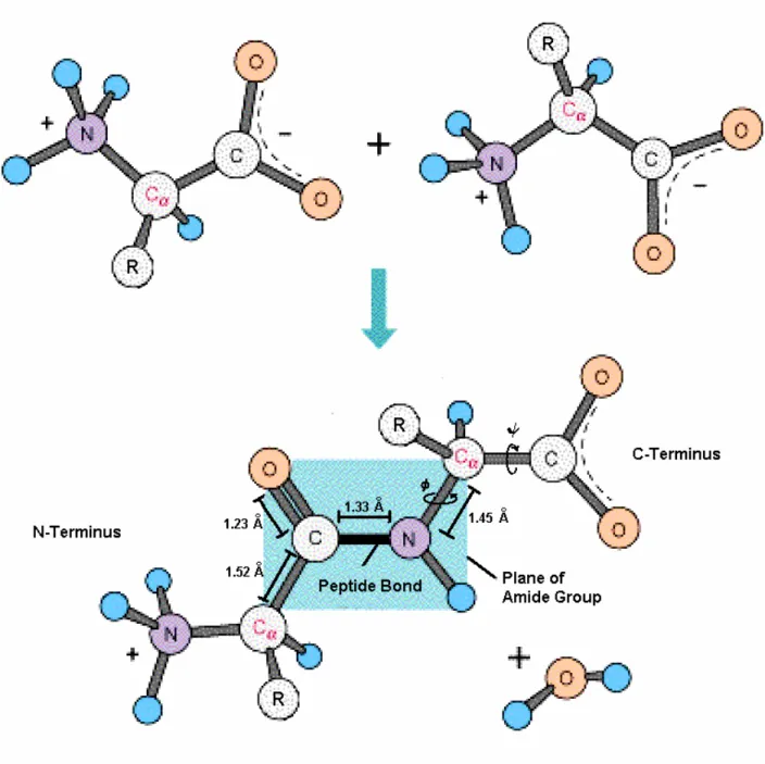
Polypeptide chains are formed by condensation of the carboxyl and amino groups of successive amino acid residues, thus creating the protein backbone (Figure 2.2). Due to resonance, the peptide bond exerts about 40% double bonded character, so that the six surrounding atoms have a coplanar geometry in which neighboring C^α atoms are mostly found in the sterically favored

trans

(180°) conformation [85]. Rotations within the backbone are restricted to the two backbone torsion angles (φ and ψ) around the C^α atom (Figure 2.2).

(20)

Figure Figure Figure

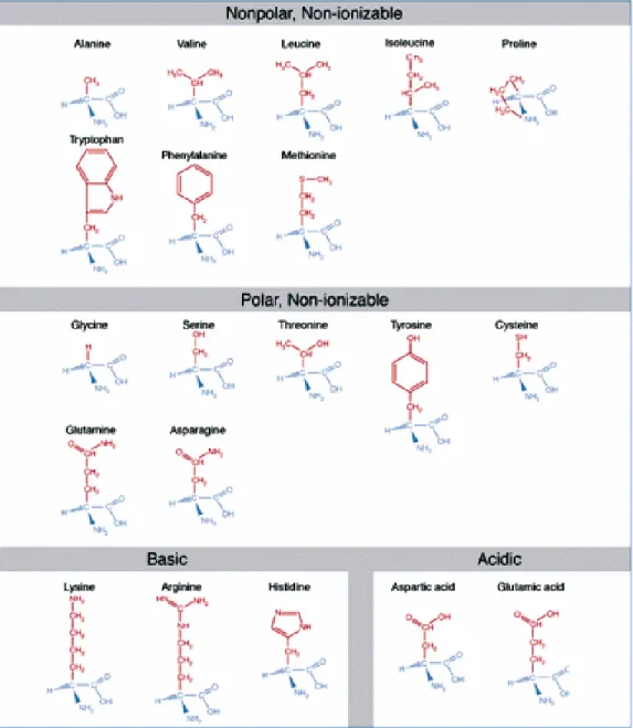
Figure 2222....1111:::: The 20 The 20 The 20 The 20 Naturally ONaturally ONaturally ONaturally Occurriccurriccurring Pccurring Png Proteinogenic ng Proteinogenic roteinogenic roteinogenic AAAAmino mino mino Amino AAAcidscidscidscids. . . . Amino acids are grouped by chemical properties of their side chains. Except for the non-chiral glycine, amino acids are found in the L-configuration in almost all proteins.

___________________________________________________________________

source: http://trc.ucdavis.edu/biosci10v/bis10v/week2/2webimages/ch5-amino-acids.jpg

(21)

Figure 2222....2222:::: Peptide Bond Formation.Peptide Bond Formation.Peptide Bond Formation.Peptide Bond Formation. Two amino acids are joined by condensation of adjacent amino and carboxyl groups. The peptide bond has a length of 1.33 Å which lies between the average C-N single bond (1.45 Å) and C=N double bond (1.25 Å) [84].

Planar configuration restricts backbone rotation to the two torsion angles φ and ψ.

___________________________________________

source: http://hykim.cbnu.ac.kr/lectures/cellbio/3/3.htm

(22)

Amino acids differ in their structure and chemical properties. While most amino acids can be classified by general chemical characteristics such as size, charge, and polarity (Figure 2.3), some residues possess additional unique features. Glycine, for example, has no side chain and is therefore a sterically highly flexible residue. Cysteine is special in that two residues can create disulfide bridges by oxidation. Proline is an imino acid and the only residue that can form stable peptide bonds in

cis

-conformation. Proline can often be found in loops and turns (Chapt. 2.1.3).

The primary sequence of a protein can be analyzed by chemical methods. The amino acid composition is routinely identified by the complete hydrolysis of all backbone peptide bonds using 6 M HCL at about 110°C for 24-72 hours followed by chromatographic analysis of the released amino acids [27]. The most successful chemical method for determining the exact protein primary sequence has been a procedure known as Edman Degradation [14].

This procedure identifies the amino acid sequence beginning from the N-terminal residue of a polypeptide. The free N-terminus reacts with phenylisothiocyanate in basic medium followed by cleavage of the residue with trifluoroacetic acid to give the phenylthiocarbamyl (PTC) peptide. The released PTC peptide rearranges in aqueous solution to the phenylthiohydantoin (PTH) derivative and can be analyzed by chromatographic methods.

By repeatedly subjecting the remaining shortened polypeptide to this procedure, one eventually obtains the entire amino acid sequence. As of today, more than 5.1 million protein sequences have been determined and are currently stored in the UniProt/TrEMBL databank [38].

(23)

Figure 2222....3333:::: Venn Diagram Venn Diagram Venn Diagram Venn Diagram of Amino Acid Propof Amino Acid Propof Amino Acid Propertiesof Amino Acid Propertiesertieserties.

______________________________________________

__________________________________________________________________________________________ ____________

source: http://www.dreamingintechnicolor.com/InfoAndIdeas/AminoAcids.gif

Table Table Table

Table 2222....1111:::: Frequency of Occurrence of Amino AFrequency of Occurrence of Amino AFrequency of Occurrence of Amino AFrequency of Occurrence of Amino Acids.cids.cids. cids.

Amino Acid Residue Mass (Daltons) Frequency in Proteins (%)^*

Ala (A) 71.09 8.3

Arg (R) 156.19 5.7

Asn (N) 114.11 4.4

Asp (D) 115.09 5.3

Cys (C) 103.15 1.7

Gln (Q) 128.14 4.0

Glu (E) 129.12 6.2

Gly (G) 57.05 7.2

His (H) 137.14 2.2

Ile (I) 113.16 5.2

Leu (L) 113.16 9.0

Lys (K) 128.17 5.7

Met (M) 131.19 2.4

Phe (F) 147.18 3.9

Pro (P) 97.12 5.1

Ser (S) 87.08 6.9

Thr (T) 101.11 5.8

Trp (W) 186.21 1.3

Tyr (Y) 163.18 3.2

Val (V) 99.14 6.6

*Frequency was determined across 1021 unrelated proteins of known sequence. _____________________________________________

source: P. McCaldon and P. Argos, Proteins 4:99-122, 1988

(24)

2.1.3 2.1.3 2.1.3

2.1.3 Secondary Structure Secondary Structure Secondary Structure Secondary Structure

The structure of a protein is primarily determined by its backbone conformation. Due to the partially double bonded character of the peptide bond, the protein backbone can be considered a chain of successive coplanar peptide units which are joined together at the C^α atoms and rotate around the two torsion angles φ and ψ (Chapt. 2.1.2). Since these two angles of rotation represent the only degrees of freedom for the protein main chain, its conformation can be completely characterized when the torsion angles φ and ψ for all residues are known. Steric collisions between side chain and backbone atoms lead to a restriction in the number of allowed conformational angles for φ and ψ. The permitted values of φ and ψ were first determined by Ramachandran using hard-sphere models with fixed bond lengths and recorded on a two-dimensional map known as the Ramachandran plot [86]. The authors observed that the flexibility of alanine residues was quite limited, with fully allowed regions occupying about 7.5% and partially allowed regions occupying about 22.5% of the total plot area (Figure 2.4). Plots for the other amino acids look similar with the exception of glycine which has more rotational freedom due to its lack of a chiral side chain.

The allowed regions of the Ramachandran plots contain specific torsion angle combinations which are repetitively found along stretches within natural proteins and are also referred to as regular conformation or secondary structure. Regular conformations are primarily stabilized by hydrogen bonding among polar atoms of the protein backbone. In a secondary structure, all amino acid residues have close to identical torsion angles and create a helical pattern characterized by a fixed number of residues per turn and translation distance per residue. Parameters of some common secondary structures are listed in Table 2.2, and their torsion angles are also found within the fully regions of the Ramachandran plot (Figure 2.4).

(25)

Figure 2222....4444:::: Ramachandran PloRamachandran PloRamachandran PloRamachandran Plotttt. Permitted values of φ and ψ torsion angles determined using a model of alanine with hard-sphere atoms and fixed bond geometries. Fully allowed regions are dark-shaded while partially allowed regions are light-shaded. Regular conformations are marked and include anti-parallel β-sheet (1)(1)(1), polyproline I/II and (1) polyglycine (2)(2)(2)(2), parallel β-sheet (3)(3)(3), 3(3) ¹⁰-helix (4)(4)(4)(4), right-handed α-helix (5)(5)(5), π-helix (5) (6)

(6) (6)

(6), and left-handed α-helix (7)(7)(7) [86]. (7) ______________________________________________

______________________________________________

_______________________________________________________________ ___

source: http://fmc.unizar.es/people/fff/Jsancho1/ramachandran.jpg

The most commonly observed secondary structure in natural proteins is the right- handed α-helix. In globular proteins, 31% of residues are located in α-helices [50]. The right- handed α-helix has 3.6 residues per turn, a translation of 1.50 Å per residue, and torsion angles of φ = -57° and ψ = -47° (Table 2.2). Most α-helices are between 10-15 residues in length and they are stabilized through hydrogen bonding of the backbone between the C=O

(26)

of the i^th residue and the -NH of the i+4^th residue further down the chain (Figure 2.5 B). The dipole moment of the hydrogen bonds is pointed parallel and in the direction of the dipole moment of the peptide groups so that they complement each other. The entire α-helix can thus be seen as a macrodipole with a negatively charged carboxyl end and positively charged amino end (Figure 2.5 A), with the absolute value of the helix dipole moment being proportional to the number of residues. The side chains of the α-helix residues point outward the helical cylinder with some α-helices having primarily non-polar residues located along one side and polar residues along the opposite side. These α-helices are also known as amphiphatic helices (Figure 2.5 C&D) and they tend to aggregate into larger structures like helix bundles or coiled coils (Chapt. 2.1.4). Other known helices include the 3¹⁰ helix, the left-handed α-helix, and the π-helix. The 3¹⁰ helix can be found at the finishing stretches of right-handed α-helices, while the other two helix types are almost never observed in natural proteins. Features of the polyproline and polyglycine helices can be found as part of the collagen triple helix [77].

Table Table Table

Table 2222....2222:::: Parameters for Common RegulParameters for Common RegulParameters for Common RegulParameters for Common Regular Polypeptide Conformationsar Polypeptide Conformationsar Polypeptide Conformations ar Polypeptide Conformations

Regular Conformation Bond Angle (degrees) Residues Translation Φ ψ ω per Turn per Residue (Å) Anti-parallel β-sheet -139 +135 -178 2.0 3.4 Parallel β-sheet -119 +113 180 2.0 3.2 Right-handed α-helix - 57 - 47 180 3.6 1.5 310 –helix - 49 - 26 180 3.0 2.0 π – helix - 57 - 70 180 4.4 1.15 Polyproline I (right-handed) - 83 +158 0 3.33 1.9 Polyproline II (left-handed) - 78 +149 180 3.0 3.1 Polyglycine - 80 +150 180 3.0 3.1 _____________________________________________________________

source: Ramachandran and Sasikharan, Adv. Protein Chem. 23:283-437 (1968)

(27)

Figure 2222....5555:::: RightRightRightRight----HHHHanded anded anded αanded ααα----HHHHelix and elix and elix and elix and Parallel/AntiParallel/AntiParallel/AntiParallel/Anti----PPPParallel βarallel βarallel βarallel β----SheetSheetSheetSheet. (A)(A)(A)(A) α-helix with side chains tilted toward positively charged amino terminal. (B)(B)(B) Stabilization by H-bond (B) between C=O of the i^th residue to –NH of i+4^th residue along the chain. (C,D)(C,D)(C,D) Helical (C,D) wheel representation of an α-helix with 3.6 residues per turn or 100° per residue. (E)(E)(E) (E) Stabilizing H-bonds in parallel and anti-parallel β-sheets.

__________________________________________________

source: http://www.food-info.net/uk/protein/structure.htm

β-sheets are the second most commonly observed secondary structure in proteins. In globular proteins, 31% of residues are located in β-sheets [50]. β-sheets are made of multiple β-strands in adjacent arrangement to each other. In their extended form, each β-strand has 2.0 residues per turn and a translation of 3.4 Å per residue (Table 2.2). β-strands are about 5-10 residues in length and are stabilized by hydrogen bonding to a neighboring β-strand (Figure 2.5 E). When multiple β-strands are aligned adjacent to each other, a parallel, antiparallel, or mixed β-sheet can result, depending on the relative direction of the strands to each other. The most stable type of β-sheet is the anti-parallel β-sheet, due to the short distance and parallel arrangement of its hydrogen bonds. In natural proteins, pure

(28)

antiparallel β-sheets are the most commonly found type of β-sheet, while pure parallel β- sheets occur least frequently [50]. β-sheets are also known as ‘pleated’ sheets due to the alternating positions of the Cα atoms above and below the β-sheet plane. The amino acid side chains within a β-sheet follow a similar pattern, pointing above and below the sheet in an alternating fashion. Side chains in β-sheets can interact with side chains of neighboring β-sheets or α-helices. In most proteins, β-sheets are not planar and flat but slightly right- twisted .

Loops and turns are often regarded as the third type of secondary structure. Unlike α-helices and β-strands, they do not display a regular conformation in terms of having a constant number of residues per turn or a fixed translation distance per residue. Instead, they serve as connecting regions between α-helices and β-sheets. Due to their general lack of regular intramolecular hydrogen bonds, loops have an irregular and flexible conformation, so that they may alter the direction of the polypeptide chain, thus permitting the formation of globular proteins. Loop regions are preferably found on protein surfaces where they frequently serve as enzyme active sites or antigen binding sites. Loops are often rich in charged and polar hydrophilic residues and can be identified using prediction schemes on amino sequences. A well known loop structure is the so-called hairpin loop which connects two antiparallel β-strands and can often be found within variable regions of immunoglobulins.

When comparing homologous protein sequences, it has been observed that residues within loops are far less conserved than in core regions. In evolutionary sense, insertions and deletions that are located in loop regions at the protein surface allow a variation in the type and number of residues within a protein without affecting the structural stability of its core.

Knowledge-based prediction of the three-dimensional structure of protein loop regions using a loop fragment database is a central topic of this thesis.

(29)

2.1.4 2.1.4 2.1.4

2.1.4 Supersecondary Structure Supersecondary Structure Supersecondary Structure Supersecondary Structure

In natural proteins, secondary structure elements have often been found to appear in specific arrangements called motifs. Motifs can be made of pure α-helices, pure β-strands or a mixture of both, and they are often referred to as supersecondary structure.

One example of a supersecondary structure made purely of α-helices is known as the helix-loop-helix motif. It contains two perpendicular α-helices connected by a loop region and has been found to function in repressor proteins as a recognition site for DNA or in muscle proteins as a binding site for calcium. Four adjacent α-helices connected by loops forms a motif referred to as a four-helix bundle. This motif is found in transport proteins such as the electron carrier cytochrome b 562, the O²carrier myohemerythrin, or the Fe²⁺

carrier ferritin. The transported particle is buried inside the hydrophobic core between the four helices.

A coiled coil is a structure created by two or more right-handed α-helices in parallel arrangement. The helices are wound around each other forming a left-handed superhelix.

The contact surface consists of hydrophobic side chains along each of the helical cylinders.

This arrangement is achieved by an amino acid sequence pattern called the heptad where a hydrophobic residue, often leucine, appears every seven residues [60]. Therefore, the two- stranded coiled coil is also known as a leucine zipper (Figure 2.6 A). Leucine zippers represent the DNA binding site in some transcription factors. Other two-stranded coiled coils are found as intermediate filaments and muscle myosin. Three-stranded coiled coils can be found in α-keratin and a transmembrane protein known as gp41 (Figure 2.6 B). Gp41 is located on the outer membrane of HIV viruses and mediates the attachment and injection of the virus DNA into the target cell [9].

(30)

Figure 2222....6666:::: Supersecondary Structure Elements. Supersecondary Structure Elements. Supersecondary Structure Elements. Supersecondary Structure Elements. ((((A)A)A) Leucine zipper as DNA binding site of A) transcription factors [60]. ((((B)B)B) Coiled coil hexamer of Gp41 protein of HIV [9]. B) ((((C)C)C) Three-faced left-handed β-helix [56]. C)

___________________________

source: http://en.wikipedia.com

Supersecondary structures can also be made from β-strands. The β-strand analog of the helix-loop-helix motif is the β-hairpin which consists of two antiparallel β-strands connected by a haipin loop (Chapt. 2.1.3). Another β-strand motif is called the β-meander. It is made from a series of multiple antiparallel β-strands connected by loops. If made of six or more β-strands, the β-meander recoils in space to form a β-barrel. β-barrels are, for example, found in porins which serve as molecular transporters in membranes or in lipocalins, like retinol binding protein (RBP) [76], which serve as extracellular transporters. Another pure β- strand motif is called the Greek key which is named after a pattern found on Greek ornamental artwork. This motif consists of four antiparallel β-strands connected by hairpin loops. Two Greek keys in succession can form a β-barrel.

(31)

A helical superstructure made of β-strands is known as a β-helix. β-helices are made of consecutive β-strands which twirl and associate in a helical pattern. They can be either two or three faced and have been found in both left and right-handed orientation. Three- faced β-helices have a shape resembling a triangular prism (Figure 2.6 C) and are found as tailspike protein of bacteriophage P22 [95] or in aggregated form as β-amyloid in Alzheimer’s disease [53].

β-α-β motifs are created when two parallel β-strands are connected by an α-helical region. Several of these motifs in succession can result in the formation of α/β barrels such as the TIM-barrel which is named after the enzyme triose phosphate isomerase where the barrel was first discovered [105]. β-α-β motifs also occur in open-twisted sheets which are formed by a parallel β-sheet surrounded on both sides by α-helices. Open-twisted sheets serve as ATP-binding sites for kinases like hexokinase [96] and adenylate kinase or as NAD- binding sites for dehydrogenases like lactate dehydrogenase (LDH) [1] and alcohol dehydrogenase (LADH) [15]. NAD-binding sites consist of two symmetrical domains each made by a pair of β-α-β motifs, also known as Rossman folds [88]. Each Rossman fold binds one of the two nucleotides of NAD.

2.1.5 2.1.5 2.1.5

2.1.5 Tertiary Structure and Folding Tertiary Structure and Folding Tertiary Structure and Folding Tertiary Structure and Folding

Tertiary structure describes the arrangement of a polypeptide chain into its three- dimensional conformation also known as a domain. Domains can be defined as structural units which can independently fold into a stable three-dimensional structure. They can also be regarded as functional units where each unit carries out a distinct biochemical function, or they can be seen as evolutionary units where each unit can be duplicated or undergo recombination. Domains are built of several secondary elements and motifs, and they can be classified into α domains which only contain α-helices or β domains which are purely made

(32)

of β-sheets. Domains having a mixture of both α-helices and β-sheets are called α/β domains, while those containing separate α-helix and β-sheet regions are called α+β domains.

The domains of globular proteins generally have hydrophobic residues located on the inside of the protein core while the polar and charged residues are found on the protein surface. Proteins can consist of a single domain or contain several domains which aggregate into a multimeric molecule. If the domains lie on separate polypeptide chains, the protein is said to have a quarternary structure. Multiple domains of a protein may also originate from the same polypeptide chain.

Protein folding is a process which is not completely understood. Anfinsen’s renaturation experiment [1] has demonstrated that the amino acid sequence contains all the necessary information for a protein to spontaneously fold into a stable three-dimensional structure. Whether a protein goes from the unfolded to the folded conformation depends on the difference in free energy between the two states. The folded conformation is stabilized by van de Waals forces and intramolecular hydrogen bonding, leading to a decrease in enthalpy. The unfolded conformation has more conformational freedom causing an increase in entropy. Whether the folded or unfolded conformation is ends up as the favored state primarily depends on external conditions such as temperature, pH, ionic strength (I) and polarity of the solvent. At standard conditions (298.15 K, pH 7, I=0), the folded state of hen lysozyme in aqueous solution is only about 16 kcal more stable than the unfolded conformation (∆G°^folded-∆G°^unfolded= -16 kcal/mol) [79].

The folding and unfolding processes each follow a different mechanism. Unfolding of proteins usually happens at a much higher rate than folding. Due to the cooperativity of stabilizing interactions, a breakage of one intramolecular hydrogen bond will lead to the weakening of all the other neighboring bonds, so that ultimately, the protein unfolds suddenly in a single step. The folding process is more complicated and occurs at a slower rate. In unfolded polypeptide chains, the peptide bonds are equally stable in both

cis

and

(33)

trans

conformation, leading to a heterogeneous mixture of protein conformations. Since folded proteins primarily contain

trans

peptide bonds (Chapt. 2.1.2), the folding process is usually preceded by a

cis

to

trans

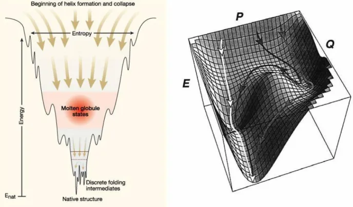
peptide bond isomerization step [7].

Several folding mechanisms have been proposed in the past [104][25][52]. The models all share a pre-folding state followed by a rate-limiting step. The pre-folding state resembles the state of a molten globule [81]. The molten globule has roughly the size of the final folded state and is characterized by the presence of some secondary structural elements.

The transition from the unfolded state to the molten globule is fast, while the transition from the molten globule to the final native conformation is slow and cooperative.

The rate of protein folding lies between 0.1 and 10³seconds, suggesting that protein folding is not a trial-and-error process in which the protein goes through the entire range of possible conformations. In a thought experiment known as the Levinthal’s paradox [65], Levinthal calculated that a 100 residue polypeptide with 10 conformations per residue and 10^-13seconds per conformation would lead to a folding time of 10⁷⁷ years which would exceed the age of the universe. Therefore, protein folding must be a somewhat directed process.

Folding models suggest that the process of folding is not only ruled by thermodynamic considerations but also by kinetic aspects. Mutation studies were able to demonstrate that some amino acid residue exchanges may prevent the protein from completing the folding process without affecting the stability of the already folded state [23].

Thus, one may conclude that the final native conformation does not necessarily have to be the thermodynamically most stable but could simply be the most stable kinetically accessible conformation, so that there may be stable folded conformations for which no folding pathways exist [80].

(34)

Figure 2222....7777:::: Energy Landscape of Protein Energy Landscape of Protein Energy Landscape of Protein Energy Landscape of Protein Folding. Folding. Folding. Folding. Folding funnel showing steps towards completion of native conformation via molten globule states and various folding intermediates (left). Energy landscape displays alternate pathways leading to same native structure at bottom of the funnel (right).

________________________________________________________________

source: http://www.nature.com/horizon/proteinfolding/images/summ_f1.jpg

Protein folding can be visualized by an energy landscape resembling a folding funnel where the most stable conformation is located at the bottom tip of the funnel (Figure 2.7).

The folding process can thus be compared to water moving down the funnel moving towards the final native conformation which could either be the tip of the funnel (global minimum) or one of the humps in between (local minima). This model also shows that the same native conformation may be reached by different kinetic routes. Folding of large proteins with multiple domains contain the additional problem of aggregation and precipitation.

In vitro

, the folding of such large proteins must be carried out at very low protein concentrations.

In

vivo

, protein folding is often assisted by molecular chaperones which temporarily bind to

(35)

unfolded parts of the polypeptide chain to prevent them from aggregation. Other folding- related enzymes include prolyl peptide isomerase and protein disulfide isomerase. Prolyl peptide isomerase accelerates the

cis-trans

isomerization ahead of proline residues [17], while protein disulfide isomerase catalyzes the rearrangement of disulfide bonds after they have been formed [66].

Even though the number of theoretically possible three-dimensional folded protein conformations is astronomical, the actual number of different folds occurring in natural proteins is rather small and estimated to include about 1,000 [43]. This could be explained by the fact that during evolution, tertiary structure has been much more conserved than primary structure. Therefore, proteins which originate from evolutionary related species often have very similar folded conformations despite larger differences in amino acid sequence. The cytochrome and serine protease families represent such examples [82]. In these proteins, large variations in the primary sequence mostly occur at the protein surface while residue changes in the protein core occur in a way that preserves torsion angles.

Residues around the active site of the protein are highly conserved. Homology has not only been observed among different proteins but also within the same polypeptide chain.

Examples for internal homology have been observed for Ferredoxin, parvalbumin, and some immunoglobulins. These proteins usually consist of two or more domains where one domain is thought to have developed from the other by gene duplication [98][70].

2.1.6 2.1.6 2.1.6

2.1.6 Homology Homology Homology Homology

Protein homology is an ambiguous term and can either be understood as evolutionary proximity, similarity in function, similarity in tertiary structure, or sequence identity. Which of the above definitions applies usually depends on the context in which the term is used.

(36)

Generally, two proteins are considered homologous when their sequence is identical above a certain percentage value which depends on the length of the alignment. The degree of sequence identity is determined by the root mean square deviation (rmsd) value which equals to the number of identical residues divided by the length of the shorter protein sequence. For alignments of large proteins, sequence identity of 30% is generally sufficient to assume homology.

It has been shown that sequence identity is highly correlated to structural similarity.

Chotia and Lesk [10] showed that the difference in the structure of two proteins increases as the sequence identity decreases, while Rost [89] demonstrated that for the alignment of long sequences, a sequence identity of 40% and higher guarantees structural similarity. Some proteins have similar folds or similar functions, yet are very low in sequence identity. This includes several mononucleotide-binding domains, also known as Rossman folds [15]

(Chapt. 2.1.4). These domains differ substantially in their primary sequence and have no proven evolutionary relationship, yet still have been found to be similar in three- dimensional structure and function. The question of whether these conformational similarities have arisen from convergent or divergent evolution or happened by pure chance is still open to debate [82]. Examples for functional identity without structural similarity are given by trypsin proteases and serine carboxypeptidases. These enzymes have similar functions but no structural similarities other than their active sites. In this case, functional similarity is thought to have developed from convergent evolution [82].

(37)

2.1.7 2.1.7 2.1.7

2.1.7 Structure Classification Structure Classification Structure Classification Structure Classification

Proteins can be classified by a variety of classification systems. The most widely used systems include SCOP [33], CATH [30], and FSSP [37]:

SCOP (Structural Classification of Proteins) SCOP (Structural Classification of Proteins) SCOP (Structural Classification of Proteins)

SCOP (Structural Classification of Proteins) is a completely manual classification system which orders proteins in a hierarchy using four levels with increasing specificity [33]:

Class:Class:Class:Class: General structural architecture of domains (α-helix, β-sheet, α/β, α+β, multi- domain, membrane proteins, etc.) (Chapt. 2.1.5)

Fold:Fold:Fold:Fold: Similar arrangement of secondary structure with or without evolutionary relationship

Superfamily:Superfamily:Superfamily:Superfamily: Probable common evolutionary relationship with or without sequence similarity

Family:Family:Family:Family: Clear evolutionary relationship either based on sequence identity (30% or greater) or common structure / function.

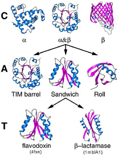
The CATH (Class, Architecture, Topology, Homologous Superfamily)CATH (Class, Architecture, Topology, Homologous Superfamily)CATH (Class, Architecture, Topology, Homologous Superfamily)CATH (Class, Architecture, Topology, Homologous Superfamily) system [30] is built up in a similar manner using four categories (Figure 2.8):

• Class :Class :Class :Class : Total of four classes grouped by general secondary structure content (α-helix, β-sheet, α/β-mixed, few secondary structure)

• Architecture:Architecture:Architecture:Architecture: Total of 35 architectures grouped by similar shapes and structures

• Topology:Topology:Topology:Topology: Similar structure and arrangement of secondary structure without evidence of homology. Comparable to ‘fold’ category in SCOP system (see above)

• Homologous SuperfamilyHomologous SuperfamilyHomologous SuperfamilyHomologous Superfamily: Probable evolutionary relationship without sequence homology (similar to ‘superfamily’ category in SCOP system)

(38)

All levels are assigned automatically according to structure or sequence similarity, except for ‘architecture’ which is assigned manually.

Figure 2222....8888:::: CATH Protein Classification System. CATH Protein Classification System. CATH Protein Classification System. CATH Protein Classification System. First three levels of CATH protein classification system. Levels are ordered in increasing specificity. Class (C) and topology (T) are assigned by automatic methods while architecture (A) is manually assigned.

___________________________

source: http://en.wikipedia.com

(39)

FSSP (Families of Structurally Similar Proteins) FSSP (Families of Structurally Similar Proteins) FSSP (Families of Structurally Similar Proteins)

FSSP (Families of Structurally Similar Proteins) is a fully automated system which is based on the comparison of polypeptide chains rather than protein domains. This system uses the DALI [29] algorithm to classify protein structures by their level of homology. Close homologs (>70% sequence identity) are represented by a single structure while medium homologs (30% - 70% sequence identity) are grouped into structural families [37]. This process results in a reduced subset of representative sequences which can be used for searching remote homologous proteins. The FSSP system has the advantage of providing immediate access to structural alignments. In addition, it reports the degree of sequence identity based on root-mean-square deviation (Chapt. 2.1.6). The disadvantage of this system is that it may produce misleading results especially with regard to multi-domain proteins, since important pieces of information on structural domains are neglected.

2.1.8 2.1.8 2.1.8

2.1.8 Structure Determination Methods Structure Determination Methods Structure Determination Methods Structure Determination Methods

X-ray crystallography is the most widely used method for analyzing protein structures. More than 85 % of structures stored in the Protein Data Bank (PDB) have been determined by x-ray diffraction techniques [45]. In order for a protein to be measured by this method, a large and well ordered protein crystal needs to be grown. Building protein crystals is a slow, tedious and not always successful process. Crystals are grown in supersaturated solutions by slowly decreasing the solubility of the protein while empirically varying a number of external parameters such as temperature, pH, and the concentration of additives, in an attempt to find optimal conditions for crystal growth. Crystals may then develop in a setup such as a hanging drop after an initial nucleation step and usually remain high in solvent content after crystallization (on average between 40-60%). Thus, the three-

(40)

θ λ 2d sin n =

dimensional structure of crystallized proteins has a high resemblance to the native structure in solution.

A protein crystal suitable for measurement contains about 10¹⁵ molecules. During measurement, the crystal is irradiated with x-rays while the two-dimensional diffraction patterns representing ‘slices’ of the crystal are being recorded on photographic film or a charged coupled device (CCD) image sensor [32]. While the crystal is rotated in small steps around slightly more than 180° (Ewald Sphere), diffraction patterns are recorded from all angles of the crystal. A diffraction pattern contains multiple reflections where each reflection has a specific intensity and position recorded in Miller indices (

h,k,l

). Miller indices are lattice coordinates which represent points the original crystal lattice in reciprocal space. The inverse relationship between crystal lattice and diffraction pattern coordinates is reflected in Bragg’s Law of diffraction [6]:

In the above equation, λ is the x-ray wavelength, while d stands for the distance in lattice points of the crystal lattice in real space, and θ is the reflection angle. Braggs Law shows that an interference pattern based on constructive interference of the scattered waves occurs whenever the phase shift is a multiple of 2π.

The final goal of x-ray diffraction analysis is the construction of an electron density map which displays the position of each atom in a protein crystal. Electron densities of each position in real space ρ(x,y,z) are calculated by summation of the intensity and positional information on all the recorded diffraction patterns using a method known as Fourier synthesis or Fourier transform: